University of Groningen
Comparing Generative Adversarial Network Techniques for Image Creation and Modification
Pieters, Mathijs; Wiering, Marco
Published in: ArXiv
IMPORTANT NOTE: You are advised to consult the publisher's version (publisher's PDF) if you wish to cite from it. Please check the document version below.
Document Version
Early version, also known as pre-print
Publication date: 2018
Link to publication in University of Groningen/UMCG research database
Citation for published version (APA):
Pieters, M., & Wiering, M. (2018). Comparing Generative Adversarial Network Techniques for Image Creation and Modification. ArXiv.
Copyright
Other than for strictly personal use, it is not permitted to download or to forward/distribute the text or part of it without the consent of the author(s) and/or copyright holder(s), unless the work is under an open content license (like Creative Commons).
Take-down policy
If you believe that this document breaches copyright please contact us providing details, and we will remove access to the work immediately and investigate your claim.
Downloaded from the University of Groningen/UMCG research database (Pure): http://www.rug.nl/research/portal. For technical reasons the number of authors shown on this cover page is limited to 10 maximum.
Comparing Generative Adversarial Network
Techniques for Image Creation and Modification
Mathijs Pieters
Institute of Artificial Intelligence University of Groningen, The Netherlands
Marco Wiering
Institute of Artificial Intelligence University of Groningen, The Netherlands
Abstract
Generative adversarial networks (GANs) have demonstrated to be successful at generating realistic real-world images. In this paper we compare various GAN techniques, both supervised and unsupervised. The effects on training stability of different objective functions are compared. We add an encoder to the network, making it possible to encode images to the latent space of the GAN. The gener-ator, discriminator and encoder are parameterized by deep convolutional neural networks. For the discriminator network we experimented with using the novel Capsule Network, a state-of-the-art technique for detecting global features in im-ages. Experiments are performed using a digit and face dataset, with various visualizations illustrating the results. The results show that using the encoder network it is possible to reconstruct images. With the conditional GAN we can alter visual attributes of generated or encoded images. The experiments with the Capsule Network as discriminator result in generated images of a lower quality, compared to a standard convolutional neural network.
1
Introduction
Generative Adversarial Networks (GANs) [Goodfellow et al., 2014] are a subclass of generative models that have received a lot of attention because of their ability to generate realistic high quality images. The GAN setup consists of two networks, a generator and discriminator, that compete against each other in a two-player minimax game. An analogy for this minimax game using the production of money is as follows. The generator is a counterfeiter that aims to create realistic money, whereas the discriminator’s aim is to differentiate money created by the generator from real money. Both systems are trained simultaneously, and the competition should improve the systems until the generator produces counterfeits that are indistinguishable from real money. The generator does not have access to the real data, it only learns from the feedback from the discriminator.
More recently, people started to apply the GAN framework to other problems, such as text generation and image-to-image translation [Zhang et al., 2017, Isola et al., 2016]. Since the introduction of the GAN, many variants have been proposed. A lot of research has been devoted to finding GAN algorithms that are more stable [Arjovsky et al., 2017, Gulrajani et al., 2017, Berthelot et al., 2017]. Although many papers claim to have found a significant improvement, Lucic et al. [2017] show that there is no evidence to support these claims.
In this research we provide an overview of various GAN techniques. We compare standard GANs [Goodfellow et al., 2014] with conditional GANs [Mirza and Osindero, 2014], and supervised networks with unsupervised networks [Chen et al., 2016]. Furthermore, we use an encoder making it possible to generate images that resemble specific images. This approach is very similar to the encoder network in a variational autoencoder [Kingma and Welling, 2013]. Finally, we compare a deep convolutional neural network with the novel Capsule Network as parameterization of the discriminator. These comparisons are performed on two datasets. The first dataset is MNIST [LeCun
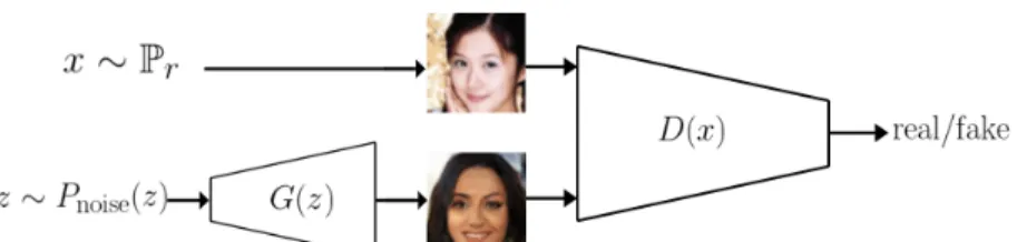
Figure 1: Graphical representation of a GAN.
et al., 1998], a dataset with images of handwritten digits. The second dataset we used is CelebA [Liu et al., 2015], containing images of faces.
We explain the used methods in section 2, followed by section 3 where we explain the experimental setup and show the results. Finally, in section 4 we draw a conclusion and propose future research.
2
Methods
2.1 Generative Adversarial Networks
A Generative Adversarial Network consists of two competing networks, the generator and the
discriminator. The generator tries to learn a mapping from a noise distribution to the real data distributionPr, while the discriminator’s task is to distinguish real data samples from samples
generated by the generatorPg. The flow of data in a GAN is illustrated in Figure 1. Formally, the
generatorGtransforms a noise samplezinto a samplexˆ=G(z)(wherez ∼Pnoise(z)is sampled
from a certain noise distribution such as a uniform distribution). This noise samplezis also referred to as the latent vector. The discriminator, indicated byD(x), learns the probability thatxoriginates from the real data distribution, rather than fromPg.Dis trained such that it maximizes the probability
of classifying the samples fromPr as real, and the samples fromPgas fake. At the same time,
Gis trained to minimizelog(1−D(xˆ)). The lower this value, the higherD(xˆ), indicating a high probability thatxˆis considered to be generated by the real data distribution. The training of the generatorGand the discriminatorDis defined as the following minimax game:
min
G maxD Ex∼Pr[logD(x)] +Ex∼ˆ Pg[log(1−D(xˆ))] (1)
We refer to this value function asV(D, G). The loss function for the discriminator and generator are respectively defined as:
LGAN
D =−Ex∼Pr[logD(x)]−Ex∼ˆ Pg[log(1−D(xˆ))] (2)
LGAN
G =Ex∼Pˆ g[log(1−D(xˆ))] (3)
In practice we trainGto maximizelog(D(xˆ)), because at the start of training the generated samples
ˆ
xare of poor quality, making it easy for the discriminator to distinguishPgfromPr. This could
saturatelog(1−D(xˆ)). Both the generator and the discriminator must be differentiable functions. In section 3 we will go into more depth regarding the used networks that representGandD.
2.2 Conditional GAN
We can extend the standard GAN such that we can generate samples conditioned on some variable [Mirza and Osindero, 2014]. This can be very helpful when we want to generate samples of a specific mode. This setup is referred to as conditional GAN, and works as follows. We include an additional variableyin the model, such that we generate and discriminate samples conditioned ony. The goal for the generator is then to generate samplesxˆthat are both realistic and match the contexty. It is possible to use various types of data fory, such as discrete labels [Mirza and Osindero, 2014], text [Reed et al., 2016] or even images [Isola et al., 2016]. One of the benefits of a conditional GAN is that it is able to learn improved representations for multi-modal data. The objective function for a conditional GAN is:
min
where Py is the conditional density distribution. In the conditional GAN, we concatenate the
conditional variabley to the input of every layer, for both the generator and discriminator. A conditional GAN is a supervised network that needs for each data pointxa labely. This network has many similarities with InfoGAN [Chen et al., 2016], an unsupervised conditional GAN, which we will introduce in the next section.
2.3 InfoGAN
In the standard GAN setup (as described in section 2.1), there is no reason to expect that individual dimensions of the latent vector correspond to specific semantic features in the generated data. Preliminary research has shown that varying a single dimension of the latent vector has very little influence on the generated images. In section 2.2 we discussed a supervised method to train a GAN, where we ideally can change visual features of the generated data, by changing the conditional variabley. However, in many cases we have sparse labels, or no labels at all for the given dataset. Chen et al. [2016] proposed to use an additional latent codec, that is used together withz as an input for the generator. In contrast to the conditional GAN, the discriminator does not know about
c(oryin the case of the conditional GAN). Because the discriminator has no information about
c, the easiest solution for the generator would be to ignoreccompletely. In order to prevent this, Chen et al. [2016] proposed to add an additional term to the loss functions that promotes high mutual information betweencandG(z,c). Mutual information betweenXandY is denoted asI(X;Y), and measures the reduction of uncertainty inY whenXis observed, and vice versa. The minimax game we try to solve in InfoGAN is then the same as Equation 1, with−I(c;G(z,c))added. The posteriorP(c|ˆx), needed to determineI(c;G(z,c)), is intractable to calculate. Therefore we make use of an additional distributionQ(c|ˆx)that approximatesP(c|ˆx). Chen et al. [2016] show that you can maximize the following lower bound in order to maximizeI(c;G(z,c)):
I(c;G(z,c))≥Ec∼P(c),x∼ˆ G(z,c)[logQ(c|ˆx)] (5)
We refer to this lower bound asLI(G, Q), whereQis a neural network that shares all layers withD
(except the last one). The last layer ofQgives as an output the conditional distributionQ(c|ˆx). The minimax game for InfoGAN is as follows:
min
G,QmaxD VInfoGAN(D, G, Q) =V(D, G)−λILI(G, Q) (6)
whereλIis a hyperparameter. The latent variableccan consist of multiple separate distributions.
In this research we focus on categorical and continuous latent codes. The first is represented by a softmax nonlinearity inQ, the latter is represented by a factored Gaussian. In section 3 we will provide the used latent codes per dataset.
2.4 Wasserstein GAN
GANs are known to be very difficult to train for various reasons [Arjovsky and Bottou, 2017]. With the original value function as defined in 1, a strong discriminator can cause vanishing gradients. With the improved value function, where the generator maximizeslog(D( ˆx)), the training updates can be very unstable. In both situations the generator may not converge to a stable network that produces realistic samples. In the work of Arjovsky et al. [2017] an alternative value function named Wasserstein GAN (WGAN) is proposed. The authors show that the value function of WGAN has better convergence properties compared to the standard value function. WGAN makes use of the Wasserstein distanceW(q, p), which intuitively can be interpreted as the minimum cost of moving mass such that distributionqis transformed to distributionp(where cost is the transformed mass multiplied with the distance it has been moved). The WGAN value function is as follows:
min
G maxD∈DEx∼Pr[D(x)]−Ex∼ˆ Pg[D(xˆ)] (7)
whereDis the set of functions that are 1-Lipschitz1. Because the discriminator in the WGAN does not
discriminate anything (e.g. real images from fake images), it is referred to ascritic. With an optimal critic, the generator minimizesW(Pr,Pg)when we minimize the value function from Equation 7.
In order to enforce the Lipschitz constraint, Arjovsky et al. [2017] make use of clipping the weights of the critic between[−c, c]for some positive constantc. However, Gulrajani et al. [2017] show that
1
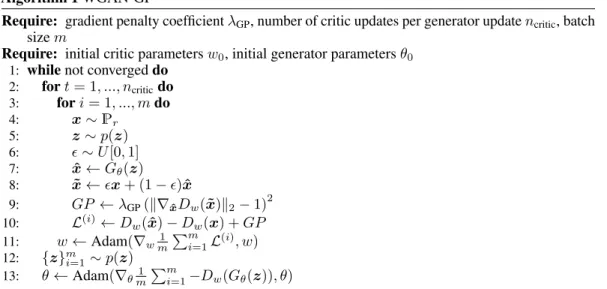
Algorithm 1WGAN-GP
Require: gradient penalty coefficientλGP, number of critic updates per generator updatencritic, batch
sizem
Require: initial critic parametersw0, initial generator parametersθ0
1: whilenot convergeddo
2: fort= 1, ..., ncriticdo 3: fori= 1, ..., mdo 4: x∼Pr 5: z∼p(z) 6: ∼U[0,1] 7: xˆ←Gθ(z) 8: x˜←x+ (1−)xˆ 9: GP ←λGP(k∇xˆDw(x˜)k2−1) 2 10: L(i)←D w(xˆ)−Dw(x) +GP 11: w←Adam(∇wm1 Pm i=1L (i), w) 12: {z}m i=1∼p(z) 13: θ←Adam(∇θm1 P m i=1−Dw(Gθ(z)), θ)
weight clipping can result in undesired behaviour such as exploding or vanishing gradients. Gulrajani et al. [2017] propose to use a gradient penalty to enforce the Lipschitz constraint, this method is referred to as WGAN with gradient penalty (WGAN-GP). The gradient penalty is defined as
Ex∼P˜ ˜x[(k∇x˜D(x˜)k2−1)
2] (8)
whereP˜xis the distribution sampled uniformly along straight lines between points in the distributions
PrandPg(see line 8 in Algorithm 1). Because the gradient penalty is determined for each sample
independently (see Algorithm 1), we omit batch normalization in the critic. Batch normalization would namely create dependence between the samples within a batch. We should train the critic till optimality, but in practice we train the critic for a specific amount of iterations indicated byncritic.
The coefficientλGP, shown on line 9 in Algorithm 1, is used to make sure the effect of the gradient
penalty is significant.
2.5 Encoder
In the standard GAN setup we can create random samples that seem to originate from the real data distributionPr. However, we can not create samples that look similar to some specific data points in
Pr. Formally, we would like to have a method such that we can find a latent vectorzˆfor a samplex,
such thatG(zˆ)≈x(as illustrated in Figure 2). This method has many similarities with a variational autoencoder [Kingma and Welling, 2013], where the decoder is replaced by the generator. In order to find such a latent vector, we will use an encoderEthat has as objectiveG(E(x))≈xfor all
x∼Pr. In order to train the encoder we can make use of several loss functions [Zhao et al., 2017].
In this research we focused on minimizing the following loss function:
LE=Ex∼Pr[ 1 N X p∈P |G(E(x))(p)−x(p)|]
whereNis the number of pixels,pis the index of a pixel, andPis the set of indices of all pixels. Note that when using either the condition GAN or infoGAN, we need to encode an additional variable (yorcrespectively). Similar to the generator and discriminator, the encoder is parameterized by a neural network.
2.6 Capsule Network
In the original paper that introduced GANs [Goodfellow et al., 2014] the authors use a multilayer perceptron for both the generator and discriminator. Although this network performs reasonably well on a simple dataset (e.g. MNIST), on more complex datasets the results are not good. Convolutional neural networks (CNNs) are widely used for supervised learning in computer vision problems. In more recent work [Radford et al., 2015] the GAN setup was succesfully combined with a CNN (DCGAN) to create state of the art results. Radford et al. [2015] proposed several improvements such as using strided convolutions, batch normalization [Ioffe and Szegedy, 2015], and the ReLU activation function. Although CNNs are good at detecting local features, the technique is less effective at detecting (spatial) relationships between these different features. Part of this problem is caused by the invariant detection of features, CNNs process the likelihood of features without subsequently processing the properties of these features (e.g. angle or size). Sabour et al. [2017] propose a network that uses capsules to present an object or features of an object. The activity of these capsules is represented by a vector, where the length of the vector represents the likelihood of an object or part of an object. The orientation of the vector represents the specific properties of this object. When using multiple layers of capsules, the predictions of higher-level capsules are determined by the lower-level capsules and a transformation matrix. Because lower-level capsules also capture the instantiation of parts of an object, high-level capsules can make better predictions about the global features of an object.
We will now describe the capsule network formally. Letsjdenote the input vector of capsulej, then
the output vector is defined as
vj=squash(sj) = ksjk2 1 +ksjk2 sj ksjk (9) Note that the orientation of the vector is preserved, while short vectors are reduced to almost zero length, and long vectors are reduced to approximately unit length. For a capsulejthe total input is a weighted sum of all the vectorsuˆj|i, whereuˆj|iis a prediction vector of capsulei(in the layer
below) connected to capsulej, calculated as
ˆ
uj|i=Wijvi (10)
whereWijis a weight matrix andvithe output of a capsule in the layer below. The total input for
capsulejis then calculated as follows
sj =
X
i
cijuˆj|i (11)
wherecij are coupling coefficients. The coupling coefficients are determined by a technique called
"routing-by-agreement" [Sabour et al., 2017], such that the coefficients are increased when the prediction vector is similar to the output of a parent capsule, and decreased when they are dissimilar. Similarity between two vectors is measured as the scalar product of these two vectors. The coupling coefficients of capsulejand all the parent capsules sum to 1, enforced by
cij =
exp(bij)
P
kexp(bik)
(12) wherebij are the log prior probabilities that capsulesiandjshould be connected. The coupling
coefficients are refined multiple times to make connections between agreeing capsules stronger, as described in Algorithm 2.
3
Experiments
In our experiments we make use of two datasets, MNIST [LeCun et al., 1998] and CelebA [Liu et al., 2015]. The discussed techniques are very general, making them applicable to a broad range of image datasets. We use two datasets to compare the techniques on relatively simple, and more complex images.
First of all, we want to generate realistic looking images. We will compare the generated images when different discriminators are used during training. By means of the conditional GAN we will experiment with generating images with certain specified attributes. Using the encoder network, we aim to perfectly reconstruct the images from the dataset. Finally, by combining a conditional GAN with the encoder network, we will experiment with changing visual attributes of reconstructed images.
Algorithm 2Dynamic Routing
Require: prediction vectorsuˆj|i, routing iterationsr, capsule layerl
Require: bijinitial routing logits for all capsulesiin layerland capsulesjin layer(l+ 1)
1: forriterationsdo
2: forall capsulesiin layerldo
3: ci←softmax(bi) .Eq. 12
4: forall capsulesiin layerl+ 1do
5: sj ←Picijuˆj|i
6: forall capsulesjin layerl+ 1do
7: vj←squash(sj) .Eq. 9
8: forall capsulesiin layerldo
9: forall capsulesjin layerl+ 1do
10: bij←bij+uˆj|i·vj
3.1 MNIST
The first dataset we used is MNIST [LeCun et al., 1998], consisting of 60,000 1-channel images of handwritten digits with a size of28×28pixels. For supervised learning (conditional GAN), we can make use of the image labels indicating the digit.
3.2 CelebA face images
The second dataset we used to compare the techniques is CelebA [Liu et al., 2015]. This dataset consists of 202,599 images of faces, every image is labelled with 40 binary attributes. Examples of these attributes are smiling, wearing hat, mustache, and blond hair. The images are rescaled and cropped to images of64×64pixels. The original size of the images is178×218pixels.
3.3 Architectures
We will now discuss the architectures used in this research. The generator and discriminator are similar to the convolutional neural networks proposed by Radford et al. [2015]. As described in Table 1 we use the same encoder for both datasets. For the generator we found that the results are best if we use different networks for the different datasets. In the generator we use transposed convolutional layers with stride 2, in order to upscale the images. In all experiments we used the Adam optimizer [Kingma and Ba, 2014] to minimize the loss functions, with a learning rate of10−4and batch size of
64. For the Adam optimizer we used 0.5 forβ1and0.9forβ2when training WGAN-GP, otherwise
we used 0.5 and 0.99 respectively. For WGAN-GP we used a gradient penalty coefficient of 10 and 5 critic updates per generator update, similar to Arjovsky et al. [2017]. These parameters are indicated in Algorithm 1 byλGPandncritic, respectively. We trained all models for 60 epochs. In all
experiments with the MNIST dataset we used azvector of dimension 64, whereas with the CelebA dataset we used vectors of dimension 128. In all experiments the latent vector follows the uniform distributionU(−1,1). When training infoGAN the additionalQnetwork shares all layers (except the last one) with the discriminator. The final output for the conditional distributionQ(c|ˆx)is determined by using two fully-connected layers, of which the first one has 128 hidden nodes. The second layer has an output dimension that matches the predetermined dimension of the latent codez. When we train a conditional GAN or infoGAN, the output dimension of networkEis equivalent to the total dimensions of the latent vector and vectorsyorc. Note that in this context the latent vectorzis not really a noise vector.
In the experiments with the capsule network as discriminator we used the following parameters. The network is similar to the one proposed by Sabour et al. [2017], with the only differences that the first layer has 128 filters instead of 256, and that the final layer consists of only a single capsule instead of 10 capsules. Our network has a single output capsule because the task is binary classification (differentiate real from generated images), whereas Sabour et al. [2017] used 10 output capsules because they tried to classify digits in the MNIST dataset. The first layer is a standard convolutional layer with 128 convolutional filters with size9×9, a stride of 1, and the ReLU activation function. In the second layer we use a convolutional capsule layer with 32 channels, where each channel is an 8 dimensional capsule. This 8 dimensional capsule has filters of size9×9and a stride of 2. Using
dynamic routing (as described in Algorithm 2), we map the output of the second layer to the third and also final layer. For the dynamic routing algorithm we use 3 routing iterations. The final layer consists of a single 16 dimensional capsule. Sabour et al. [2017] use an additional reconstruction loss to promote regularization, but in our experiments we omitted this term.
Table 1: Architectures for the encoder, generator and discriminator. FC stands for a fully-connected layer, BN denotes batch normalization, and t-conv is short for transposed convolution.z-dim is 64 when using MNIST, for CelebA it is 128. All the convolutional filters are of size5×5, with stride 2. Note that we use different generator networks for the two datasets. lRelU is short for leaky ReLU, for this activation function we used a slope coefficient of 0.2.
Encoder Generator MNIST Generator CelebA Discriminator 64 conv. lReLU 7×7×128 FC, BN, ReLU 4×4×512 FC, BN, ReLU 64 conv. lReLU 128 conv. BN, lReLU 128 t-conv. BN, ReLU 256 t-conv. BN, ReLU 128 conv. BN, lReLU 256 conv. BN, lReLU 1 t-conv. tanh 128 t-conv. BN, ReLU 256 conv. BN, lReLU 512 conv. BN, lReLU 64 t-conv. BN, ReLU 512 conv. BN, lReLU
z-dim FC, tanh 3 t-conv. tanh 1 FC, sigmoid
3.4 Results
The shown results are from the first experiments after hyperparameter tuning. We ran multiple experiments to make sure the result are similar in different runs, ensuring that the results are representative.
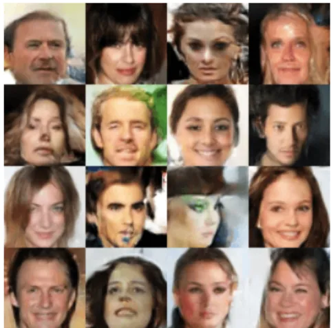
We found that using the WGAN-GP training, the results are of higher quality compared to the standard GAN training objective. In Figures 3 and 4 you can see generated samples for the two datasets, using the network as described in Table 1, trained with WGAN-GP.
Figure 3: Generated samples for the MNIST dataset. The used networks are described in Table 1, trained with WGAN-GP.
Figure 4: Generated samples for the CelebA dataset. The used networks are described in Table 1, trained with WGAN-GP.
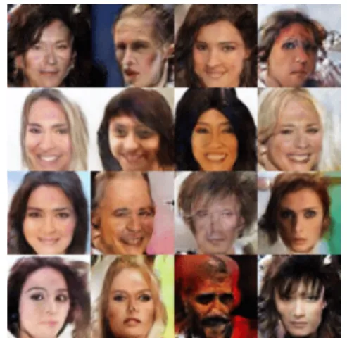
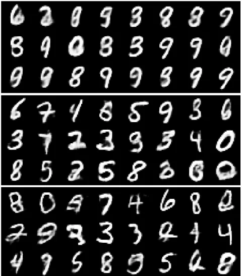
In Figures 5 and 6 the results of using the capsule network as a discriminator are shown. For the training of this network we used the standard GAN objective (Equation 1). We did not manage to combine the capsule network with the WGAN-GP objective, because determining the gradient penalty (Equation 8) is nontrivial when using dynamic routing (Algorithm 2). Figures 7 and 8 show the results of using standard convolutional network (as described in Table 1) with the standard GAN objective. The generated samples using the capsule network are of a lower quality compared to the samples generated when using a standard convolutional network as discriminator.
Figure 5: Generated samples for the MNIST dataset, trained using the cap-sule network as discriminator. The gen-erator is described in Table 1.
Figure 6: Generated samples for the CelebA dataset, trained using the cap-sule network as discriminator. The gen-erator is described in Table 1.
Figure 7: Generated samples for the MNIST dataset. The used networks are described in Table 1, trained using the standard GAN objective.
Figure 8: Generated samples for the CelebA dataset. The used networks are described in Table 1, trained using the standard GAN objective.
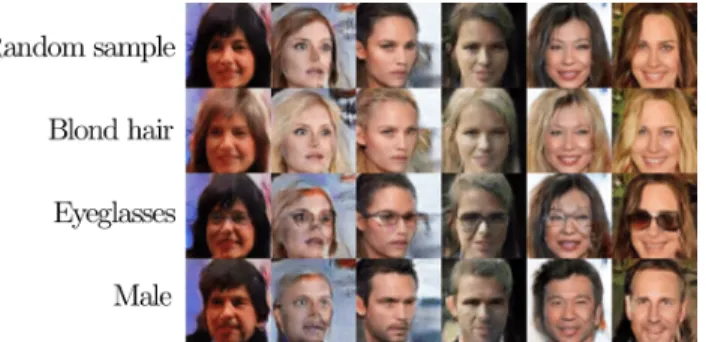
For the conditional GAN we performed the following experiments. When training the conditional GAN we could use either the standard GAN objective or the WGAN-GP objective. We found that, similar to the unconditional GAN, the results are better when using WGAN-GP. In Figure 9 the results for the MNIST dataset are shown. For the conditional variable we used the digit classes. The results show that this supervised network makes it possible to generate images of distinct classes, where the style of these images is determined by the latent noise vector. The results of the conditional GAN for the CelebA dataset are shown in Figure 10, where we made use of the binary attributes blond hair, eyeglasses, and male. The results show that by varying the conditional variables, we can visually change the sample generated from the same noise vector. Figures 22 and 23 show more results for the conditional GAN using the CelebA dataset.
Figure 9: Random samples for MNIST, conditioned on digit label. Every column corresponds to a unique label, the samples in a row have the same latent noise vector. The used networks are described in Table 1, trained with the conditional WGAN-GP.
Figure 10: Random samples for CelebA, conditioned on three different attributes. Every column corresponds to a unique latent noise vector. The used networks are described in Table 1, trained with the conditional WGAN-GP.
In order to generate images that look similar to a specific image we made use of the encoder network. Figures 11 and 12 show the results of the encoding and reconstruction for MNIST and CelebA, respectively. For MNIST we find that the encoding results in very similar pictures. In many images it is difficult to distinguish the real images from their encoded and reconstructed counterparts. The encoding of the CelebA images shows that high frequency details are lost. However, the encoded images still show a great similarity with the original images.
Figure 11: Image encoding and reconstruction for the MNIST dataset. Rows 1, 3, and 5 are the original images taken from MNIST, rows 2, 4, and 6 are the corresponding reconstructed images based on the encoding. The used networks are described in Table 1, trained with WGAN-GP.
Figure 12: Image encoding and reconstruction for the CelebA dataset. Rows 1, 3, and 5 are the original images taken from CelebA, rows 2, 4, and 6 are the corresponding reconstructed images based on the encoding. The used networks are described in Table 1, trained with WGAN-GP.
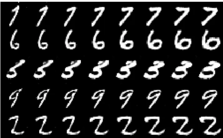
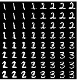
We will now compare some results for the infoGAN setup. For the MNIST dataset we experimented with using a categorical variable with 10 classes, in the hope that every class corresponds to a unique digit. Additionally, we used a continuous variable following a uniform distribution. The results for this experiment are illustrated in Figures 13 and 14, respectively. By varying the categorical variable, we observe a change in digit class. However, we see that for digits that look similar (e.g. 5 and 9), a single categorical class can contain both digit classes. Varying the continuous latent variable influences the width of the generated digits. In Figure 15 the results are shown for varying a continuous latent variable on the CelebA dataset. We observe that this variable has an influence on hair colour, changing the colour from dark to bright.
Figure 13: Manipulation of categorical latent variablecfor MNIST samples. Every column corre-sponds to a unique category, every row has a fixed latent vector. The used networks are described in Table 1, trained with InfoGAN.
Figure 14: Manipulation of continuous latent variablecfor MNIST samples. Every row corresponds to a unique latent variable, where we varycbetween -1 and 1. The used networks are described in Table 1, trained with InfoGAN.
Figure 15: Manipulation of continuous latent variablecfor CelebA samples. The variable is varied between -1 and 1, every row has a unique latent vector. The used networks are described in Table 1, trained with InfoGAN.
4
Conclusion and Future Research
In this paper we compared several GAN techniques for image creation and modification. We found that the standard GAN can be unstable, using WGAN-GP results in more stable training and the generated images are of a higher quality. With the standard GAN, we often observed a mode collapse. The mode collapse usually occurred after many epochs, making training very ineffective. It can take a lot of hyperparameter tuning to find the correct balance between the generator and discriminator, making sure one doesn’t outperform the other. When using WGAN-GP, this balance is less of a concern because the critic is trained till optimality.
We compared two conditional GANs, namely the standard conditional GAN that is supervised and InfoGAN, an unsupervised network. The supervised conditional GAN makes it possible to vary spe-cific visual attributes within an image, given that the dataset contains labels for these attributes. With infoGAN, it is also possible to change visual attributes of the generated images. However, in contrast to the supervised conditional GAN, it is not possible to specify which visual attributes we would like to change. Depending on the dataset and the chosen latent distribution, the network learns a disentan-gled representation. We also used an encoder network that makes it possible to create a reconstruction of an image, independent of the used GAN variant. The reconstructions for MNIST are seemingly perfect, whereas for the CelebA dataset the reconstructions are good but blurry. Using this technique we can apply dimensionality reduction, similar to a variational autoencoder [Kingma and Welling, 2013]. We experimented with using the novel capsule network as discriminator. This however did not lead to satisfying results. We expect that this is due to the relatively small and shallow network.
Because of the rapid development of GAN techniques, many opportunities for future research are remaining. In follow-up research we would like to experiment with reconstructing images using gradient based approaches to generate latent vectors, similar to Lipton and Tripathi [2017] their approach. Furthermore, more experiments with different loss functions for the encoder network are needed. We could even extend this, using the discriminator in a GAN as a measure for the reconstruction objective, as introduced by Larsen et al. [2016]. More experiments with methods that improve the stability of GANs are needed, such as spectral normalization [Takeru Miyato, 2018] and using two discriminators [Nguyen et al., 2017]. Finally, we want to test the discussed methods on different and more complex datasets.
5
Acknowledgements
We would like to thank the Center for Information Technology of the University of Groningen for their support and for providing access to the Peregrine high performance computing cluster.
References
Martin Arjovsky and Léon Bottou. Towards principled methods for training generative adversarial networks. arXiv preprint arXiv:1701.04862, 2017.
Martin Arjovsky, Soumith Chintala, and Léon Bottou. Wasserstein GAN. arXiv preprint arXiv:1701.07875, 2017.
David Berthelot, Tom Schumm, and Luke Metz. BEGAN: Boundary equilibrium generative adver-sarial networks. arXiv preprint arXiv:1703.10717, 2017.
Xi Chen, Yan Duan, Rein Houthooft, John Schulman, Ilya Sutskever, and Pieter Abbeel. InfoGAN: Interpretable representation learning by information maximizing generative adversarial nets. In
Advances in Neural Information Processing Systems, pages 2172–2180, 2016.
Ian Goodfellow, Jean Pouget-Abadie, Mehdi Mirza, Bing Xu, David Warde-Farley, Sherjil Ozair, Aaron Courville, and Yoshua Bengio. Generative adversarial nets. InAdvances in neural informa-tion processing systems, pages 2672–2680, 2014.
Ishaan Gulrajani, Faruk Ahmed, Martin Arjovsky, Vincent Dumoulin, and Aaron Courville. Improved training of Wasserstein GANs. arXiv preprint arXiv:1704.00028, 2017.
Sergey Ioffe and Christian Szegedy. Batch normalization: Accelerating deep network training by reducing internal covariate shift.CoRR, abs/1502.03167, 2015.
Phillip Isola, Jun-Yan Zhu, Tinghui Zhou, and Alexei A Efros. Image-to-image translation with conditional adversarial networks. arXiv preprint arXiv:1611.07004, 2016.
Diederik P. Kingma and Jimmy Ba. Adam: A method for stochastic optimization. CoRR, abs/1412.6980, 2014.
Diederik P Kingma and Max Welling. Auto-encoding variational bayes. arXiv preprint arXiv:1312.6114, 2013.
Anders Boesen Lindbo Larsen, Søren Kaae Sønderby, Hugo Larochelle, and Ole Winther. Autoencod-ing beyond pixels usAutoencod-ing a learned similarity metric. In33rd International Conference on Machine Learning (ICML 2016) International Conference on Machine Learning, 2016.
Yann LeCun, Léon Bottou, Yoshua Bengio, and Patrick Haffner. Gradient-based learning applied to document recognition. Proceedings of the IEEE, 86(11):2278–2324, 1998.
Zachary C Lipton and Subarna Tripathi. Precise recovery of latent vectors from generative adversarial networks. arXiv preprint arXiv:1702.04782, 2017.
Ziwei Liu, Ping Luo, Xiaogang Wang, and Xiaoou Tang. Deep learning face attributes in the wild. In
Mario Lucic, Karol Kurach, Marcin Michalski, Sylvain Gelly, and Olivier Bousquet. Are GANs created equal? a large-scale study. arXiv preprint arXiv:1711.10337, 2017.
Mehdi Mirza and Simon Osindero. Conditional generative adversarial nets. arXiv preprint arXiv:1411.1784, 2014.
Tu Nguyen, Trung Le, Hung Vu, and Dinh Phung. Dual discriminator generative adversarial nets. In
Advances in Neural Information Processing Systems, pages 2667–2677, 2017.
Alec Radford, Luke Metz, and Soumith Chintala. Unsupervised representation learning with deep convolutional generative adversarial networks.CoRR, abs/1511.06434, 2015.
Scott E. Reed, Zeynep Akata, Xinchen Yan, Lajanugen Logeswaran, Bernt Schiele, and Honglak Lee. Generative adversarial text to image synthesis.CoRR, abs/1605.05396, 2016.
Sara Sabour, Nicholas Frosst, and Geoffrey E Hinton. Dynamic routing between capsules. In
Advances in Neural Information Processing Systems, pages 3859–3869, 2017.
Masanori Koyama Yuichi Yoshida Takeru Miyato, Toshiki Kataoka. Spectral normalization for generative adversarial networks.International Conference on Learning Representations, 2018. Yizhe Zhang, Zhe Gan, Kai Fan, Zhi Chen, Ricardo Henao, Dinghan Shen, and Lawrence Carin.
Adversarial feature matching for text generation.arXiv preprint arXiv:1706.03850, 2017. Hang Zhao, Orazio Gallo, Iuri Frosio, and Jan Kautz. Loss functions for image restoration with
A
Appendix
A.1 Bilinear Interpolation on Latent Space
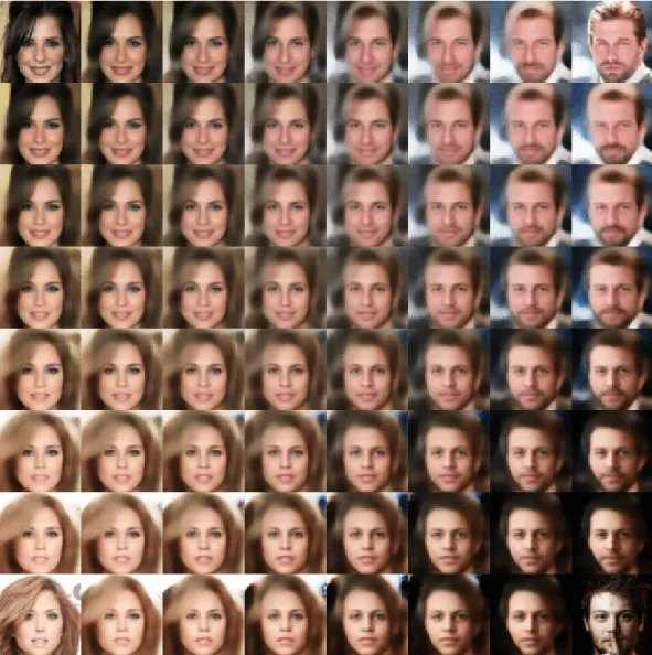
In order to show the process of encoding images as well as applying interpolation between images we use the following process. Every corner of a figure contains a real image from the given dataset. We use the encoder network to generate four latent vectors for the given images, and subsequently apply bilinear interpolation between these four vectors. These vectors are then used as an input for the generator, producing the final images. An example for bilinear interpolation on the MNIST dataset is given in Figure 16, examples for the CelebA dataset are shown in Figures 18 and 19. In Figure 20 we show bilinear interpolation of four random latent space samples, using the CelebA dataset with images of size 128×128.
Figure 16: Bilinear interpolation on the latent space for encoded MNIST samples. The used networks are described in Table 1, trained with WGAN-GP.
A.2 Sample Diversity
During training we samplezfrom a uniform distributionU(−1,1). However, we found that the generated images depend on the sampled distribution. Figures 17 and 21 show the results of sampling the latent vector from different distributions (note that the networks are still trained onz∼ U(−1,1)). We observe that when we sample from a distribution with a smaller range, the samples are of a higher quality but are less diverse. ConsideringU(−r, r), we can in general tradeoff diversity for quality. The higherr, the more diversity in the samples and the lower the quality.
A.3 Conditional Attributes
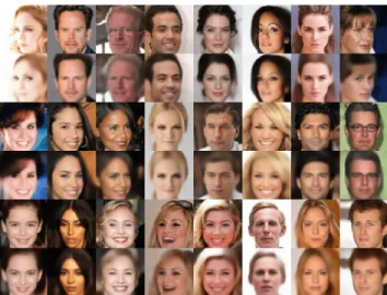
By combining the encoder network with a conditional GAN, it is in theory possible to change visual attributes of a specific image. In Figure 22 we demonstrate this. We start with encoding and reconstructing the original random samples. In order to change the visual attributes, we change the conditional variableyof the corresponding attribute. We feed this adapted conditional variable together with the encoded latent vector into the generator, producing the images in the bottom rows. Figure 23 shows that it is also possible to use multiple binary attributes at once.
Figure 17: Random generated samples for the MNIST dataset. Latent vectors of the top three rows are sampled fromU(−0.2,0.2), the three middle rows fromU(−0.5,0.5), and the bottom rows from
Figure 18: Bilinear interpolation on latent space for encoded CelebA samples. The used networks are described in Table 1, trained with WGAN-GP.
Figure 19: Bilinear interpolation on latent space for encoded CelebA samples. The used networks are described in Table 1, trained with WGAN-GP.
Figure 20: Bilinear interpolation on latent space for random noise vectors. Dataset used is CelebA with images of size 128×128. The used networks are described in Table 1, trained with WGAN-GP.
Figure 21: Random generated samples of size 128×128 for the CelebA dataset. Latent vectors of top three rows are sampled fromU(−0.2,0.2), the three middle rows fromU(−0.5,0.5), and the bottom rows fromU(−0.8,0.8). The used networks are described in Table 1, trained with WGAN-GP.
Figure 22: Random samples, encoded and conditioned on three different attributes. The used networks are described in Table 1, trained with the conditional WGAN-GP.
Figure 23: Random samples, conditioned on three different attributes showing all eight possible combinations. The used networks are described in Table 1, trained with the conditional WGAN-GP.