Junior Management Science
journal homepage:www.jums.academy
Variance Risk Premia
Alexander Wahl
Ludwig-Maximilians-Universität München
Abstract
Using a relatively model-free approach to extract the risk-neutral expected variance from an extensive set of traded options on 29 single stocks and eight stock indices, I derive the variance risk premium defined as the difference between the actually realized variance and the expected variance under the risk-neutral measure. The analysis reveals that variance risk premia are persistently negative for the majority of underlyings and show a clear link to the underlying’s exposure to systematic market variance. Moreover, I find that both the risk associated with continuous as well as discontinuous price movements contribute to observed variance risk premia.
Keywords: Variance risk premium, Volatility premium, Jumps, Risk-neutral, Model-free
the risks to which an asset offers exposure is necessary in the context of asset pricing to determine expected returns and asset prices that are commensurate to their risk expo-sure. Furthermore, this knowledge is of equal importance for related applications such as performance evaluations and attributions of institutional investors who engage in volatil-ity related strategies and for risk management purposes since an assessment of the risks to which one is exposed arguably allows more efficient and successful hedging.
With reference to this, the objectives of this work are twofold. The first objective is to extract the variance risk premium from a set of traded options and to quantify its magnitude. Despite the fact that this is an approach taken
by several other studies before (e.g. Bakshi and Kapadia
(2003)), doing so can nevertheless provide interesting
in-sights. Volatility related strategies are commonly regarded as extremely profitable, allowing to obtain Sharpe ratios that are substantially higher than simple equity investments (e.g.
Carr and Wu (2009)). However, such strategies are often characterized by relatively frequent (small) gains but
occa-sional losses of excessive magnitude (Ilmanen(2012)). Since
unprecedented levels of volatility emanated during the pe-riod around and following the recent financial crisis and severely affected the returns on instruments whose value de-pends on return volatility, the dataset applied in this work of-fers interesting insights about how such strategies performed during this period and how average returns are affected over the long-run.
1. Introduction
1.1. Problemoutline
Eventhoughtheoptionpricingmodelinventedby Black
andScholes(1973)isprobablythemostfamousofitskind
andoften usedin practice (albeitwithmodifications),i tis
well known that particularlythe assumption of a constant
returnvarianceisnotfulfilledinpracticeandvolatility
fluc-tuates over time. Bynow aplethora of studies(e.g.
Bak-shiandKapadia(2003), CovalandShumway(2001), Carr
andWu(2009))documentevidencethatcertainoption
po-sitionsearnaveragereturnssignificantlydifferentfromzero
althoughthesepositionsareconstructedtobeinsensitiveto
fluctuationsinthepriceoftheu nderlying.Indeed,thisreturn
pattern ismostofteninterpretedasevidencethatinvestors
pricetheriskassociatedwithstochasticvolatility,whichgives
risetotheso-calledvarianceriskpremium.
Overtheyears,averitablemarketforvolatilityproducts
hasemergedanddifferentpartiessuchasforexamplehedge
funds(e.g. Bondarenko(2004))engageinvolatilityselling
strategiesorareotherwiseexposedtotheriskassociatedwith
changesinvolatility.
Withregardtothissituation,itisimportanttoknow
pre-cisely whether return variance constitutes an independent
riskfactorthatispricedbythemarketorwhetherthereturns
onfinanciali nstrumentsa nds trategiest hata ret argetedat
capturing the variance risk premium can be explained by
The second objective is to assess whether the extracted variance risk premium indeed represents compensation for the risk associated with a fluctuating return variance or whether the returns on such strategies can be explained by commonly applied asset pricing models.
1.2. Course of examination
For this work, I use an extensive set of options data on three stock indices from the United States (US) and five from Europe as well as on 29 single names from the US over the period from January 1996 until August 2015. In order to quantify the variance risk premium on each of these
underly-ings, I follow the procedure proposed byCarr and Wu(2009)
and use the notion of a variance swap contract which is effec-tively a forward contract that pays the difference between the actually realized return variance over a predefined time pe-riod and a variance strike. The variance strike in this contract equals the expected risk-neutral variance and can be synthe-sized from a set of European options using a relatively model-free approach. Even though the estimate obtained with this method is subject to an approximation error when the asset price process is not purely continuous, it offers the advantage of a theoretical basis and does not impose further structural restrictions on the asset price process, which would inevitably be the case if one tried to calibrate a certain model to real data in order to derive the variance risk premium.
If the market does not require a non-zero risk premium that is embedded in the prices of traded options, the variance strike should equal the ex-post realized variance on average. As a consequence, it is possible to quantify the average vari-ance risk premium as the time series average of the difference between the post realized variance and the risk-neutral ex-pected variance over the corresponding time period, i.e. the variance strike, or alternatively as the average return on a variance swap contract.
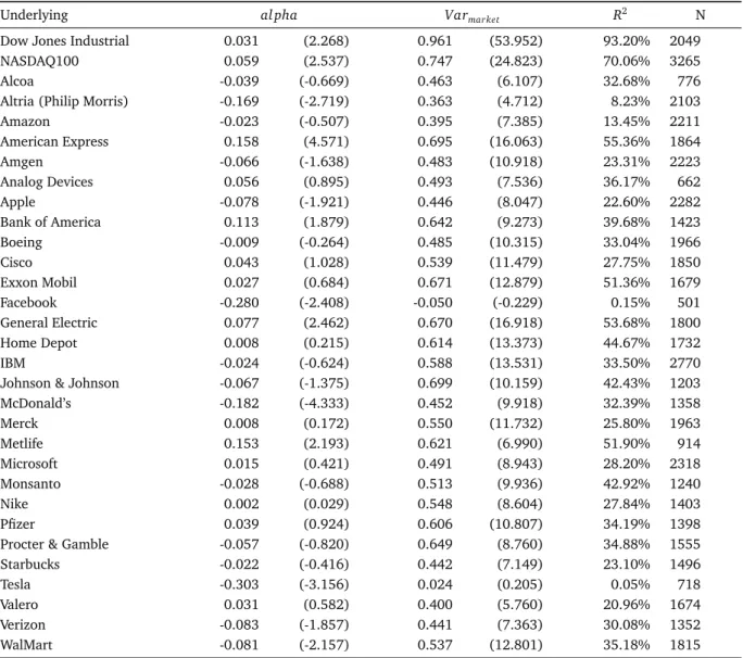
Since the results suggest that variance risk premia are deed significantly different from zero and negative for all in-dices and the majority of single names, but differ substan-tially in their absolute magnitude, the analysis is continued with an attempt to link the variance risk premium, or vari-ance swap returns, to the underlying’s exposure to system-atic variance. For this purpose, I compute a variance beta that measures the covariation between the return variance of a proxy for the market portfolio and that of the under-lying under consideration. Variance swap returns are then regressed on this variance beta. Because this analysis reveals that the variance beta can only explain variance swap returns for the US indices but not for single stocks, it is further ex-amined whether variance swap returns can be explained by a systematic variance risk factor that is proxied by the return on a variance swap with the S&P 500 as underlying. The underlying rationale for this course of action is that different studies find evidence that idiosyncratic return variances have a tendency to move together and possibly exhibit a common
factor structure (Herskovic et al.(2014)) to which a
diversi-fied index, however, should not be exposed. Investors may require compensation for the risk associated with common
movements in idiosyncratic return variances and this com-pensation may contribute to the observed variance risk
pre-mium (Schürhoff and Ziegler(2011),Gourier(2015)).
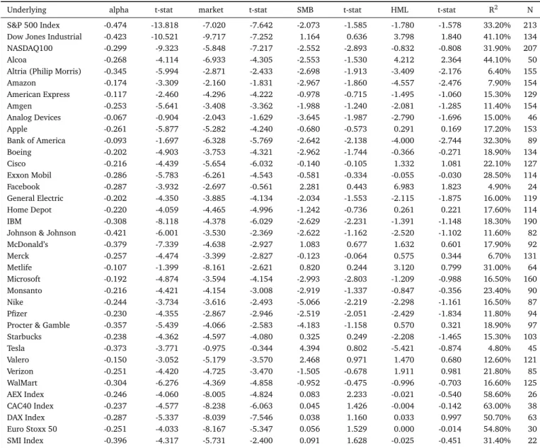
In order to further investigate whether return variance constitutes an independently priced risk factor, it is examined whether the classical Capital Asset Pricing Model (CAPM)
or theFama and French(1993) three-factor model are able
to explain variance swap returns. Even though both mod-els generate significantly negative regression betas with re-spect to market excess returns that are consistent with the commonly observed negative correlation between equity
re-turns and return variance (Glosten et al.(1993)), regression
alphas are mostly negative and significantly different from zero, which is suggestive of one or more additional priced risk factors.
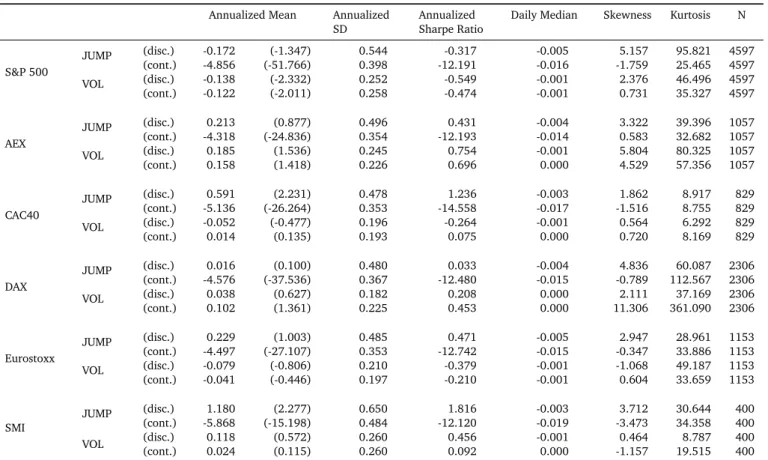
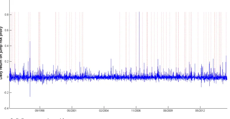
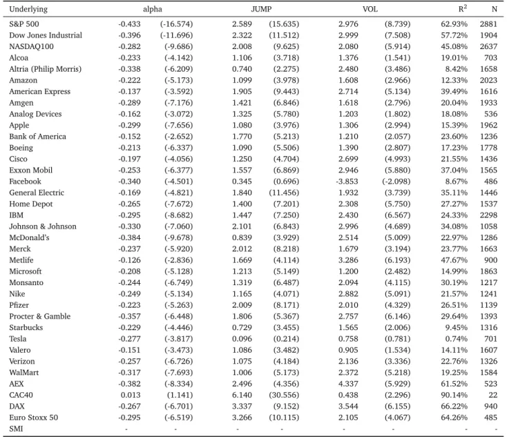
Because the total return variance reflects the continuous, i.e. pathwise variation as well as discontinuous price move-ments or jumps, I attempt to examine whether the risk asso-ciated with each of these types of price variation separately commands compensation that contributes to the observed variance risk premium. For this purpose I construct two risk-factor-mimicking portfolios from traded options that are tar-geted at offering exposure to one risk while being relatively unaffected by the other. Since the validity of any conclusion about the extent to which jump risk is priced crucially de-pends on the ability of the jump-risk-mimicking portfolio to reliably capture the exposure to jumps, it is tested whether positive returns on this factor coincide with jumps detected
by the non-parametric jump detection test ofLee and
Myk-land(2008), which appears to be the case. Even though both
constructed risk factors significantly contribute to explaining variance swap returns and continue to be significant when commonly used risk factors are included as control variables, abnormal returns remain mostly negative and significantly different from zero. Due to this, I consider the effect of the chosen specification of variance swap returns. In the initial setting, regressions are performed using continuously com-pounded variance swap returns to account for the substan-tial skewness and kurtosis in the distribution of raw returns. However, this has the drawback of shifting the mean return further into the negative domain, which may contribute to the persistently negative alphas. Due to this, robustness tests with raw variance swap returns instead of continuously com-pounded returns are performed and suggest that the specifi-cation has a certain impact on results but abnormal returns, especially for the US indices, often remain significant.
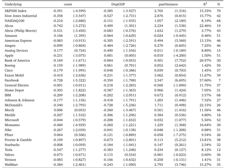
Finally, motivated by a relatively recent study by
Drech-sler(2013) who finds that model uncertainty can help
sub-stantially to explain the magnitude of the observed variance risk premium, I examine the relation between a proxy for model uncertainty and variance swap returns.
2. Literature review
For one thing, this work is related to prior studies that ex-amine whether a variance risk premium exists and in partic-ular to studies that examine the existence of the variance risk
premium not only for stock indices but also for single stocks. One of the earlier studies that provide empirical evidence for the existence of a negative variance risk premium in index
options is the work byBakshi and Kapadia(2003) in which a
long call option is dynamically hedged with the underlying. Since this strategy is effectively market-neutral and should
therefore only be exposed to volatility risk, Bakshi and
Ka-padia(2003) interpret the negative average returns on the strategy as evidence for the existence of a negative volatil-ity risk premium. While the outlined approach allows to
in-fer the variance risk premium rather indirectly,Carr and Wu
(2009) are among the first who use a model-free approach
to synthesize variance swap rates from a sample of traded options on five US stock indices and 35 individual stocks in order to examine the existence and dynamics of the vari-ance risk premium. This model-free approach allows a direct quantification of the variance risk premium which is defined as the difference between the risk-neutral expected and sub-sequently realized variance. Their results suggest that aver-age variance risk premia are negative and substantial for the five indices whereas premia for individual stocks exhibit con-siderable variation, are not always significant and can even be positive. They further examine whether observed vari-ance risk premia are related to a systematic varivari-ance factor proxied by the return variance of the S&P 500. This analysis reveals that assets with higher exposure to the variance fac-tor are associated with more negative variance risk premia, which leads them to conclude that investors dislike elevated levels of market volatility and are willing to accept negative average returns on variance swaps to insure against rising
market volatility. Moreover, Carr and Wu(2009) find that
frequently used asset pricing models such as the Capital
As-set Pricing Model or theFama and French(1993) model are
unable to explain variance swap returns.
Driessen et al.(2009) use the same model-free approach to derive variance risk premia embedded in S&P 100 stock index options and options on all its individual constituents.
Similar toCarr and Wu(2009), they find a significantly
nega-tive variance risk premium for the S&P 100 whereas the vari-ance risk premiums on individual stocks are often zero or even positive. Since an index variance risk premium should reflect the variance premia of all its constituents, they con-clude that a negative variance risk premium for the index together with non-existent or even positive variance risk pre-mia on its constituents is only reconcilable with priced corre-lation risk. In order to empirically test this hypothesis, they implement a trading strategy that is targeted at capturing the correlation risk premium and earns significant abnormal
returns. Based on their results, Driessen et al.(2009) also
link the expensiveness of index options relative to individ-ual stock options to the insurance against undesirable mar-ketwide correlation increases that index options offer but in-dividual options do not.
Schürhoff and Ziegler (2011) also synthesize variance swap rates to decompose total variance risk and examine the separate pricing of systematic and idiosyncratic variance risk for the S&P 100 and NASDAQ 100 index and all index
con-stituents. Consistent with previous findings, their results sug-gest that systematic variance carries a negative risk premium. Moreover, they also find that common idiosyncratic variance risk, i.e. the risk of comovements in the variances of idiosyn-cratic stock returns, carries a risk premium which is, on av-erage, positive. Since the total variance risk premium is the
sum of the two components,Schürhoff and Ziegler (2011)
argue that the non-existent variance risk premium on
indi-vidual stocks documented byDriessen et al.(2009) is due to
the fact that the two components offset each other for S&P 100 constituents. They further attribute the positive risk pre-mium on common idiosyncratic variance risk to financial in-termediaries that are net-long in options on individual stocks. Since these intermediaries are not able to perfectly hedge op-tions and are exposed to the associated idiosyncratic variance risk, they require compensation for upholding this position.
Moreover, with regard to the results byDriessen et al.(2009),
Schürhoff and Ziegler(2011) argue that the return on disper-sion trading strategies that target to capture the correlation risk premium does not represent compensation for the pure risk of marketwide increases in correlation but rather reflects a combination of risk premia on systematic variance and com-mon idiosyncratic variance risk.
In a related study, Gourier (2015) introduces an affine
jump-diffusion model that considers the factor structure of asset returns as well as that of idiosyncratic return variance, in which variance swap rates and the variance risk premium
– using the same definition asCarr and Wu(2009) – can be
derived in closed-form. Further analyses show that model-based variance swap rates match synthetic variance swap
rates remarkably well.Gourier(2015) finds a negative
vari-ance risk premium for all stocks that rises in absolute mag-nitude when the time to maturity increases. In contrast to
Schürhoff and Ziegler(2011), she further finds that idiosyn-cratic variance risk carries a negative risk premium whose contribution to the overall variance risk premium is substan-tial and amounts to 80% on average.
The presented selection of studies shows that the exis-tence of a negative variance risk premium for stock indices is well documented whereas the results and in particular the sign of the variance risk premium for single stocks are more ambiguous.
Apart from studies that document the existence of a vari-ance risk premium, this work is also related to studies that attempt to examine whether the wedge between risk-neutral expected and actually realized variances predominantly re-flects the risk that arises from stochastic volatility or rather results from compensation for the risk of discontinuous price
movements, i.e. price jumps. For instance,Todorov(2010)
examines the dynamics of the variance risk premium over time and especially how it is related to price jumps. For this purpose he fits a general semiparametric stochastic volatil-ity model to S&P 500 data and uses deep out-of-the-money and close-to-maturity options to estimate the risk-neutral tail jump intensity. The chosen approach allows him to infer the contribution of stochastic volatility and jumps to the ex-ante variance risk premium which he measures as the difference
between a model-based estimate for the future expected vari-ance under the physical measure and the VIX index. He con-cludes that jumps play a crucial role in explaining the vari-ance risk premium. Since it increases after the occurrence of price jumps and reverts only slowly to its long-run mean thereafter whereas the impact of jumps on future market dy-namics is limited, he concludes that investors’ perception of jump risk is time-varying.
In a related work,Bollerslev and Todorov(2011) employ
extreme value theory together with high frequency and op-tions data in a nonparametric setting to decompose the eq-uity risk premium and the variance risk premium into two separate components for diffusive and jump risk. Their re-sults suggest that on average approximately 5% (in absolute terms) of the equity risk premium and more than half of the variance risk premium represent compensation for jump tail events.
3. Theoretical foundation of the variance risk premium
For a negative risk premium, such as the observed vari-ance risk premium, to persistently occur, two complementary forces that are outlined in the following must coincide. First, the party requiring the risk premium must be exposed to es-sentially non-diversifiable, i.e. systematic, or non-hedgeable risk since otherwise a risk premium would not be justified and competitors would underbid each other until the mar-ket price of the asset equals its no-arbitrage price. The ex-istence of such a non-diversifiable or non-hedgeable risk is strongly linked to the assumed price process of the underly-ing. It is well known that if the price of the underlying is assumed to follow a Geometric Brownian motion with
con-stant return variance, as in the model byBlack and Scholes
(1973), markets are essentially complete and options are
re-dundant securities because any option can be perfectly repli-cated by holding the commensurate amount of the underly-ing and the risk-free bond. The crucial aspect of such a set-ting is that the option’s systematic risk is fully accounted for by the price of the underlying used in the replicating
port-folio (Hull(2009)). Thus, in a world such as that described
by Black and Scholes (1973), any exposure to options can be hedged perfectly and, if there is a competitive market for options, option prices should be solely determined by no-arbitrage conditions without the explicit consideration of risk premia. If stochastic volatility or random jumps in the asset price process are introduced, however, there are two addi-tional variables that can change randomly and affect the price of an option. Consequently, it is no longer possible to per-fectly replicate an option’s payoff and thus hedge the option through simple trading in the underlying and the risk-free
bond. As proven byBajeux-Besnainou and Rochet(1996),
in-troducing stochastic volatility that fluctuates independently of the price of the underlying (in contrast to a setting where volatility is a deterministic function of the asset price (e.g.
Dupire(1994))) in a continuous time setting makes a clas-sical European option always a non-redundant security. Be-cause neither stochastic volatility nor jumps are traded assets,
the market is incomplete with respect to states in the world
where these variables change (Staum (2007)). Technically,
market incompleteness means that there is no unique equiv-alent martingale measure, or risk-neutral probability distri-bution, for which all discounted asset prices are martingales,
but multiple such measures exist (Bajeux-Besnainou and
Ro-chet(1996)). Due to the absence of assets that allow to trade
these particular risks, it is also not possible to complement the underlying and the risk-free bond with an additional as-set whose price exclusively depends on these variables and thereby replicate and hedge the option perfectly. As a conse-quence, the holder of an option position is left with the essen-tially non-hedgeable risk of random changes in the variance of the underlying or price jumps and associated changes in the value of her option. Thus, depending on whether these additional sources of risk are systematic and therefore cor-related with aggregate consumption, they may command a
risk premium. For instance, in the model proposed byHull
and White(1987)), stochastic volatility does not carry a non-zero risk premium because it is explicitly assumed to be un-correlated with aggregate consumption. Likewise, for exam-pleMerton (1976) assumes that the source of price jumps is company- or industry-specific information so that the con-tribution of price jumps to stock returns is non-systematic. However, there is considerable empirical evidence that re-turn variances of different stocks tend to move together (e.g.
Andersen et al.(2001)) and correlations in changes of im-plied volatilities make it difficult to eliminate vega risk by
simple diversification (Engle and Figlewski(2014)). Thus,
it can reasonably be assumed that variance risk is system-atic and difficult to diversify. As a consequence, options will be priced to reflect the required compensation for random
changes in the volatility (e.g. Bates(2000)). Similarly,Ang
and Chen(2002) examine how correlations differ for upside and downside moves and find that correlation asymmetries are more pronounced for extreme downward moves, which can be interpreted as an indirect indication that jump risk may be systematic, thus potentially justifying a jump risk pre-mium.
Note that for example in the model by Heston (1993),
an additional option that is already traded would complete
the market (Staum(2007)) and theoretically allow to
per-fectly hedge the risk of random changes in return variance. However, even in this situation, a perfect hedge still requires that the applied option pricing model be correct and the cor-rect input parameters be used to reliably estimate each op-tion’s sensitivity with respect to random changes in the return variance. This leads to the closely related practical problem
of model uncertainty. In this contextBroadie et al. (2009)
argue that market makers in option markets may require a risk premium since the necessary estimation of parameters such as the spot volatility, long-run mean levels of volatility and volatility mean reversion parameters and the associated determination of hedge ratios in the presence of stochastic volatility and jumps is subject to considerable estimation risk and may lead to the effect that option market makers cannot
and Figlewski(1999) analyze the effect of inaccurate volatil-ity estimates on delta-hedged short positions in index options by comparing the performance using as input to the option pricing model the best historical estimate of volatility and actually realized volatility over the remaining life of the op-tion. Their results show that model risk due to an inaccurate volatility estimate has economically substantial effects even when positions are delta-hedged daily. Thus, the pricing of this estimation risk by risk-averse market makers could also contribute to the observed difference between option-implied and realized variances.
Empirical evidence that option market makers may
in-deed find it difficult to hedge their inventory is given by
Gâr-leanu et al.(2009) who argue that option prices should not be affected by demand pressures when competitive interme-diaries can hedge their option positions perfectly. They for-malize in a model the notion that risk-averse intermediaries require compensation for their inability to hedge their ex-posure and link the amount of unhedgeable risk to the net-position these market makers hold. Their empirical results suggest that option expensiveness, defined as the difference between the average of options’ implied volatility and a vola-tility forecast is indeed related to the net-position market makers have in options. In particular, index options in which intermediaries are net-short so that increases in volatility are associated with losses to the intermediary are visibly more expensive than individual equity options in which
interme-diaries are net-long. Further, Fournier and Jacobs (2015)
also assume that market makers face unhedgeable risks and find that an option market makers’ increasing inventory ex-posure to market variance risk, which is measured as the
ag-gregate Black and Scholes (1973) vega, is associated with
a significantly more negative variance risk premium (using the same definition of the variance risk premium as applied
here). In this context, the results ofGârleanu et al.(2009)
andFournier and Jacobs (2015) offer an interesting expla-nation for the differential magnitude of variance risk pre-mia in equity index options and options on individual stocks
(e.g. Carr and Wu(2009),Driessen et al.(2009)) with
re-gard to the net-position held by market makers in these con-tracts. Note, however, that the cited studies take the demand for options as exogenously given. Thus, they offer a poten-tial explanation for why market makers may demand a vari-ance risk premium but leave open the question why investors should be willing to pay it. This leads to the second prereq-uisite for the persistent existence of a variance risk premium. While market makers seem to be exposed to unhedgeable systematic risk which justifies a risk premium, the second pre-requisite for its persistent existence is that the assets on which an investor pays the premium, namely (index) options and variance swaps, offer insurance against an undesirable state of the world. If this was not the case, investors would not be willing to pay the substantial negative premium that is of-ten found. A risk-averse investor is usually characterized by marginal utility that decreases with wealth. Due to the asym-metry of changes in utility that result from positive and neg-ative changes in wealth or consumption of equal magnitude
with a concave utility function, a risk-averse individual will always be willing to give up wealth in the good state of the world, i.e. reduce current consumption, and pay insurance against realization of the bad state in which wealth is low and marginal utility is high. In this context, the apparent question is what exactly causes the risk-neutral expected variance to frequently exceed the realized variance. A possible
explana-tion is a phenomenon called asymmetric volatility (e.g. Wu
(2001)) that describes a negative correlation between market
returns and return variance. Due to this negative correlation, variance swaps naturally offer insurance against substantial market declines, which may explain why investors are willing to pay a premium for such instruments, i.e. accept a variance strike that is too high relative to the variance one would ex-pect to realize under the physical measure.
Moreover, a randomly changing return variance also im-plies that an investor’s final wealth is not only risky but also
ambiguous1or uncertain and there is empirical evidence of
ambiguity aversion, i.e. that people prefer to act on known
rather than on unknown probabilities (Ellsberg(1961)2).
An interesting and intuitive explanation how model un-certainty, which is closely linked to ambiguity aversion, can also help to explain risk-neutral expected variances that
fre-quently exceed realized variances is offered by
Drechsler (2013). He develops a model in which the rep-resentative investor has a reference model about the evolu-tion of certain economic fundamentals but is not confident whether this model is indeed correct. To account for this sit-uation and to derive decisions that are robust to model un-certainty, the investor considers alternative models that are statistically difficult to distinguish from the reference model and evaluates his decisions under the model which represents the “worst case”. The investor is particularly concerned that the reference model underestimates the intensity and mag-nitude of potential jumps. Thus, the risk-neutral probabili-ties that are determined under this “worst case” model are tilted toward states of the world in which wealth is low and marginal utility is high, in particular to states in which large negative jumps in the expected growth rate of cash flows oc-cur. As such important shocks to the economic state affect as-set prices and thus return variance, this mechanism directly translates into a higher risk-neutral expected variance. Be-cause, irrespective of the sign, the realized return variance is positively affected by the occurrence of jumps, a variance swap obviously offers insurance against such adverse move-ments. Moreover, an implication of this model is that the
1Risk refers to a situation in which possible outcomes are uncertain but
the distribution of outcomes is known. In contrast, ambiguity refers to a situation in which the outcome itself as well as the distribution of outcomes is not known (e.gAnderson et al.(2009)).
2Ellsberg(1961) describes a situation in which people can choose a ball
to be drawn from two different urns that contain red and black balls. A certain prize is received if a red ball is drawn and a smaller prize if a black ball is drawn. Urn I contains exactly 100 balls but nothing is known about the relative proportion of red and black balls. Urn II contains exactly fifty black and fifty red balls. Once asked to bet on the outcome that a red (black) ball will be drawn, the majority of people prefer Urn II (Urn I) over Urn I (Urn II).
magnitude of the variance risk premium depends on the de-gree of investors’ uncertainty. A circumstance that gives sup-port to this model is that, once calibrated, it is able to gen-erate the variance risk premium with a comparatively low level of risk aversion and to capture additional features of
asset returns.3 This is mainly a result of the explicit
consid-eration of model uncertainty. In a related model byDrechsler
and Yaron(2011) where this model uncertainty is not consid-ered and the variance risk premium only arises from shocks to long-run consumption growth, larger jumps and a higher risk aversion are necessary to produce results that match im-portant properties of the data. What both models (and many others) have in common, however, is that jumps are typically needed to produce variance risk premia that are close to the data estimates.
4. Methodology and data
4.1. Theoretical basis for extracting the risk-neutral expected variance
In this section, the methodology that is used to extract the risk-neutral expected variance from a set of traded op-tions is outlined. The derivation of the risk-neutral expected
integrated variance goes back to the work ofDemeterfi et al.
(1999), Britten-Jones and Neuberger (2000),
Carr and Madan(1998) and others.Carr and Madan(1998) show that the integrated variance of the futures price process can be replicated through a static portfolio of European op-tions across a continuum of strike prices and dynamic hedg-ing in the underlyhedg-ing futures contract if continuous tradhedg-ing is possible, interest rates are constant and the underlying fu-tures price is a continuous semi-martingale. Their solution
builds on the work ofNeuberger(1994) who finds that the
payoff from delta-hedging a contract that pays the log of the spot price at maturity equals the difference between the real-ized variance and the variance assumed for hedging. More-over, this log contract can be replicated through a static
po-sition in options (Breeden and Litzenberger(1978)).
In particularCarr and Madan(1998) derive the following
expression for the time-0 conditional expectation of variance
of the futures price process over the time horizon[0,T]under
the risk-neutral probability measureQwhereFt denotes the
timetprice of the futures contract that expires at timeTand
RVt,Tdenotes the annualized realized variance over the time
horizon[t,T]. EQ 0[RV0,T] =EQ[ 2 T(l o g( F0 FT) + FT F0−1) − 2 T Z T 0 (1 F0− 1 Ft)d Ft] (1)
3In particular, the model is able to generate the high equity risk premium,
low risk-free rate, excess volatility of equity returns relative to fundamentals, a substantial variance risk premium that has predictive power for equity returns and a realistic implied volatility surface that captures the implied volatility skew for different maturities.
The second term on the right hand side of equation (1)
represents the payoff of a continuously rebalanced position in the underlying futures contract. The first term represents
a log contract that pays f(FT)at maturity. The final payoff
of this log contract can be expressed as the final payoff of a static portfolio of European out-of-the-money (OTM) put
and call options on the underlying futures contract4across a
continuum of strike prices K with expiration at time T where each option is inversely weighted by the square of its strike
price K. Thus, the expression shown in equation (2) can be
derived. EQ 0[RV0,T] = 2 TE Q[ Z F0 0 1 K2(K−FT) +d K + Z ∞ F0 1 K2(FT−K) +d K − Z T 0 (1 F0− 1 Ft )d Ft] (2)
Note that the terminal option payoff in equation (2) is
the payoff on European options on the futures contract. How-ever, since the options and the futures contract expire at time
T and the futures price has to equal the spot price at
ma-turity to prevent arbitrage, European options on the futures and options on the spot are effectively equivalent. Moreover, in a risk-neutral world, the drift of the futures price is zero when the money market account is taken as numeraire
im-plying that the futures price is a martingale (Carr and Madan
(1998)). Thus, the expected value from continuous trading
in the futures contract is zero so that the last term in the square brackets can be omitted.
Since the current price of any asset should equal the pres-ent value of future expected cash flows, the final payoff of the option portfolio can be rewritten as the terminal value of
the current price of the option portfolio. Thus, the time –t
conditional expectation of variance over a time horizon[t,T]
under the risk-neutral measure can be stated as
EQ t [RVt,T] =e rt,T(T−t) 2 T−t [ Z F0 0 1 K2Pt(K,T)d K+ Z ∞ F0 1 K2Ct(K,T)d K], (3)
wherert,T is the time-trisk-free rate over the time horizon
[t,T]andPt(K;T)andCt(K,T)are the time-tprices of
Eu-ropean put and call options on the spot with strike price K
that expire at timeT. Equation (3) also denotes the variance
4Carr and Madan(1998) formally show that any twice differentiable
payoff function, f(FT), of the terminal futures price can be re-written as f(FT) = f(κ) +f0(κ)[(FT−κ)+−(κ−FT)+] +
Rκ
0 f00(K)(K−FT)+d K+ R∞
κ f00(K)(FT−K)+d K. Setting the arbitrary parameterκequal toF0
strike in a variance swap contract that is initiated at timet
and expires at timeT.
Equation (3) measures the risk-neutral expected variance
exactly when the price of the underlying evolves according to a purely continuous price process without jumps.
How-ever, Jiang and Tian (2005) show that this expression also
yields an accurate estimate under more realistic assumptions when the asset price process is allowed to exhibit jumps and the effect of implied jumps is included in the above measure so that an estimate of the total quadratic variation can be
obtained. Further, Carr and Wu (2009) show in a
simula-tion study that the jump-induced error is typically very small. In general, the approximation error due to jumps, i.e. the difference between the “true” risk-neutral expected variance
and the estimate obtained from equation (3) will be positive
when negative jumps dominate and can become significant when jumps significantly contribute to overall volatility,
pre-sumably in times of stress (Du and Kapadia(2011)).
Moreover note that equation (3) theoretically captures
the risk-neutral integrated variance of the futures price pro-cess. However, under the assumption of deterministic in-terest rates and dividend yields, the spot and futures price should have the same quadratic variation. Moreover, since interest rates are at historically low levels for a substantial pe-riod covered by the dataset and the time horizon over which the risk-neutral expected variance is approximated is rela-tively short (22 trading days), a violation of these assump-tions would probably have no significant effect on the results. Following the convention to determine the payoff on a
vari-ance swap that is described byAït-Sahalia et al.(2015b), the
annualized realized variance over the 22 trading day
hori-zon[t,t+22], where t now denotes a specific trading day, is
defined as the annualized sum of daily squared log-returns
shown in equation (4) based on a day-count-convention of
255 business days per year. The spot price used in equation
(4) is adjusted for stock splits and spin-offs.
RVt,t+22=255 22 22 X i=1 (log( St+i St+i−1 ))2 (4)
As noted byBollerslev et al.(2011), the use of model-free
realized volatilities, computed by summing squared returns from high-frequency data, generally allows a more accurate ex post observation of historical volatility than the
expres-sion used in equation (4) and would therefore naturally lend
itself for an accurate measurement of the variance risk pre-mium as defined below. However, in an earlier version of
their study,Bollerslev et al.(2008) find, based on the model
ofHeston(1993), that the mean bias in the volatility risk pre-mium using model-free implied volatility and realized volatil-ity estimated from daily returns was only about 1.05% of the
theoretical volatility premium for a sample size of 600.5 I
consider this magnitude of bias sufficiently small to justify
5This can be seen by comparing the figures in Table1of their paper. The
mean bias in the volatility premium is about 0.0021 compared to a theoret-ical premium of -0.20.
the use of equation (4) to measure the realized variance over
the relevant horizon.
4.2. The variance risk premium
FollowingCarr and Wu(2009), the variance risk premium
is defined as the difference between the actually realized
vari-ance over the time horizon[t,T]and the time-texpected
vari-ance under the risk-neutral measure over that same time
pe-riod, i.e. VRPt,T =RVt,T−EQ
t [RVt,T]. In this sense,VRPt,T·
100 is the payoff in monetary units to an investor who holds a long position in a variance swap contract with notional
100 that is initiated at timetand expires at timeT, whereas
RVRPt,T = RVt,T
EQ t[RVt,T] −
1 is the excess return to the investor when the variance swap rate is thought to be the initial
in-vestment. LVRPt,T = log(RVt,T/EQt[RVt,T]) can therefore be
regarded as the continuously compounded excess return on this variance swap contract.
When no confusion arises, I drop subscripts in the text.
Specifically, I use VRP, RVRP and LVRP to refer to VRPt,T,
RVRPt,T andLVRPt,T in the text.
4.3. Data
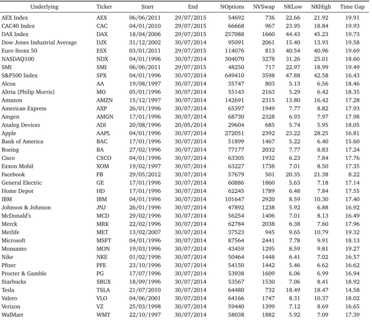
The applied dataset includes daily option price informa-tion on three US and five European stock indices as well as 29 single stocks from the US. A detailed overview of the in-cluded indices and stocks along with further information is
shown in Table1below.
Daily settlement as well as bid and ask prices for options on European indices as well as the corresponding index se-ries and all overnight indexed swap (OIS) rates are retrieved from Thomson Reuters Datastream. Bid and ask prices of options on US indices and stocks, the corresponding prices of the underlyings and the London Interbank Offered Rate (LIBOR) curve are retrieved from OptionMetrics. For the Eu-ropean indices, OIS rates are used as proxy for the risk-free rate. For the US underlyings, LIBOR rates are used as prox-ies for the risk-free rate prior to 2007 whereas from the year 2007 on, OIS rates are used as a proxy. The reason for this change is that derivative dealers generally used LIBOR as a proxy for the risk-free rate prior to 2007 but have switched to OIS rates for collateralized transactions in later years as a consequence of substantial rises in LIBOR rates during the
financial crisis (Hull and White(2015)). Since the data used
here stem from options traded on organized exchanges with central clearing authorities and collateral requirements, the application of these rates appears to be a reasonable choice. If available, option prices for subsequent analyses are de-fined as the average of bid and ask prices. Otherwise, the daily settlement price is used. To obtain the final data sam-ple, several exclusionary criteria are applied to the initial set of options. First, if applicable bid prices are required to be strictly positive and bid-ask-spreads to be equal or greater than zero. Second, options with less than seven days to matu-rity are excluded since prices of such options might be biased
Table 1: Data description
Note: Entries list the name of included stocks and indices as well as their tickers which are sometimes used in other tables to reference the respective underlying. Start and End denote the first and last day in the sample on which a valid estimate of the variance risk premium could be obtained. NOptions denotes the number of option quotes available after filters are applied. NVSwap denotes the number of days on which a valid estimate for the VRP could be obtained. NKLow and NKHigh denotes the average daily number of options with expiration dateTLandTH, respectively, from which implied volatilities could
be derived and interpolated. TimeGap denotes the average distance in days betweenTLandTHover which the risk-neutral expected variance is interpolated.
A description ofTLandTHis given in section 4.4.
Underlying Ticker Start End NOptions NVSwap NKLow NKHigh Time Gap AEX Index AEX 06/06/2011 29/07/2015 54692 736 22.66 21.92 19.91 CAC40 Index CAC 04/01/2010 29/07/2015 66668 967 23.95 18.84 19.93 DAX Index DAX 18/04/2006 29/07/2015 257088 1660 44.43 45.23 19.73 Dow Jones Industrial Average DJX 31/12/2002 30/07/2014 95091 2061 15.40 13.93 19.58 Euro Stoxx 50 ESX 03/01/2011 29/07/2015 114076 813 40.54 40.96 19.69 NASDAQ100 NDX 04/01/1996 30/07/2014 304070 3278 31.26 25.01 18.60
SMI SMI 06/06/2011 29/07/2015 48250 717 22.97 18.99 19.49
S&P500 Index SPX 04/01/1996 30/07/2014 649410 3598 47.88 42.58 16.43
Alcoa AA 19/08/1997 30/07/2014 35747 803 5.13 6.56 18.46
Altria (Philip Morris) MO 05/01/1996 30/07/2014 55143 2163 5.29 6.42 18.35 Amazon AMZN 15/12/1997 30/07/2014 142691 2315 13.80 16.42 17.28 American Express AXP 26/01/1996 30/07/2014 65397 1949 7.77 8.82 17.93 Amgen AMGN 17/01/1996 30/07/2014 68730 2328 6.93 7.97 17.98 Analog Devices ADI 20/08/1996 20/05/2014 29604 685 5.74 5.95 18.05 Apple AAPL 04/01/1996 30/07/2014 272051 2392 23.22 28.25 16.81 Bank of America BAC 17/01/1996 30/07/2014 51899 1467 5.22 6.40 15.60
Boeing BA 27/02/1996 30/07/2014 77177 2032 7.77 8.83 17.24
Cisco CSCO 04/01/1996 30/07/2014 63305 1932 6.23 7.84 17.76 Exxon Mobil XOM 19/02/1997 30/07/2014 63227 1738 7.01 8.50 17.35 Facebook FB 29/05/2012 30/07/2014 57679 501 20.35 21.38 8.22 General Electric GE 17/01/1996 30/07/2014 60886 1860 5.63 7.18 17.14 Home Depot HD 17/01/1996 30/07/2014 62245 1789 6.48 7.84 17.55
IBM IBM 04/01/1996 30/07/2014 101647 2920 8.59 10.30 17.40
Johnson & Johnson JNJ 26/01/1996 30/07/2014 47892 1238 5.92 6.88 16.92 McDonald’s MCD 29/02/1996 30/07/2014 56254 1406 7.01 8.13 16.49 Merck MRK 22/02/1996 30/07/2014 62784 2038 6.38 7.60 17.96 Metlife MET 13/02/2007 30/07/2014 37523 945 9.65 10.79 19.32 Microsoft MSFT 04/01/1996 30/07/2014 87564 2441 7.78 9.91 18.13 Monsanto MON 19/03/1996 30/07/2014 43459 1295 8.59 9.81 19.27 Nike NKE 01/02/1996 30/07/2014 50464 1448 6.41 7.02 16.57 Pfizer PFE 23/10/1996 30/07/2014 54150 1442 5.46 6.62 16.62 Procter & Gamble PG 17/07/1996 30/07/2014 53938 1609 6.06 6.99 16.94 Starbucks SBUX 18/09/1996 30/07/2014 53567 1530 7.06 8.41 18.92 Tesla TSLA 21/07/2010 30/07/2014 64480 732 18.49 18.47 14.58 Valero VLO 04/06/2001 30/07/2014 64166 1747 8.31 10.37 18.02 Verizon VZ 25/03/1998 30/07/2014 59440 1399 7.12 8.69 16.65 WalMart WMT 22/10/1997 30/07/2014 58038 1882 5.92 7.09 17.39
(Jiang and Tian(2005)). Third, index options with zero trad-ing volume are excluded from the dataset because the prices
of such options may not reflect true value (Jiang and Tian
(2005)). Since most single stock options are less frequently
traded than index options, a less strict criterion is applied to such options in that only options with zero trading volume and open interest smaller than 100 contracts are excluded.
Since the following applications require a dividend yield for the indices of which a reliable estimate is difficult to ob-tain, the option-implied dividend yield is obtained through a combined application of the put-call parity and spot-futures
parity. In a first step, the time-toption-implied price, Fti, of
the futures contract that expires at timeTis inferred through
put-call-parity (e.g. Hull(2009)) that is shown in equation
(5).
Fti=K+ert,T(T−t)·(C
t(K,T)−Pt(K,T)) (5)
In order to select the put and call option used in equation
(5), the methodology applied by the Chicago Board Options
Exchange for calculating its volatility index (CBOE(2015))
is used. For every maturity on a given day, the pair of op-tions with the same strike price and maturity for which the
absolute price difference is smallest is used in equation (5).
over the time horizon[t,T], θt,T, is then extracted through
the spot-futures parity (e.g. Hull(2009)) that is shown in
equation (6).
Fti=Ste(rt,T−θt,T)(T−t) (6)
The outlined procedure ensures that the option pair used in the estimation of the implied dividend yield consists of at-the-money (ATM) options which are, especially for the in-dices considered here, typically relatively liquid. Thus, prices of such options and derived implied dividend yields can
gen-erally be expected to be reliable. Nevertheless,
option-implied dividend yields are occasionally negative. Such neg-ative values occur remarkably often during times of finan-cial turmoil, espefinan-cially during October 2008 and November 2011. Due to this, the negative yields most likely capture the effect of a discount rate used by market participants that exceeds the rate that is used to derive the implied dividend yield. Even though these negative dividend yields ensure that put-call parity is technically satisfied, it is obviously implau-sible to us them for further applications. Thus, the following adjustments are made to replace negative values: whenever possible, a replacement value for a negative forward looking dividend yield at a given maturity is obtained through lin-ear interpolation or extrapolation of implied dividend yields at adjacent maturities on the same day. If a linear interpo-lation or extrapointerpo-lation is not possible because the number of positive implied dividend yields at different maturities is smaller than two on a given day, the implied dividend yield for the same expiration date on the previous day is used as a replacement value. If none of these two adjustments results in a positive value or no value can be found, the implied div-idend yield is set to zero. For those observations where the implied dividend yield is replaced, a new forward price corre-sponding to the adjusted implied dividend yield is computed. For stocks a similar procedure is applied with the excep-tion that the implied present value of dividends is derived instead of an implied dividend yield.
After the derivation of implied dividend yields and present values of dividends, a fourth exclusionary criterion is applied
before implied volatilities are derived. As outlined by
Aït-Sahalia and Lo (1998), in-the-money (ITM) options are traded relatively infrequently compared to ATM or OTM op-tions. Therefore, prices of such options, and implied volatili-ties derived from these prices, tend to be unreliable. For this reason, ITM options are removed from the dataset.
For European options, implied volatilities are inferred
based on the model ofBlack and Scholes(1973) (henceforth
referred to as B-S model).6 For American options, implied
volatilities provided by OptionMetrics are used. For such op-tions, OptionMetrics uses a binomial tree approach account-ing for the effect of the early exercise premium.
6This is done with an adjusted version of Mark Whirdy’s code ”Fast
Matrixwise Black-Scholes Implied Volatility” for Matlab that is available under the following address: http://www.mathworks.com/matlabcent ral/fileexchange/41473-fast-matrixwise-black-scholes-impli ed-volatility.
Index options with implied volatilities greater than 80% and single stock options with implied volatilities greater than 100% are removed from the dataset. Such observations are probably outliers that would corrupt the implied volatility surface.
In addition to the options data, price information from the Center for Research in Security Prices, factor returns from Kenneth French’s website and data from the Survey of Pro-fessional Forecasters, which are introduced in detail when applied, are used.
4.4. Implementation of the method to extract the risk-neutral expected variance
In order to obtain an estimate of the risk-neutral expected
variance over the time horizon[t,T], equation (3) is
numer-ically evaluated using the trapezoidal method. A practical
problem arises since equation (3) requires an infinite
num-ber of options across a continuum of strike prices whereas the number of traded options is finite. To cope with this situ-ation, I generate 5000 artificial options that expire at the two
expiration dates TL and TU closest below and aboveTover
an equally-spaced range of strike prices of±8 standard
devi-ations from the current spot price. This standard deviation is estimated as the average of the implied volatilities of the two options that are closest to being at-the-money and expire at
time TL. In a simulation based on a model with stochastic
volatility and jumps,Jiang and Tian(2005) show that
trun-cation errors are generally negligible if the truntrun-cation points, i.e. the highest and lowest observed strike prices, are more than two standard deviations from the current forward price,
F0, and can be further reduced by applying the extrapolation
scheme outlined below. They further show that discretiza-tion errors resulting from non-continuous strike prices are negligible when the gap between consecutive strike prices is smaller than or equal to 0.35 standard deviations. Thus,
5000 options over a range of strike prices between±8
stan-dard deviations from the current spot should help to alleviate truncation and discretization errors.
In order to generate the artificial option prices, implied volatilities are needed. As noted in section 4.3, implied vola-tilities for European options are obtained based on the model byBlack and Scholes(1973) whereas implied volatilities pro-vided by OptionMetrics are used for American options. For
any given day t and the two expiration dates TL and TU,
implied volatilities are then interpolated across moneyness,
defined as k ≡ log(K/Fti), between the highest and lowest
observed strike price using cubic splines. Jiang and Tian
(2007) argue that the use of cubic splines leads to the
conve-nient property that the implied volatility function is smooth over the range of observed strike prices, which is a direct
implication of no-arbitrage constraints (e.g. Breeden and
Litzenberger (1978)). For strike prices below the smallest and above the highest observed strike price, implied
volatil-ity is held constant at the value observed at these end points.7
extrapo-The prices of artificial European options that expire at time
TL andTU over the continuum of strike prices are obtained
by inserting the interpolated implied volatilities into the B-S-formula. In the next step these option prices are used to
numerically evaluate equation (3) and obtain an estimate of
the risk-neutral expected variances over the two time
hori-zons [t,TL]and[t,TU]. An estimate of the risk-neutral
ex-pected variance over the desired horizon [t,T], can then be
obtained through linear interpolation between the expected
risk-neutral variances over the time horizons [t,TL]
and[t,TU]. Note that, in order to ensure that the
interpo-lation and extrapointerpo-lation scheme can work properly and de-rived estimates of the risk-neutral expected variance are reli-able, this procedure is only applied on days on which at least four traded options are available. Moreover note that the B-S model is only used as a convenient way to derive implied volatilities from and translate implied volatilities into options prices. In particular, it is not assumed that this model is a true representation of reality.
A description of the average time over which the risk-neutral expected variance is interpolated along with the
av-erage number of options that expire at times TL and TH is
shown in Table1.
5. Empirical analysis
5.1. Realized variance risk premia
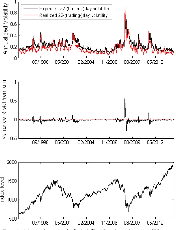
Figure 1 plots the daily time series of annualized
risk-neutral expected and actually realized volatilities over the subsequent 22 trading days, the variance risk premium,
de-fined asVRPt,T, and the index level for the S&P 500 index
between January 4th1996 and July 30th2014. From Figure
1 it is evident that the approximation of the expected
ance captures the dynamic of the subsequently realized vari-ance quite well and that substantial changes in the varivari-ance risk premium go hand in hand with significant fluctuations in the index level. This is also confirmed by the high correla-tion coefficient of 0.6437 between risk-neutral expected and subsequently realized variance for the S&P 500 index. At the same time, however, the wedge between the two variance measures is also apparent. For most of the time, the vari-ance risk premium is negative and relatively stable but expe-riences substantial fluctuations when major market changes occur and reaches unprecedented levels during the financial crisis.
Table 2 shows summary statistics for the variance risk
premium over a 22 trading day horizon in three different
forms, defined either as the time series average of VRPt,T·
lation scheme where the slope of the extrapolated segment is set equal to the slope of the interior segment at the endpoints. Even though this procedure better captures the observed skew in implied volatility surfaces for certain strike sections, it can lead to the implausible drawback that further-out-of-the-money call options have higher artificial prices than nearer-out-of-the-money call options, which occasionally happens here. Thus, the constant extrapolation scheme with zero slope is applied.
100,LVRPt,T orRVRPt,T. The reason for introducing a
loga-rithmic version of the variance risk premium is that the VRP and RVRP distributions exhibit substantial skewness and kur-tosis, indicating that the two stem from a highly non-Gaussian distribution, while LVRPs generally appear more normal which might be beneficial for subsequent regression analy-ses.
Consistent with previous studies, the mean VRP is neg-ative on all stock indices and statistically significantly dif-ferent from zero at the 1%-level for the S&P 500, the AEX, and the Euro Stoxx 50 and significant at the 5%-level for the Dow Jones and NASDAQ 100. Only for the Swiss SMI and the DAX, the variance risk premium is not significant on any conservative level. The distributions of both, VRP and RVRP show substantial kurtosis and positive skewness and are re-flective of high and positive returns which fatten the right tail of the distributions. In contrast, LVRPs exhibit a consid-erably lower skewness and kurtosis, which is due to the fact that especially the excessively high, positive returns during the recent financial crisis are alleviated through the logarith-mic transformation. In this context, it is also noticeable that the standard deviations of the VRPs are excessive, especially for single stocks, which partly explains why the VRP is statis-tically different from zero only for comparatively few stocks. Indeed, even though VRP is negative in most cases, the null hypothesis that realized and expected risk-neutral variances do not differ on average cannot be rejected at the 5% signif-icance level for 21 of the 29 stocks.
Mean LVRPs are negative for all underlyings and
t-statis-tics8are generally higher. The mean LVRP is significantly
dif-ferent from zero at the 1%-level for all underlyings.
How-ever, as pointed out byDriessen et al. (2009), a necessary
remark in this context is that due to the concavity of the logarithmic function, Jensen’s inequality implies that mean log variance risk premia are negative even under the null hy-pothesis of equality between risk-neutral expected and subse-quently realized variance. When raw variance swap returns
(RVRPt,T = RVt,T
EQ[RVt,T]−1) are used instead, mean returns are
generally smaller in absolute magnitude than for the LVRPs but still negative for 35 underlyings. However the mean raw return is statistically significantly different from zero at the 5%-level for only 14 underlyings.
Qualitatively, the results in the left panel of Table 2 are
similar to those obtained byCarr and Wu(2009) who find
sig-nificantly negative variance risk premia for stock indices but only comparatively few single stocks for which the premia are significant. Despite this tendency, the results are quite
different from those ofDriessen et al.(2009) who find a
sig-nificantly negative variance risk premium for the S&P 100 index but no evidence for the presence of a generally neg-ative variance risk premium in individual constituents.
In-8Except for equation (9), all t-statistics and regressions, as well as
stan-dard deviations adjusted according to the method ofNewey and West(1987) are obtained using Kevin Sheppard’s MFE Toolbox for Matlab throughout this work. The toolbox is available underhttp://www.kevinsheppard.com/ MFE_Toolbox.
Figure 1: Time series of risk-neutral expected and realized volatility, variance risk premium and the S&P 500
Note: The first plot shows the time series of annualized risk-neutral expected and subsequently realized volatility over 22 trading days in the period from January 4th1996 to July 30th2014 for the S&P 500 Index. Both measures are annualized on a basis of 255 trading days in a year. The second plot shows the
realized variance risk premium over 22 trading days,VRP0,T, over the corresponding sample period. The red horizontal line indicates a VRP equal to zero.
T able 2: Summary statistics of variance risk premia Note: Entries refer to the time period from January 4 th 1996 until July 29 th 2015. R V and EV denote the realized and risk-neutral expected variance, respectively . R ealized volatility is calculated from daily returns and annualized by p 255 / 22. t-stat denotes the rele vant t-statistics adjusted for serial correlation according to the method by Newey and W est (1987) with a lag length of 22 days. Sample std., Skew , and K urt denotes the sample standard deviation, skewness and kurtosis. Sharpe ratio is the annualized Sharpe ratio calculated as the annualized mean LVRP or R VRP divided by the corresponding sample standard deviation adjusted for serial dependence according to Newey and W est (1987) with 22 lags and annualized by p 255 / 22. Descriptive statistics of variance risk premia VRP as ( R V − E V ) · 100 LVRP as ln(R V / EV) R VRP as R V / EV -1 T icker R ealized volatility Mean t-stat Sample std. Skew K urt Mean t-stat Sample std. Skew K urt Sharpe Ra-tio Mean t-stat Sample std. Skew K urt Sharpe Ra-tio N AEX 16.12% -0.68 -3.01 2.18 1.22 8.51 -0.32 -4.61 0.59 0.43 3.27 0.58 -0.12 -1.70 0.65 2.56 11.20 0.11 736 C AC 19.88% -0.62 -1.93 3.38 2.30 12.56 -0.27 -4.61 0.57 0.45 3.40 0.50 -0.09 -1.35 0.66 2.99 16.70 0.07 967 D AX 20.21% -0.84 -1.65 5.78 4.02 37.84 -0.34 -6.46 0.61 0.50 3.85 0.54 -0.12 -1.91 0.74 3.51 19.47 0.06 1660 DJX 15.17% -0.84 -1.99 4.95 4.92 51.04 -0.50 -10.72 0.58 0.74 5.04 0.80 -0.25 -4.63 0.67 4.46 28.23 0.14 2061 ESX 19.60% -0.95 -3.02 2.88 1.30 7.73 -0.33 -5.05 0.55 0.27 2.96 0.60 -0.15 -2.60 0.53 1.91 7.70 0.18 813 NDX 26.05% -1.17 -2.52 7.38 3.17 24.10 -0.33 -10.68 0.51 0.59 4.65 0.64 -0.17 -4.55 0.60 4.50 33.35 0.13 3278 SMI 14.05% -0.24 -0.65 3.06 3.18 16.51 -0.33 -4.26 0.64 0.91 4.36 0.54 -0.08 -0.68 0.93 3.61 17.74 0.03 717 SPX 17.10% -1.25 -3.65 5.15 5.72 60.03 -0.54 -15.05 0.57 0.79 5.07 0.85 -0.29 -6.61 0.67 5.61 46.08 0.14 3598 AA 40.18% -0.37 -0.17 21.06 6.71 58.86 -0.22 -3.99 0.55 0.67 4.81 0.48 -0.04 -0.51 0.77 3.93 22.72 0.03 803 MO 25.68% -1.16 -1.79 9.53 2.97 27.06 -0.37 -7.32 0.71 0.42 4.46 0.54 -0.07 -0.78 1.25 8.63 96.92 0.01 2163 AMZN 47.01% 1.65 1.01 24.60 2.74 14.05 -0.23 -5.31 0.62 0.45 3.91 0.38 -0.01 -0.23 0.86 4.11 27.72 0.01 2315 AXP 35.11% 1.13 0.90 15.47 4.26 26.86 -0.18 -4.34 0.57 0.64 4.44 0.33 0.00 0.01 0.80 3.53 18.79 0.00 1949 AMGN 32.06% -1.54 -2.12 10.51 1.42 12.37 -0.30 -7.05 0.59 0.10 2.95 0.50 -0.12 -2.83 0.59 2.17 10.59 0.10 2328 ADI 51.22% 0.52 0.17 23.07 2.16 10.88 -0.19 -3.19 0.49 0.20 3.35 0.41 -0.06 -0.94 0.53 2.11 9.26 0.07 685 AAPL 39.31% -1.31 -0.63 39.51 14.80 242.03 -0.31 -8.64 0.54 0.80 7.11 0.60 -0.11 -1.76 1.15 14.55 275.48 0.04 2392 BAC 39.00% 7.30 1.52 46.18 5.19 31.82 -0.19 -3.42 0.61 0.77 4.64 0.30 0.03 0.36 0.98 4.54 32.94 -0.01 1467 BA 28.94% -1.35 -2.45 7.92 2.96 27.29 -0.26 -7.18 0.51 0.26 4.00 0.54 -0.12 -3.16 0.56 3.80 29.38 0.14 2032 C SCO 39.36% -0.11 -0.10 14.34 1.92 10.54 -0.24 -5.38 0.62 0.29 3.22 0.42 -0.04 -0.73 0.72 2.55 11.85 0.02 1932 X OM 22.53% -0.33 -0.33 12.02 9.05 98.71 -0.31 -6.73 0.57 0.72 5.26 0.55 -0.11 -1.45 0.90 7.55 84.13 0.04 1738 FB 43.97% -2.21 -0.68 19.40 1.88 8.67 -0.25 -2.60 0.60 0.88 4.22 0.40 -0.03 -0.23 0.85 3.19 13.74 0.01 501 GE 30.84% -0.82 -1.03 10.46 2.38 17.44 -0.23 -5.83 0.54 0.59 4.45 0.46 -0.06 -1.12 0.73 4.26 29.99 0.04 1860 HD 30.48% -0.80 -1.01 12.18 7.80 93.72 -0.32 -7.60 0.55 0.49 4.77 0.61 -0.13 -2.54 0.78 7.69 87.12 0.09 1789 IBM 26.61% -1.32 -3.14 6.87 1.22 12.72 -0.34 -9.08 0.58 0.22 3.21 0.57 -0.15 -4.08 0.58 2.49 12.76 0.13 2920 JNJ 19.07% -1.26 -2.61 5.81 2.82 23.23 -0.43 -7.77 0.64 0.21 3.97 0.75 -0.19 -3.35 0.72 5.24 44.45 0.16 1238 MCD 18.85% -1.29 -3.28 4.68 1.67 26.08 -0.41 -9.26 0.50 0.69 3.82 0.84 -0.24 -5.43 0.50 3.07 17.35 0.30 1406 MRK 26.06% -0.81 -1.47 8.06 2.71 22.74 -0.29 -6.57 0.63 0.32 2.98 0.50 -0.08 -1.67 0.70 2.37 10.97 0.06 2038 MET 34.99% 1.02 0.35 30.18 10.83 140.21 -0.22 -4.11 0.53 1.35 9.33 0.46 -0.02 -0.16 1.28 9.28 104.98 0.00 945 MSFT 32.20% -0.81 -1.20 9.94 3.09 20.24 -0.24 -6.53 0.55 0.34 3.39 0.45 -0.08 -1.86 0.62 2.71 14.56 0.06 2441 MON 32.56% -1.04 -0.81 13.47 5.17 42.87 -0.29 -6.24 0.50 0.53 4.07 0.59 -0.14 -2.68 0.55 2.83 13.40 0.14 1295 NKE 29.08% -0.99 -1.25 9.93 2.60 16.39 -0.31 -6.18 0.61 0.41 3.36 0.55 -0.10 -1.77 0.70 2.86 13.87 0.07 1448 PFE 27.28% -1.32 -3.05 6.10 1.90 13.01 -0.30 -6.50 0.56 -0.01 3.78 0.58 -0.13 -2.96 0.56 2.56 13.24 0.16 1442 PG 21.38% 0.87 0.50 18.83 8.20 75.10 -0.39 -6.31 0.68 1.03 5.98 0.54 -0.06 -0.44 1.44 7.22 62.59 0.01 1609 SBUX 33.55% -0.39 -0.43 12.89 4.39 37.57 -0.26 -5.59 0.56 0.51 3.28 0.49 -0.08 -1.67 0.65 2.77 14.51 0.07 1530 TSLA 54.35% -5.68 -2.16 22.93 1.66 6.89 -0.32 -4.59 0.60 0.31 2.74 0.58 -0.12 -1.71 0.61 1.85 6.57 0.11 732 VLO 38.84% 0.12 0.08 17.15 5.42 44.52 -0.18 -4.17 0.52 0.48 3.68 0.34 -0.03 -0.62 0.62 2.68 13.15 0.02 1747 VZ 22.19% -1.31 -2.11 6.85 3.76 40.91 -0.33 -8.23 0.49 0.41 3.72 0.75 -0.18 -4.31 0.50 3.38 22.50 0.25 1399 WMT 24.47% -1.11 -2.31 6.02 1.09 12.29 -0.35 -8.19 0.54 0.32 3.30 0.64 -0.17 -4.20 0.54 2.56 12.94 0.18 1882
deed, the mean VRP is significantly negative at the 5%-level for only 7 of 129 (5%) stocks in their sample whereas this is the case for 9 of 29 stocks (31%) here. In this context, it is necessary to point out that the 29 stocks in this dataset have specifically been selected according to the number of price quotes provided by OptionMetrics and the number of valid price quotes following the criteria outlined above to allow the computation of a high number of estimates of the risk-neutral expected variance. Options that are comparatively illiquid and thus carry a substantial illiquidity premium should trade at lower prices, which would directly translate into lower im-plied volatilities. Applying the same procedure to derive the risk-neutral expected variance to such options should then naturally lead to lower expected risk-neutral variances and, holding realized variance constant, to less negative or even positive variance risk premia. Thus, the results here do not
necessarily contradict the findings byDriessen et al.(2009)
but could simply reflect different sample selection criteria and resulting differences in the sample composition.
When turning to the profitability of variance swap invest-ments, the results show that the average continuously com-pounded return on shorting a 22-day variance swap on one of the major indices over the entire sample period is in the range of 27% in case of the CAC40 to 54% in case of the S&P 500. In this context, it is noticeable that the average returns on single stock variance swaps are lower than those on some indices, especially the US indices, but not substantially lower. However, even though the variance premia are substan-tial, they are relatively low compared to the figures found by other studies. This circumstance is most obvious when one turns to the left panel of Table 2 where the payoff on a long variance swap for a notional of 100 currency units is shown.
For instance, Carr and Wu(2009) find average payoffs of
$2.5 and above for the S&P 500, the Dow Jones and NAS-DAQ. The lower payoffs over the entire sample might in part be due to the fact that especially during the financial crisis in 2008 and 2009 and its aftermath, realized variance has
fre-quently and substantially exceeded expected variance.9 This
observation is also in line with the argument ofCarr and Lee
(2009) who point out that short positions in variance swaps
led to significant and unprecedented losses especially during the final quarter of 2008. They further outline that market makers’ difficulty to hedge their exposure to variance swaps, in particular for single names, led to a complete collapse of the single name variance swap market in 2009. For the sake of completeness, however, it is necessary to point out that the variance risk premia obtained here are generally smaller, in absolute terms, even over the same time period covered by
Carr and Wu(2009).
9In addition, the smaller variance risk premiums found here compared to
those found byCarr and Wu(2009) on the same data are due to the different interpolation schemes. WhileCarr and Wu(2009) use a linear interpolation scheme, the cubic spline interpolation applied here usually leads to lower implied volatilities and therefore lower option prices since the typical shape of implied volatilities across moneyness is convex. However, as shown below, the influence of the interpolation scheme is comparatively small.
In order to evaluate the profitability of variance swap in-vestments with regard to their risk-return profile Table 2 also shows the annualized Sharpe Ratios. Since a variance swap contract is essentially a forward contract that does not tie up capital until maturity, the given variance swap returns di-rectly represent excess returns and the Sharpe Ratios are sim-ply computed as the annualized average return on the vari-ance swap divided by the annualized return standard devia-tion which is again adjusted for serial correladevia-tion according
to the method ofNewey and West(1987). Considering the
risk-return trade-off of shorting a 22-day variance swap, the high Sharpe Ratios for LVRPs of up to 0.85 for the S&P 500
index are relatively close to the estimates of Carr and Wu
(2009) and suggest that variance swaps can be attractive
in-vestments. The premia that investors are obviously willing to pay for holding long variance swaps appear substantial com-pared to the risk to which the short side is exposed. However, when one considers the right panel in Table 2 for RVRPs, it is apparent that the high Sharpe Ratios for the LVRPs are mainly the result of the logarithmic transformation which not only alleviates the effect of large positive returns and thereby re-duces the mean but also lowers the standard deviation. Both effects cause the Sharpe Ratios from shorting variance swaps to be substantially higher for LVRPs.
Of course, the extent to which the reported results are reflective of the profitability of actual variance swap invest-ments crucially depends on how well the synthetic variance swap rates approximate the prices of actually traded
instru-ments. However, at least for the S&P 500 index,Aït-Sahalia
et al.(2015b) find that the methodology applied here leads to synthetic variance swaps rates for maturities of up to six months that are roughly in line with those of actually traded instruments.
As outlined before, the unprecedented levels of realized variance that manifested during the financial crisis also led to previously unseen returns on variance swaps. In order to evaluate the extent to which these returns affect the re-sults reported in Table 2, Table A1 shows the same
descrip-tive statistics for the time period from January 4th1996 until
December 31st 2007. For most underlyings the payoffs on
a variance swap per 100 currency units notional is slightly higher in absolute terms than for the entire sample, whereas the continuously compounded returns as well as the raw re-turns are comparable and sometimes even lower in absolute terms than for the entire sample. The comparable mean re-turns over the two different samples can be explained by the fact that a long position in a variance swap earned substan-tial positive returns during the turmoil of 2008. However, after return variances had exploded, the variance swap rates increased accordingly and remained at their elevated levels even when realized variances reverted to lower levels so that average returns appear to be relatively unaffected over the entire sample period. This pattern is also apparent in the first plot in Figure 1. With regard to the relatively stable av-erage variance swap returns, it is obvious that the Sharpe Ratios which are higher compared to those over the entire sample period for LVRPs as well as for RVRPs are