Syracuse University
Syracuse University
SURFACE
SURFACE
Electrical Engineering and Computer Science -
Technical Reports
College of Engineering and Computer Science
12-1-2011
Outlier detection using modified-ranks and other variants
Outlier detection using modified-ranks and other variants
Huaming Huang
Syracuse UniversityKishan Mehrotra
Syracuse University, [email protected]
Chilukuri K. Mohan
Syracuse University, [email protected]
Follow this and additional works at: https://surface.syr.edu/eecs_techreports Part of the Computer Sciences Commons
Recommended Citation
Recommended Citation
Huang, Huaming; Mehrotra, Kishan; and Mohan, Chilukuri K., "Outlier detection using modified-ranks and other variants" (2011). Electrical Engineering and Computer Science - Technical Reports. 72.
https://surface.syr.edu/eecs_techreports/72
This Report is brought to you for free and open access by the College of Engineering and Computer Science at SURFACE. It has been accepted for inclusion in Electrical Engineering and Computer Science - Technical Reports by an authorized administrator of SURFACE. For more information, please contact [email protected].
SYR-EECS-2011-12
December 01, 2011
Outlier Detection Using Modified-ranks and Other Variants
Huaming Huang
Kishan Mehrotra
Chilukuri K. Mohan
ABSTRACT
:
Rank-based algorithms provide a promising approach for outlier detection, but currently used
rank-based measures of outlier detection suffer from two deficiencies: first they take a large value from an
object near a cluster whose density is high even through the object may not be an outlier and second the
distance between the object and its nearest cluster plays a mild role though its rank with respect to its
neighbor. To correct for these deficiencies we introduce the concept of modified-rank and propose new
algorithms for outlier detection based on this concept. Our method performs better than several density-based
methods, on some synthetic data sets as well as on some real data sets.
KEYWORDS
:
Outlier detection, ranking, neighborhood sets, clustering
Syracuse University - Department of EECS,
4-206 CST, Syracuse, NY 13244
(P) 315.443.2652 (F) 315.443.2583
Outlier Detection Using Modified-ranks and
Other Variants
Technical Report Number: SYR-EECS-2011-12
Huaming Huang, Kishan Mehrotra, Chilukuri K. Mohan
Department of EECS, Syracuse University
Abstract. Rank-based algorithms provide a promising approach for outlier detection, but currently used rank-based measures of outlier de-tection suffer from two deficiencies: first they take a large value for an object near a cluster whose density is high even through the object may not be an outlier and second the distance between the object and its nearest cluster plays a mild role though its rank with respect to its neighbor. To correct for these deficiencies we introduce the concept of modified-rank and propose new algorithms for outlier detection based on this concept. Our method performs better than several density-based methods, on some synthetic data sets as well as on some real data sets.
Keywords: Outlier detection, ranking, neighborhood sets, clustering.
1
Introduction
Outlier detection is an important task for data mining applications. Several effec-tive algorithms have been successfully applied in many real-world applications. Density-based algorithms such as ”local outlier factor” (LOF) and connectivity-based outlier factor (COF) were proposed by [1] and [7] respectively. Jinet al.[5] proposed another modification, called INFLO, which is based on a symmetric neighborhood relationship. Tao and Pi [8] have proposed a density-based clus-tering and outlier detection (DBCOD) algorithm. Outliers detection based on clustering has been proposed in the literature, see Chandola et al. [3], where an object is declared as an outlier if it does not belong to any cluster. This in turn, requires a new clustering philosophy in which all objects of a given data set are not required to be a cluster. Tao and Pi’s [8] clustering approach belongs to this category. In this paper we modify their approach towards this goal, but we differ in the outlier detection step; we use clustering to eliminate the objects that are not suspected outliers and evaluate outlierness of the remaining objects only.
Another rank based detection algorithm (RBDA) was recently proposed by Huang et al.[?]. It was observed that RBDA demonstrates superior performance than LOF, COF, and INFLO. However, RBDA is found to assign a large out-lierness value to an object in the vicinity of a large cluster, although the object may not be an outlier. In this paper we present few approaches to rectify this deficiency of RBDA — first is a simple modification to RBDA whereas in the
second and third approaches the size of the cluster is explicitly addressed; in all cases clustering acts as a preprocessing step.
The paper is organized as follows. In Section 2, after introducing key no-tations and definitions, we briefly describe RBDA and DBCOD. In Section 3, first we illustrate the above described weakness of RBDA followed by suggested measures of outlier detection. These new measures are compared with RBDA and DBCOD using one synthetic and three real data sets. Brief descriptions of data sets and a summary of our findings are presented in Section 4, followed by the conclusions and future work.
2
Notation and Definitions
In following notations and concepts are used throughout the paper.
2.1 Notation
– Ddenotes the given dataset of all observations.
– d(p, q) denotes the distance between two points p, q ∈ D. This distance measure could be any appropriate distance but for concreteness we use the Euclidean distance.
– dk(p) = the distance betweenpand itskth nearest neighbor,kis a positive
integer.
– Nk(p) = {q ∈ D − {p} : d(p, q) ≤ dk(p)} denotes the set of k nearest
neighbors ofp.
– rq(p) denotes the rank of pamong neighbors ofq∈ Nk(p); i.e., rq(p) is the
rank ofd(q, p) in{d(p, o) :O∈D− {q}}.
– RNk(p) ={q: q∈D andp∈ Nk(q)} denotes the set of reversek nearest
neighbors ofp.
2.2 Definitions
The following definitions are used in the proposed clustering algorithm; all def-initions are relative with respect to a positive integer `. In other words, for example, D-reachable defined below should be viewed as D-reachable given `
D-reachable – An object p is directly reachable (D-reachable) from q, if p ∈ N`(q).
Reachable – An objectpis reachable from q, if there is a chain of objects p≡
p1, . . . , pn≡q, such that pi is D-reachable frompi+1for all values of i.
Connected – If pis reachable from q, and q is reachable fromp, then pand q
are connected.
Neighborhood Clustering – A subsetC of D is a cluster of non-outliers if the following three conditions are satisfied:
2. Forp∈C,pis D-reachable from at least two other objects inC.
3. |C| ≥ m∗, where m∗ is the minimum number of objects in a cluster, it is pre-defined by users (domain experts).
Condition 3 above is used to avoid treating a small number of outliers as a cluster. We denote the clustering method asN C-clustering; more formally asN C(`, m∗). For instance,N C(6,5) means that a cluster contains connected objects for `=6 and a cluster must contain at least 5 objects.
The values of`andm∗ are mainly decided based on domain knowledge. If`
is smallN C-clustering method will find small and tightly connected clusters and large value of ` will find large and loose clusters. If the clusters are small and tight, we expect to find more objects that don’t belong to any cluster whereas in the latter case, only a few objects will be declared as outliers. In real world applications (such as credit card fraud detection) most of the transactions are normal and only 0.01% or less of the transactions are fraudulent. In this case, a small value of`is more suitable than a large`.
The value ofm∗ has a similar effect: ifm∗ is too small, then the cluster size may also be too small, and a small collection of outliers may be considered as a cluster, which is not what we want. In our experiments, m∗ is set to a fixed value of 6.
RBDAis a rank-based outlier detection approach that identifies outliers based on mutual closeness of a data point and its neighbors. Forp, q∈D, ifq∈ Nk(p)
andp∈ Nk(q), then pand qare ”close” to each other. To capture this concept
we define a measure of ”outlierness” ofp, as follows:
Ok(p) =
P
q∈Nk(p)rq(p)
|Nk(p)| .
IfOk(p) is ‘large’ thenpis considered an outlier.
Density-based clustering and outlier detection algorithm (DBCOD)
Forp∈D Tao and Pi [8] define the local density, the neighborhood-based den-sity factor, and neighborhood-based local denden-sity factor of p, respectively, as:
LDk(p) = P q∈Nk(p) 1 d(p,q) |Nk(p)| ,NDFk(p) = |RNk(p)| |Nk(p)| , and NLDFk(p) = LDk(p)×NDFk(p).
The threshold of NLDF, denoted as thNldf, is defined as:
thNldf =
mink(NLDFk(p)) if for all objectsp∈D,NDFk(p) = 1
maxk(NLDFk(p)) otherwise
Using the above definitions, Tao and Pi’s [8] find the clusters based on the definitions in section 2.2,except their definition of D-reachability is as follows:p
andqare in each other’sk-neighborhood and NLDFk(q)<thNldf. Points outside
3
Weighted RBDA and other improvements
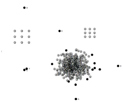
In general RBDA performs better than density-based algorithms such as LOF, COF and INFLO. A sample performance table is presented in Section 4. these density based measures do not assign appropriate measures of outlierness to one or two objects that are clearly far away from a cluster whereas RBDA is mostly successful. A simple example illustrates this observation. Consider the synthetic dataset in Figure 1. This dataset contains two clusters of different densities and an ‘outliers’ A. Fork= 5,6,7 or 8, the density-based algorithms such as LOF,
Fig. 1.Synthetic dataset-0 with one outlier, but LOF, COF and INFLO identify B as the most significant outlier.
COF and INFLO do not identify A as the most significant outlier. Instead, B is their top choice, which is wrong. Why B gets a higher outlier value? The reason is that some of B’sk-neighbors are from a high density cluster while the others are from a low density cluster and due to mix density of neighborhoods density-based algorithms fail to identify object A as an outlier. RBDA identifies the object A as the most significant outlier.
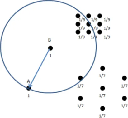
However, behavior of RBDA is also inconsistent with expectation when an object is near a dense cluster, which we identify as the‘cluster density effect’. Consider the data in Figure 2 where two points are of special interest; A in the neighborhood of a cluster with low density (25 objects) and B in the neighbor-hood of a cluster with high density (491 objects).
By visual inspection, it can be argued that the object ‘A’ is an outlier whereas object ‘B’ is a possible but not definite outlier. For k=20,O20(A)=25 because
rank of ’A’ is 25 from all of its neighbors. On the other hand, the ranks of ’B’ with respect to its neighbors are: 2, 8,. . . , 132, 205, 227; so thatO20(B) is 93.1.
RBDA concludes that ‘B’ is more likely outlier than ‘A’. It is clearly an artifact due to large and dense cluster in the neighborhood of ‘B’, i.e., a point closer to a dense cluster is likely to be misidentified as an outlier, even though it may not be. Such behavior of RBDA, due to cluster density, is observed for some values ofk.
Fig. 2. An example to illustrate ‘Cluster Density Effect’ on RBDA; RBDA assigns larger outlierness measure to B.
By visual inspection, we generally conclude that a point is an outlier if it is ‘far away’ from the cluster. This implies that the distance of the object (from the cluster) plays an important role; but accounted for in RBDA only through ranks. Perhaps this deficiency in RBDA can be fixed by incorporating distance in RBDA. The distance can be measured in many ways; either collectively for objects inNk(p) or by accounting for the distance of eachq∈ Nk(p) separately.
These different ways of accounting for distance lead to potentially many pos-sible measures of outlierness. We have explored some of them but in the next subsection we present only one that performed better than others.
3.1 Weighted RBDA
Rank-based approach ignores useful information contained in the distance of the object from other neighboring objects. To overcome the weakness of RBDA due to “cluster density effect”, we propose to adjust the value of RBDA by the average distance ofpfrom itsk−neighbors. Step by step description of this rank and distance based detection algorithm (RADA) is given below:
1. Choose three positive integersk, `, m∗. 2. Find the clusters inD byN C(`, m∗) method.
3. An object o is declared a potential-outlier if it is does not belong to any cluster.
4. Calculate a measure of outlierness: Wk(p) =Ok(p)×
P
q∈Nk(p)d(q,p)
|Nk(p)| .
5. Ifpis a potential-outlier andWk(p) is large, declarepis an outlier.
For the dataset in Figure 2 we observe that W20(A) = 484.82 and W20(B) =
396.19 implying that A is more likely outlier than B, illustrating that RADA is capable of fixing the discrepancy observed in RBDA.
3.2 Outlier detection using modified-ranks (ODMR)
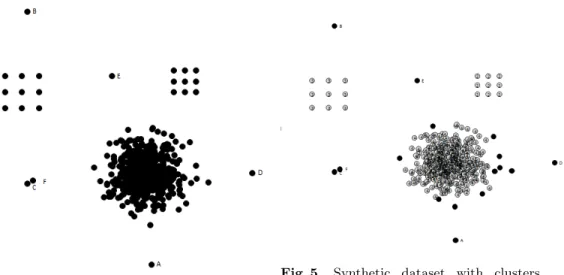
In this section we propose an alternative procedure to overcome the cluster density effect. We have observed that the size of neighboring cluster plays an
Fig. 3.Assignment of weights in different clusters and modified-rank (modified-rank ofA, with respect toB, is 1 + 1 + 5×1
9+ 1 7.)
important role when calculating the object’s outlierness via RBDA. To modify this effect, all clusters of all sizes are assigned equal weights (including isolated points viewed as a cluster of size 1) and all |C| observations of the cluster are assigned equal weights = 1/|C|.1The rankr
q(p) of an observationpis equal to
the number of points within a circle of radius d(q, p) centered at q. In RBDA we sum rq(p) for all values ofq∈ Nk(p). In the proposed version, we calculate
“modified-rank” ofp, which is defined as the sum of weights associated with all observations within the circle of radiusd(q, p) centered atq; that is
modified-rank ofpfromq=mrq(p) =
X
s∈{d(q,s)≤d(q,p)}
weight(s),
and sum the “modified-ranks” inq∈ Nk(p).
Figure 3 illustrates how modified-rank is calculated. Step by step description of the proposed method is as follows:
1. Choose three positive integersk, `, m∗.
2. Find clusters in D by N C(`, m∗). All objects not belonging to any cluster are declared as potential-outliers.
3. IfC is a cluster andp∈C, then the weight ofpisb(p) = |C|1 .
4. For p ∈ D and q ∈ Nk(p), Q denotes the set of points within a circle of
radiusd(q, p), i.e.,Q={s∈D|d(q, s)≤d(q, p)}. Then the modified-rank of
pwith respect toq, denoted asmrq(p), is computed asmrq(p) =Ps∈Qb(s).
5. For a potential outlier p, its ODMR-outlierness, denoted as ODMRk(p), is
defined as: ODMRk(p) =Pq∈Nk(p)mrq(p)
6. Ifpis a potential outlier and ODMRk(p) is large, we declarepis an outlier.
1
We have experimented with another weight assignment to points within a cluster, equal to 1/p|C|, but the results are not as good as when weights are 1/|C|.
3.3 Outlier detection using modified-ranks with distance (ODMRD)
Influenced by the distance consideration of section 3.1, in this section we present yet another algorithm that combines ODMA and distance. ODMRDk(p) is
ob-tained by implementing all steps as before except Step 5 of the previous algorithm is modified as follows:
(5*) For a potential outlierp, its ODMRD-outlierness, denoted as ODMRDk(p),
is defined as: ODMRDk(p) =Pq∈Nk(p)mrq(p)×d(q, p)
4
Experiments
4.1 Datasets
We use one synthetic and three real datasets to compare the performance of RBDA with RADA, ODMR, ODMRD and DBCOD.
Real Datasets Real datasets consist of iris, ionosphere, and Wisconsin breast cancer datasets obtained from UCI repository. The real datasets were used in two different ways, following the criterion used in [4],[7], and [2]:
1. By making a rare set out of one the class. (1) In the Iris dataset, which is a three-class problem and contains 150 observations equally divided in three classes, 45 observations were removed randomly from the iris-setosa class. (2) In the ionosphere dataset, which is a two-class problem, out of 126 ‘bad’ instances, 116 were randomly removed, leaving 10 ‘outliers’. (3) Finally, in the Wisconsin dataset, which is also a two-class problem and consists of 236 observations of benign and 236 observations of malignant cancer, after removing duplicates and observations with missing features, 226 malignant observations were removed, leaving 10 ‘outliers’.
2. By planting new observations in the existing datasets. These planted obser-vations are such that one or more features are assigned the extreme values. (1) In the Iris dataset three observations were planted, (2) in the ionosphere dataset three outliers were planted and (3) in the Wisconsin dataset two outliers were planted.
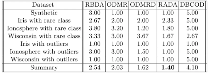
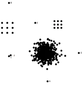
Synthetic datasets The synthetic datasets are two dimensional so that it is easy to see and interpret the results. Synthetic dataset consists of 515 instances including six planted outliers; has one large normally-distributed cluster and two small uniform clusters. This datasets is intended to test the algorithms’ ability to overcome the problem of “cluster density effect”. This dataset and clusters obtained by an application ofN C(6,6), are depicted in Figure 6.
4.2 Performance Measures
To measure the performance, three metrics are selected -mt, recall and RankPower,
[?]; briefly defined below. We listmmost suspicious objects in the datasetD, by a given outlier detection algorithm, which contains exactlydttrue outliers. Let
Fig. 4.Synthetic dataset
Fig. 5. Synthetic dataset with clusters found byN C(6,6); black object represents the outliers.
the algorithm producesmt(true) outliers out ofm. Suppose that the algorithm
assigns the rank Ri to theith outlier amongm, whereRi = 1 represents most
suspicious outlier and a larger value of Ri means that the algorithm considers
that the ith outlier is less suspicions. Based on these values the performance measures we consider are:
Recall = |mt| |dt| , RankPower = n(n+ 1) 2Pn i=1Ri .
RankPower summarizes the overall performance of an algorithm but an object by object assignment of ranks is naturally more illuminating.
4.3 Results
In this section we present a sample of results, extensive tables for all datasets for various values of m and k are available in the Appendix of the technical report [?]. Table1 compares RBDA with density based outlier detection methods LOF, COF, INFLO. Rank table of planted outliers in the synthetic dataset is presented in Table 2. In Table 3 we compare RBDA, ODMR , ODMRD, RADA , and DBCOD using RankPower for ionosphere dataset with rare class and in Table4 we summarize of RankPower for all datasets.
5
Conclusion
We observe that rank based approach is highly influenced by the density of neigh-boring cluster. Furthermore, by definition, ranks use the relative distances and
Table 1. Comparison of LOF, COF, INFLO and RBDA for k = 11, 15, 20 and 23 respectively for the Ionosphere dataset. Maximum values are marked as bold.
m LOF COF INFLO RBDA
Nrc Pr Re RP Nrc Pr Re RP Nrc Pr Re RP Nrc Pr Re RP 5 5 1.00 0.50 1.000 5 1.00 0.50 1.000 5 1.00 0.50 1.000 5 1.00 0.50 1.000 15 6 0.40 0.60 1.000 6 0.40 0.60 0.778 6 0.40 0.60 1.000 8 0.53 0.80 0.818 30 7 0.23 0.70 0.667 7 0.23 0.70 0.560 7 0.23 0.70 0.651 9 0.30 0.90 0.703 60 8 0.13 0.80 0.409 8 0.13 0.80 0.409 8 0.13 0.80 0.419 9 0.15 0.90 0.703 85 9 0.11 0.90 0.294 9 0.11 0.90 0.290 9 0.11 0.90 0.300 10 0.12 1.00 0.372
Table 2.Outliers detected by RBDA, ODMR, ODMRD, RADA, and DBCOD in the
synthetic dataset, fork= 25. Recall in this dataset the set of planted six outliers is S ={A, B,C, D, E,F}.
m RBDA ODMR ODMRD RADA DBCOD
6 {A,B,C,D,E,F} {A,B,C,D,E,F} {A,B,C,D,E,F} {A,B,C,D,E,F} {A,B,D}
Table 3.Performance measures of RBDA, ODMR , ODMRD, RADA , and DBCOD
for ionosphere dataset
m RBDA ODMR ODMRD RADA DBCOD
mt Re RP mt Re RP mtRe RP mt Re RP mt Re RP 5 5 0.5 1 5 0.5 1 5 0.5 1 5 0.5 1 0 0 0 15 8 0.80.783 8 0.80.783 8 0.8 0.818 8 0.8 0.818 0 0 0 30 9 0.90.703 9 0.90.682 9 0.9 0.726 9 0.9 0.726 0 0 0 60 9 0.90.703 9 0.90.682 9 0.9 0.726 9 0.9 0.726 9 0.90.091 85 10 1 0.369 10 1 0.364 10 1 0.390 10 1 0.387 10 1 0.098
Table 4.Summary of RBDA, ODMR, ODMRD, RADA and DBCOD for all
experi-ments.
Dataset RBDA ODMR ODMRD RADA DBCOD
Synthetic 3.00 1.00 1.00 1.00 5.00
Iris with rare class 2.67 2.00 2.00 2.33 5.00 Ionosphere with rare class 3.80 3.20 1.20 1.80 5.00 Wisconsin with rare class 3.33 3.00 3.67 1.67 2.67 Iris with outliers 1.00 1.00 1.00 1.00 1.00 Ionosphere with outliers 3.00 3.00 1.50 1.00 5.00 Wisconsin with outliers 1.00 1.00 1.00 1.00 5.00
Summary 2.54 2.03 1.62 1.40 4.10
Numbers in the table represent the average performance of the algorithms; a small value implies better performance.
ignore the ‘true’ distances between the observations. An outlier detection algo-rithm benefits from ‘true’ distance as well. Thus we introduce distance in RBDA and observe that the overall performance of RADA is much better than the orig-inal RBDA. That the ‘true’ distance plays an important role is further confirmed by the performance of the alternative algorithms ODMR and ODMRD; it is ob-served that in general ODMRD performs better than ODMR. We plan to further investigate the proposed algorithms for robustness and consistency.
A
Experiments Results
In this section, we will cover the detail about the datasets, and how we conduct the experiments.
A.1 Synthetic Dataset
Synthetic dataset consists of 515 instances including planted six outliers; has one large normally-distributed cluster and two small uniform clusters. It is the synthetic dataset that can be used to test the algorithms’ ability to overcome the problem of ”cluster density effect”. Four different values of k, 25, 35 and 50 are selected and m = 6, 10, and 16.
Fig. 6.Synthetic Dataset
The following figure shows the clusters and outliers found byN C(6,6). Black object represents the outlier object.
Forkis 25, 35 and 50, ODMR, ODMRD and RADA are the best algorithms since they all rank the six real outliers in their top 6 outputs. And DBCOD
Table 5.Rank table of comparison of RBDA,ODMR,ODMRD,RADA and DBCOD for 25, 35 and 50 respectively for synthetic dataset. Number in table represents the rank in the output by descending order.
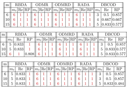
m RBDA ODMR ODMRD RADA DBCOD
6 A,B,C A,B,C A,B,C A,B,C A,B,D D,E,F D,E,F D,E,F D,E,F
m RBDA ODMR ODMRD RADA DBCOD
6 A,B,C A,B,C A,B,C A,B,C A,B,D D,F D,E,F D,E,F D,E,F
m RBDA ODMR ODMRD RADA DBCOD
6 A,B,C A,B,C A,B,C A,B,C A,B,D D,F D,E,F D,E,F D,E,F
Table 6.Comparison of RBDA, ODMR, ODMRD, RADA and DBCOD for k = 25,
35 and 50 respectively for synthetic dataset. Maximum values are marked as red.
m RBDA ODMR ODMRD RADA DBCOD
mt Re RP mt Re RP mt Re RP mt Re RP mt Re RP
6 6 1 1 6 1 1 6 1 1 6 1 1 3 0.5 0.857
10 6 1 1 6 1 1 6 1 1 6 1 1 4 0.667 0.667 15 6 1 1 6 1 1 6 1 1 6 1 1 5 0.833 0.577
m RBDA ODMR ODMRD RADA DBCOD
mt Re RP mt Re RP mt Re RP mt Re RP mt Re RP
6 5 0.833 1 6 1 1 6 1 1 6 1 1 3 0.5 0.857 10 5 0.833 1 6 1 1 6 1 1 6 1 1 5 0.833 0.577 15 6 1 0.808 6 1 1 6 1 1 6 1 1 5 0.833 0.577
m RBDA ODMR ODMRD RADA DBCOD
mt Re RP mt Re RP mt Re RP mt Re RP mt Re RP
6 5 0.833 1 6 1 1 6 1 1 6 1 1 3 0.5 0.857 10 5 0.833 1 6 1 1 6 1 1 6 1 1 3 0.5 0.857 15 5 0.833 1 6 1 1 6 1 1 6 1 1 5 0.833 0.484
Fig. 7.Synthetic dataset with clusters found byN C(6,6). Black object represents the outlier object.
gets the worst performance for all values of k. In general, RBDA works better than DBCOD but worse than the others. And the ODMR, ODMRD and RADA algorithms show the very good performance and excellent ability to overcome the problem of cluster density effect since all of them get the maximum RankPower and maximum recall for all values ofk.
A.2 Real Datasets:
We have used three well known datasets, namely the Iris, Ionosphere, and Wis-consin breast cancer datasets. We use two ways to evaluate the effectiveness and accuracy of outlier detection algorithms; (i) detect rare classes within the datasets (which has also been used by other researchers such as Fenget al.and Tang et al. [4, 6]) and (ii) plant outliers into the real datasets (according to datasets’ domain knowledge) and expect outlier detection algorithms to identify them.
A.3 Real Datasets with Rare Classes
In this sub-section, we compare the algorithms in detecting rare classes. A class is made ‘rare’ by removing most of its observations. In all cases, the value of k
is chosen between 1% to 10% percentage of the size of the dataset. Because the attributes are dependent, Mahalanobis distance is used to measure the distance between two points.
Iris Dataset The dataset is about iris plant and contains three classes: iris setosa, iris versicolour, iris virginica with 50 instances each. The iris setosa class is linearly separable from the other two classes, but the other two classes are not linearly separable from each other. We randomly remove 45 instances from iris-setosa class to make it ’rare’; remaining 105 instances are used in the final dataset. Three selected values ofkare 5, 7, 10. Tables summarize our findings.
Table 7.Comparison of RBDA, ODMR, ODMRD, RADA and DBCOD for k = 5, 7
and 10 respectively for the Iris dataset with rare class. Maximum values are marked as red.
m RBDA ODMR ODMRD RADA DBCOD
mt Re RP mt Re RP mt Re RP mt Re RP mt Re RP
5 1 0.2 0.2 3 0.6 0.75 3 0.6 0.75 1 0.2 0.2 0 0 0 10 4 0.8 0.37 5 1 0.652 5 1 0.714 5 1 0.429 1 0.2 0.125 15 5 1 0.385 5 1 0.652 5 1 0.714 5 1 0.429 4 0.8 0.2 20 5 1 0.385 5 1 0.652 5 1 0.714 5 1 0.429 4 0.8 0.2
m RBDA ODMR ODMRD RADA DBCOD
mt Re RP mt Re RP mt Re RP mt Re RP mt Re RP
5 3 0.6 0.75 4 0.8 1 4 1 0.833 3 0.6 0.857 0 0 0 10 5 1 0.714 5 1 0.882 5 1 0.882 5 1 0.714 1 0.2 0.125 15 5 1 0.714 5 1 0.882 5 1 0.882 5 1 0.714 4 0.8 0.2 20 5 1 0.714 5 1 0.882 5 1 0.882 5 1 0.714 4 0.8 0.2
m RBDA ODMR ODMRD RADA DBCOD
mt Re RP mt Re RP mt Re RP mt Re RP mt Re RP
5 5 1 1 4 0.8 1 4 0.8 1 5 1 1 0 0 0
10 5 1 1 5 1 0.938 5 1 0.882 5 1 1 3 0.6 0.231 15 5 1 1 5 1 0.938 5 1 0.882 5 1 1 5 1 0.288 20 5 1 1 5 1 0.938 5 1 0.882 5 1 1 5 1 0.288
Forkis 5, ODMRD is the best outlier detection algorithm, and ODMR is the second best. Forkis 7, ODMRD and ODMR both achieve the best performance. DBCOD has the worst RandPower and recall which means that it has the worst performance. For k is 10, RBDA and RADA work better than all others, and DBCOD is still the worst algorithm in this experiment.
Johns Hopkins University Ionosphere Dataset The Johns Hopkins Uni-versity Ionosphere dataset contains 351 instances with 34 attributes; all at-tributes are normalized in the range of 0 and 1. There are two classes labeled as good and bad with 225 and 126 instances respectively. There is no duplicate instances in the dataset. To form the rare class, 116 instances from the bad class are randomly removed. Final dataset has only 235 instances with 225 good and
10 bad instances. Four values ofk=11, 15, 20 and 23 are used and for different value ofkthemvalues also vary.
For k is 7, 11, 15, and 23, ODMRD works the best, and RADA performs the second best and only has a little gap of performance from ODMRD. When
k is 20, RADA is even better than ODMRD for m is 15, 30 and 60. RBDA works better than DBCOD algorithms, but it performs worse than the others. In general, ODMRD is the best outlier detection algorithm in this experiment.
Wisconsin Diagnostic Breast Cancer Dataset Wisconsin diagnostic breast cancer dataset contains 699 instances with 9 attributes. There are many duplicate instances and instances with missing attribute values. After removing all duplicate and instances with missing attribute values, 236 instances labeled as benign class and 236 instances as malignant were left. Total 226 malignant instances are randomly removed following the method proposed by Cao. The final dataset consists of 213 benign instances and 10 malignant instances in our experiments.
Fork is 7, RBDA and RADA both work the best. The DBCOD algorithm gets the best RankPower when m is 25, but it only detects 9 of 10 outliers and has the worst precision and recall. For other values ofm, it gets the worst RankPower.
Forkis 11, RADA achieves the best performance. DBCOD performs the second best. ODMRd works only better than RBDA.
For k is 22, DBCOD achieves the best performance for all values of m. And ODMR shows the second-best performance in five algorithms.
RADA shows the best performance and DBCOD gets the second best in this experiment.
A.4 Real datasets with planted outliers
Detecting rare class instances may not be adequate to measure performance of an algorithm designed to detect outliers; because it may not be appropriate to declare them as outliers. In experiments described in this subsection we plant some outliers into the real datasets according to datasets’ domain knowledge.
Iris plant dataset with Outliers Three outliers are inserted into IRIS dataset, that is, there are three classes with 50 instances each and 3 planted outliers. The first outlier has maximum attribute values, second outlier has minimum attribute values, and the third has two attributes with maximum values and the other two with minimum values. Three values ofk, 7, 10, and 15 are selected for this experiment.
It can be seen that all algorithms perform well in this experiment, and all get the best performance.
Table 8.Comparison of RBDA, ODMR, ODMRD, RADA and DBCOD for 7, 11, 15, 20 and 23 respectively for the Ionosphere dataset with rare class. Maximum values are marked as red.
m RBDA ODMR ODMRD RADA DBCOD
mt Re RP mt Re RP mt Re RP mt Re RP mt Re RP 5 5 0.5 1 5 0.5 1 5 0.5 1 5 0.5 1 0 0 0 15 8 0.80.783 8 0.80.783 8 0.8 0.818 8 0.8 0.818 0 0 0 30 9 0.90.703 9 0.90.682 9 0.9 0.726 9 0.9 0.726 0 0 0 60 9 0.90.703 9 0.90.682 9 0.9 0.726 9 0.9 0.726 9 0.90.091 85 10 1 0.369 10 1 0.364 10 1 0.390 10 1 0.387 10 1 0.098
m RBDA ODMR ODMRD RADA DBCOD
mt Re RP mt Re RP mt Re RP mt Re RP mt Re RP 5 5 0.5 1 5 0.5 1 5 0.5 1 5 0.5 1 0 0 0 15 8 0.8 0.818 8 0.8 0.818 8 0.8 0.818 8 0.8 0.818 0 0 0 30 9 0.90.703 9 0.90.703 9 0.9 0.726 9 0.9 0.726 0 0 0 60 9 0.90.703 9 0.90.703 9 0.9 0.726 9 0.9 0.726 9 0.90.098 85 10 1 0.372 10 1 0.374 10 1 0.393 10 1 0.387 10 1 0.105
m RBDA ODMR ODMRD RADA DBCOD
mt Re RP mt Re RP mt Re RP mt Re RP mt Re RP 5 5 0.5 1 5 0.5 1 5 0.5 1 5 0.5 1 0 0 0 15 8 0.80.818 8 0.80.818 8 0.8 0.837 8 0.8 0.837 0 0 0 30 9 0.90.714 9 0.90.703 9 0.9 0.738 9 0.9 0.738 0 0 0 60 9 0.90.714 9 0.90.703 9 0.9 0.738 9 0.9 0.738 9 0.90.104 85 10 1 0.377 10 1 0.382 10 1 0.407 10 1 0.401 10 1 0.111
m RBDA ODMR ODMRD RADA DBCOD
mt Re RP mt Re RP mt Re RP mt Re RP mt Re RP 5 5 0.5 1 5 0.5 1 5 0.5 1 5 0.5 1 0 0 0 15 8 0.80.837 8 0.80.818 8 0.80.837 8 0.8 0.857 0 0 0 30 9 0.90.738 9 0.90.726 9 0.90.738 9 0.9 0.75 0 0 0 60 9 0.90.738 9 0.90.726 9 0.90.738 9 0.9 0.75 9 0.90.106 85 10 1 0.387 10 1 0.39 10 1 0.414 10 1 0.414 10 1 0.114
m RBDA ODMR ODMRD RADA DBCOD
mt Re RP mt Re RP mt Re RP mt Re RP mt Re RP 5 5 0.5 1 5 0.5 1 5 0.5 1 5 0.5 1 0 0 0 15 8 0.80.837 8 0.80.837 8 0.8 0.857 8 0.8 0.857 0 0 0 30 9 0.90.738 9 0.90.738 9 0.9 0.75 9 0.9 0.75 0 0 0 60 9 0.90.738 9 0.90.738 9 0.9 0.75 9 0.9 0.75 9 0.90.114 85 10 1 0.393 10 1 0.399 10 1 0.426 10 1 0.417 10 1 0.119
Table 9.Comparison of RBDA, ODMR, ODMRD, RADA and DBCOD for k= 7, 11, and 22 respectively for the Wisconsin dataset with rare class. Maximum values are marked as red.
m RBDA ODMR ODMRD RADA DBCOD
mt Re RP mt Re RP mt Re RP mt Re RP mt Re RP
15 9 0.9 0.714 7 0.7 0.8 8 0.8 0.8 8 0.8 0.8 9 0.90.662 25 10 1 0.64 10 1 0.611 10 1 0.618 10 1 0.64 9 0.90.662
40 10 1 0.64 10 1 0.611 10 1 0.618 10 1 0.64 10 1 0.545
m RBDA ODMR ODMRD RADA DBCOD
mt Re RP mt Re RP mt Re RP mt Re RP mt Re RP
15 7 0.7 0.651 8 0.8 0.655 8 0.8 0.735 8 0.80.783 9 0.90.763 25 10 1 0.573 10 1 0.579 10 1 0.573 10 1 0.604 9 0.90.763
40 10 1 0.573 10 1 0.579 10 1 0.573 10 1 0.604 10 1 0.598
m RBDA ODMR ODMRD RADA DBCOD
mt Re RP mt Re RP mt Re RP mt Re RP mt Re RP
15 8 0.8 0.667 8 0.8 0.735 8 0.8 0.750 8 0.8 0.750 9 0.9 0.804
25 9 0.9 0.634 10 1 0.585 10 1 0.573 10 1 0.579 9 0.90.804
40 10 1 0.567 10 1 0.585 10 1 0.573 10 1 0.579 10 1 0.625
Table 10. Comparison of RBDA, ODMR, ODMRD, RADA and DBCOD for all
se-lectedkvalues(7, 10, 15) for the iris dataset with outliers. Maximum values are marked as red.
m RBDA ODMR ODMRD RADA DBCOD
mt Re RP mt Re RP mt Re RP mt Re RP mt Re RP
10 3 1 1 3 1 1 3 1 1 3 1 1 3 1 1
Johns Hopkins University Ionosphere Dataset with Outliers For iono-sphere dataset, two classes labeled as good and bad with 225 and 126 instances respectively are kept in resulting dataset. Three outliers are inserted into the dataset; first two outliers have maximum or minimum value in every attribute, and the third has 9 attributes with unexpected values and 25 attributes with maximum or minimum values. Unexpected value here is the value that is valid between minimum and maximum number but is never observed in real datasets2.
Four values ofk, 7, 18, 25, and 35 are chosen for this experiment.
Table 11.Comparison of RBDA, ODMR, ODMRD, RADA and DBCOD for k=7, 18,
25 and 35 respectively for the Ionosphere Dataset with Outliers. Maximum values are marked as red.
m RBDA ODMR ODMRD RADA DBCOD
mt Re RP mt Re RP mt Re RP mt Re RP mt Re RP
10 0 0 0 0 0 0 0 0 0 0 0 0 0 0 0
20 1 0.3330.059 1 0.3330.059 1 0.3330.083 1 0.333 0.091 0 0 0 30 2 0.6670.068 2 0.6670.068 1 0.33 0.083 1 0.3330.091 0 0 0 40 3 1 0.072 3 1 0.072 3 1 0.076 3 1 0.077 0 0 0
m RBDA ODMR ODMRD RADA DBCOD
mt Re RP mt Re RP mt Re RP mt Re RP mt Re RP
10 0 0 0 0 0 0 0 0 0 0 0 0 0 0 0
20 1 0.3330.063 1 0.3330.063 1 0.333 0.083 1 0.333 0.083 0 0 0 30 1 0.3330.063 1 0.3330.063 1 0.333 0.083 1 0.333 0.083 0 0 0 40 3 1 0.073 3 1 0.073 3 1 0.077 3 1 0.077 0 0 0
m RBDA ODMR ODMRD RADA DBCOD
mt Re RP mt Re RP mt Re RP mt Re RP mt Re RP
10 0 0 0 0 0 0 0 0 0 0 0 0 0 0 0
20 1 0.3330.077 1 0.3330.077 1 0.3330.083 1 0.333 0.091 0 0 0 30 1 0.3330.077 1 0.3330.077 1 0.3330.083 1 0.333 0.091 0 0 0 40 3 1 0.075 3 1 0.075 3 1 0.077 3 1 0.078 0 0 0
m RBDA ODMR ODMRD RADA DBCOD
mt Re RP mt Re RP mt Re RP mt Re RP mt Re RP
10 0 0 0 0 0 0 0 0 0 0 0 0 0 0 0
20 1 0.3330.083 1 0.3330.083 1 0.333 0.091 1 0.333 0.091 0 0 0 30 1 0.3330.083 1 0.3330.083 2 0.6670.073 2 0.6670.073 0 0 0 40 3 1 0.078 3 1 0.078 3 1 0.08 3 1 0.08 0 0 0
Fork is 7, and 25 RADA have the best performance for all values ofm. For
k is 18 and 35, ODMRD and RADA have the same best performance. RBDA 2
For example, one attribute may have a range from 0 to 100, but value of 12 never appears in real dataset.
and ODMR perform exactly same for all values of k andm. DBCOD gets the worst performance with all zeros of recall and RankPower.
In general, RADA is the best and ODMRD is the second best in this experiment.
Wisconsin Diagnostic Breast Cancer with Outliers Two outliers are planted into the dataset which has only 449 instances with 213 instances la-beled as benign and 236 as malignant. There are no duplicated instances or instances with missing attribute values in the final dataset. Four values ofk, 7, 22, 35 and 45 are chosen.
Table 12.Comparison of RBDA, ODMR, ODMRD, RADA and DBCOD for k=7 for
the Wisconsin Dataset with Outliers. Maximum values are marked as red.
m RBDA ODMR ODMRD RADA DBCOD
mt Re RP mt Re RP mt Re RP mt Re RP mt Re RP
10 2 1 1 2 1 1 2 1 1 2 1 1 2 1 0.188
Table 13. Comparison of RBDA, ODMR, ODMRD, RADA and DBCOD for k=22,
35 and 45 for the Wisconsin Dataset with Outliers. Maximum values are marked as red.
m RBDA ODMR ODMRD RADA DBCOD
mt Re RP mt Re RP mt Re RP mt Re RP mt Re RP
10 2 1 1 2 1 1 2 1 1 2 1 1 2 1 0.75
The results table clearly shows that RBDA, RADA, ODMR and ODMRD all achieve the best performance for all values of k. DBCOD has the worst performance.
B
Advantages and Disadvantages of RBDA
Compared with other outlier detection algorithms, especially with density-based algorithms, RBDA has many advantages:
– It can detect outliers which have mix density of neighborhoods effectively.
– Its computation is simple and straight forward.
– The concept of rank can be used not only for distance measurements, but also for other type of measurements.
Even RBDA shows the superior performance than LOF, COF and INFLO, it still has some weaknesses:
– Cluster density effect.
– Border effect. It may declare an object in the border of a certain dataset as an outlier even it might not be. This is common flawness for most of
As mentioned in previous section, the ’cluster density effect’ only happens in certain datasets for certain values of k. In fact, if the size of small cluster is known, then simply increasing the value of k to a number that is larger than the size of small cluster can solve this weakness easily according to our obser-vations and experiments. Unfortunately the size of small cluster near an outlier in practical applications is unknown or hard to be determined. In this case, our proposed method - ODMR, ODMRD and RADA in this paper can solve the problem.
C
Distribution of RBDA
To study on the distribution of the RBDA algorithm and observe RBDA’s behav-iors under different distributions, we create two different distribution synthetic datasets without any outliers: uniform and Gaussian.
To get the more reliable statistical results, different data size and k are also explored. We tried dataset sizes for 100, 200, 300,. . .,2000 objects, and k for 3, 4, 5,. . .,15. For each combination of data size, k and distribution type, we generate 50 different synthetic datasets, and apply our RBDA algorithm, then analyze the results based on average of 50 statistical information such as average, standard deviation, minimum, maximum and 95
C.1 Uniform Distributed Datasets
For the uniform distributed datasets, results of RBDA are close to lognormal distribution in many cases. Some examples of fitness of distributions are shown in figures.
Fig. 8.RBDA distribution fitness graph of one dataset with 100 objects
According to the experiment results of uniform distributed datasets, the stan-dard deviation (STD) of RBDA values of all objects are related with value of k. The STD varies from 1 to about 3 whenkincreases from 3 to 15. We observed
Fig. 9.RBDA distribution fitness graph of one dataset with 600 objects
Fig. 10.RBDA distribution fitness graph of one dataset with 1400 objects
Fig. 11.RBDA distribution fitness graph of one dataset with 2000 objects
that with even with different size of dataset, the STD values are almost same with respect to samekvalues.
Fig. 12.The average standard deviations of values of RBDA of the datasets
The average values of RBDA of the datasets increase whenkincreases. For the same value ofk, the average value of RBDA is almost a straight line when size of dataset is larger than 300.
Fig. 13.The average of values of RBDA of the datasets
The regression analysis shows that the maximum value of RBDA is highly correlated with value ofk, average value of RBDA and minimum value of RBDA. R square of this analysis is 0.99.
C.2 Gaussion Distributed Datasets
For Gaussian distributed datasets, the RBDA results show that distribution of RBDA is close to 3-parameter lognormal distribution. But we observe that RBDA deviates from lognormal distribution more and more from 95 % (accu-mulated percentage).
It can be seen that the maximum values of RBDA are higher than lognormal distributed values and the minimum values are lower than lognormal distributed
Fig. 14. The results of regression analysis for the maximum value of RBDA of the dataset
Fig. 15.RBDA distribution of fitness graph of one Gaussian dataset with 100 objects
Fig. 17.RBDA distribution of fitness graph of one Gaussian dataset with 1400 objects
Fig. 18.RBDA distribution of fitness graph of one Gaussian dataset with 2000 objects
values. Since it is the natural fact of the RBDA, the Gaussian dataset will get the lower minimum RBDA and the higher maximum value than uniform distributed dataset.
The average and standard deviation of RBDA values of Gaussian distributed datasets show the different characteristic as those of uniform distributed datasets. The average and STD are increasing as k is increasing. The difference is that they also can be affected by the size of dataset. The average RBDA value with respect tokof 15 is changing from 12.9 in the dataset with 100 objects to 10.1 in the dataset with 2000 objects. In general, the average values of RBDA decrease when data sizes increase. The STD values here vary a lot and do not have a consistent trend compared with uniform dataset.
The regression analysis of outputs shows that the maximum value of RBDA is highly correlated with value ofk, average value of RBDA and minimum value of RBDA. R square of this analysis is 0.92.
Fig. 19.The average values of RBDA of Gaussian datasets
Fig. 20.The average standard deviation values of RBDA of Gaussian datasets
C.3 Regression Analysis for All Datasets
Combining the resutls of two different distribution datasets, we do regression analysis based on the size of dataset, the value ofk, the average value of RBDA and the minimum value of RBDA. Our target variable is the maximum value of RBDA.
The results of regression show that the value of R square is only 0.63, which means it is not good enough.
C.4 Conclusion
The distribution of RBDA of a dataset is very close to lognormal in general, but its parts of large value and small value might deviate far from lognormal distribution according to the distribution of datasets. The regression analysis shows that we cannot predict the maximum value of RBDA precisely only based on the size of dataset , the value of k, the average value of RBDA and the
Fig. 21.The results of regression analysis for RBDA of Gaussian datasets
Fig. 22.The results of regression analysis for RBDA of all datasets
minimum value of RBDA. With current research results, it shows that we cannot use distribution approach to predict the threshold between outliers and non-outliers. More work need to be done in this area.
References
1. Markus M. Breunig, Hans-Peter Kriegel, Raymond T. Ng, and Jorg Sander. Lof: Identifying density-based local outliers. In Proceedings of the ACM SIGMOD In-ternational Conference on Management of Data. ACM Press, pages 93–104, 2000. 2. Hui Cao, Gangquan Si, Yanbin Zhang, and Lixin Jia. Enhancing effectiveness of
density-based outlier mining scheme with density-similarity-neighbor-based outlier factor.Expert Systems with Applications: An International Journal, 37(12), Decem-ber 2010.
3. V. Chandola, A. Banerjee, and V. Kumar. Anomaly detection: A survey. ACM Computing Surveys, 41(3):ARTICLE 15, July 2009.
4. J. Feng, Y. Sui, and C. Cao. Some issues about outlier detection in rough set theory.
Expert Systems with Applications, 36(3):4680–4687, 2009.
5. Wen Jin, Anthony K. H. Tung, Jiawei Han, and Wei Wang. Ranking outliers us-ing symmetric neighborhood relationship. Pacific-Asia Conference on Knowledge Discovery and Data Mining, pages 577–593, 2006.
6. J. Tang, Z. Chen, A. W Fu, and D. W. Cheung. Capabilities of outlier detection schemes in large datasets, framework and methodologies. Knowledge and Informa-tion Systems, 11(1):45–84, 2006.
7. Jian Tang, Zhixiang Chen, Ada Wai chee Fu, and David W. Cheung. Enhancing effectiveness of outlier detections for low density patterns. In Proceedings of the Pacific-Asia Conference on Knowledge Discovery and Data Mining, pages 535–548, 2002.
8. Yunxin. Tao and Dechang Pi. Unifying density-based clustering and outlier de-tection. 2009 Second International Workshop on Knowledge Discovery and Data Mining, Paris, France, pages 644–647, 2009.