Permalink
https://escholarship.org/uc/item/48x0t0b1
Journal
Journal of Hydrology, 565
ISSN
0022-1694
Authors
Zhang, D
Lin, J
Peng, Q
et al.
Publication Date
2018-10-01
DOI
10.1016/j.jhydrol.2018.08.050
License
https://creativecommons.org/licenses/by/4.0/ 4.0
Peer reviewed
eScholarship.org
Powered by the California Digital Library
Contents lists available atScienceDirect
Journal of Hydrology
journal homepage:www.elsevier.com/locate/jhydrol
Research papers
Modeling and simulating of reservoir operation using the arti
fi
cial neural
network, support vector regression, deep learning algorithm
Di Zhang
a, Junqiang Lin
a,⁎, Qidong Peng
a, Dongsheng Wang
b, Tiantian Yang
c,
Soroosh Sorooshian
c, Xuefei Liu
a, Jiangbo Zhuang
aaState Key Laboratory of Simulation and Regulation of Water Cycle in River Basin, China Institute of Water Resources and Hydropower Research, Beijing, China bChina Renewable Energy Engineering Institute, Beijing, China
cDepartment of Civil and Environmental Engineering, Center for Hydrometeorology and Remote Sensing [CHRS], University of California-Irvine, Irvine, CA, USA
A R T I C L E I N F O
This manuscript was handled by A. Bardossy, Editor-in-Chief, with the assistance of Fi-John Chang, Associate Editor
Keywords:
Reservoir operation Artificial intelligence BP neural network SVR
LSTM
A B S T R A C T
Reservoirs and dams are vital human-built infrastructures that play essential roles inflood control, hydroelectric power generation, water supply, navigation, and other functions. The realization of those functions requires efficient reservoir operation, and the effective controls on the outflow from a reservoir or dam. Over the last decade, artificial intelligence (AI) techniques have become increasingly popular in the field of streamflow forecasts, reservoir operation planning and scheduling approaches. In this study, three AI models, namely, the backpropagation (BP) neural network, support vector regression (SVR) technique, and long short-term memory (LSTM) model, are employed to simulate reservoir operation at monthly, daily, and hourly time scales, using approximately 30 years of historical reservoir operation records. This study aims to summarize the influence of the parameter settings on model performance and to explore the applicability of the LSTM model to reservoir operation simulation. The results show the following: (1) for the BP neural network and LSTM model, the effects of the number of maximum iterations on model performance should be prioritized; for the SVR model, the simulation performance is directly related to the selection of the kernel function, and sigmoid and RBF kernel functions should be prioritized; (2) the BP neural network and SVR are suitable for the model to learn the operation rules of a reservoir from a small amount of data; and (3) the LSTM model is able to effectively reduce the time consumption and memory storage required by other AI models, and demonstrate good capability in simulating low-flow conditions and the outflow curve for the peak operation period.
1. Introduction
Half of the major global river systems are affected by reservoirs and dams, and human beings manage and utilize water resources through reservoirs for power generation, water supply, navigation, disaster prevention,flood control and mitigation, drought relief (Dynesius and Nilsso, 1994; WCD, 2000; ICOLD, 2011; Lehner et al., 2011; Shang et al., 2018). In recent years, many countries (including China) have also actively adopted reservoir operations to mitigate the adverse ef-fects of reservoirs and maintain the health of river ecosystems. The scientific calculation, simulation and prediction of reservoir storage or release, as well as the development of proper reservoir operation plans are important to achieve all types of reservoir functions and to avoid danger to humans and river ecology (Loucks and Sigvaldason, 1981).. Starting in the 1980s, with the development of hydrology, hy-draulics and river dynamics, conceptual or physical-based models (such
as HEC-ResSim, WEAP21, etc.) have been proposed and are widely used in reservoir hydrological process simulation and reservoir operation decisions (Klipsch and Hurst, 2003; Yates et al., 2005). Such models transform the empirical, mechanical, and blind operation patterns of early reservoir operations that were based on historical hydrological statistics, operated by so-called rule curves. Physical-based models provide a more practical physical and mathematical basis for the cal-culation of controlled releases or storage (SeeTable 1).
However, the practical application scenarios of reservoir operation are extremely complex and involve multiple time scales and multiflow regimes, often accompanied by occasional emergencies. A reservoir should undertake the medium- and long-term (seasonal and monthly scale) operation task of managing downstream water supply and opti-mization of economic benefit. Reservoirs should also undertake short-term (daily and hourly scale) operation tasks of managing power grid load, water demand, navigation and stimulation of fish breeding,
https://doi.org/10.1016/j.jhydrol.2018.08.050
Received 16 May 2018; Received in revised form 1 August 2018; Accepted 23 August 2018 ⁎Corresponding author.
E-mail address:[email protected](J. Lin).
Journal of Hydrology 565 (2018) 720–736
Available online 31 August 2018
0022-1694/ © 2018 Elsevier B.V. All rights reserved.
disaster prevention, emergency operations during floods, droughts. These various scheduling scenarios illustrate that the actual operation process of a reservoir is rapidly changing and often deviates from the operation plan. These deviations often make it difficult for the physical model based on the operation rule to accurately simulate reservoir operation and predict the reservoir controlled releases (Johnson et al., 1991; Oliveira and Loucks, 1997). In addition, when the physical model needs to be rebuilt with a new scheduling rule, the demand for the professional expertise of the reservoir operator is high, and the calcu-lation time of the model cannot meet the requirements of emergency operation. Reservoir operation is the result of multiple factors with strongly nonlinear interactions, which are influenced by natural con-ditions, such as precipitation, runoff, agricultural irrigation and human needs, such as industrial production water consumption, power grid peak shaving, flood peak shaving. These complex factors have un-certainty and increase the difficulty of using physical-based models.
In recent years, with the development of artificial intelligence (AI) and big data mining technology, data-driven AI models have become important in variousfields. This kind of model does not heavily rely on physical meaning, but is good at solving nonlinear simulation and prediction problems that are influenced by multiple complex factors. At present, AI models have been successfully extended to the reservoir operationfield. In contrast to physical-based models, AI models have the ability to autonomously learn the various reservoir operation rules from a large amount of hydrological data and the real-time reservoir operation data. Moreover, AI models need low professional require-ments from operators and have fast response speeds (Hejazi and Cai, 2009).
Among the many AI models, artificial neural networks (ANN) and support vector machine or regression (SVM or SVR) are the two most typical models in thefield of reservoir operation. ANN models benefit from the proposed backpropagation algorithm (BP). The BP solves the training problem of the neural network, which gives the ANN models good nonlinear prediction ability. Many scholars have successfully promoted ANN in the reservoir operationfield (Thirumalaiah and Deo, 1998; Jain et al., 1999; Chaves and Chang, 2008). Then, to further improve the accuracy of the ANN model, some scholars coupled the ANN algorithm with other AI algorithms and explored the application of the improved ANN algorithm in reservoir management. For example, Chaves and Chang (2008)improved ANN by combining them with a genetic algorithm and verified the applicability of the improved ANN in reservoir operation simulation. Chen and Chang (2009) combined evolutionary algorithm and ANN and proposed a new evolutionary-ANN algorithm for reservoir inflow prediction.
With increased ANN model research, the limitations of ANN have been highlighted, such as local optimal solutions and gradient dis-appearance, which limit the application of the model (Yang et al 2017a). At this time, the SVM algorithm invented byCortes and Vapnik (1995)is better than ANN in many aspects, with fast training speed and global optimal solutions. The SVR algorithm is derived from SVM, which is similar to the SVM algorithm, and it is one of the most widely
In addition to the above two classic AI algorithms, many other AI algorithms have been successfully applied to the reservoir operation field, such as genetic algorithm (GA), adaptive network-based fuzzy inference system (ANFIS), decision tree (DT).Chang and Chang (2001) and Chang et al. (2005)coupled the GA and ANFIS and applied the coupled model to estimate reservoir storage or release. Yang et al. (2016)used the improved DT algorithm, classification and regression tree, to reasonably estimate the storage or release of 9 reservoirs in California.
Although the above AI algorithms have been proved to be applic-able to the estimation of reservoir storage or release, those algorithms still have some shortcomings, such as insufficient feature extraction capability and longer time consumption. In recent years, a new type of machine learning method, i.e., deep learning, has gradually become the frontier of computer science and technology and has achieved great success in thefields of computer vision, speech recognition and natural language processing. Deep learning, derived from ANN, is a newfield in machine learning research. This algorithm has been proven as an ab-stract, high-level representation of attribute categories or character-istics through the combination of low-level features and can sig-nificantly improve recognition accuracy (Girshick et al., 2014; Lecun et al., 2015). LSTM model is a widely used deep learning model, which is applied to hydrological forecasting because of its ability to solve complex scheduling problems (Zhang et al., 2018).Zaytar and Amrani (2016) and Zhang et al. (2018)applied the LSTM model to forecast weather and urban sewage pipeline overflow, respectively. They ob-tained satisfactory results and verified the validity of LSTM in the prediction of timing problems. Shi et al. (2015)improved the tradi-tional LSTM model, proposed a convolutradi-tional LSTM (ConvLSTM) and used it to build an end-to-end trainable model for the precipitation nowcasting problem on the spatial and temporal scale, and the appli-cation of the LSTM model has been extended from a one-dimension temporal sequence to a two-dimension spatial and temporal sequence. Because LSTM is a new type of deep learning model, it has few reports in thefield of reservoir operation.
In recent years, research on AI models in thefield of reservoir op-eration has developed rapidly, but there are still many shortcomings. First, at present, AI model research focuses on a specific case problem (often a single time scale orflow regime) and lacks a systematic com-parison of the simulation effect of the model with complex operation scenarios (multiscale and multiflow regime). Second, the deep learning model as a popular AI model, has a strong ability to address the time series problem, but whether the model can address the reservoir op-eration problem effectively and accurately is unknown. Third, the parameter setting is the key technology of AI model building. However, investigations of different parameters among those models and com-prehensive comparison studies are rarely reported.
Therefore, in this study, we selected three AI models, (1) a bench-mark three-layer backpropagation (BP) neural network, (2) an SVR technique, and (3) the long short-term memory (LSTM) model, and constructed a reservoir operation model with three time scales in-cluding hourly, daily, and monthly scale to analyze the sensitivity of applying AI models to reservoir operation. For case study, we choose Gezhouba (GZB) reservoir in China (which had relatively complete, detail and long sequence operation records) to test the simulation performance of three models at variousflow regimes, including (1) low flow, (2) intermediateflow, and (3) highflow. In summary, the goals of this study are (1) to summarize the influence of the parameter settings hours
water level upstream of the dam m Two or four hours 65.06 65.40 water level downstream of the dam m Two or four hours 43.49 46.92
on model performance and propose parameter settings for different AI models in assisting reservoir operation; (2) to compare the simulation results under different time scales andflow regimes and propose sug-gestions for the applicability of AI models under different inflow sce-narios; and (3) to explore the superiority of the LSTM model over tra-ditional AI models in assisting reservoir operations, and investigate the improvement of prediction accuracy and calculation speed.
2. Methodology 2.1. BP neural network
ANN are mathematical models of biologically motivated computa-tion (Haykin, 1994), and they are known asflexible modeling tools with the ability to provide a neural computing approach for processing complex problems that might otherwise not be solved with a mathe-matical formula (Yang et al., 2017a). ANN application in hydrology started in the early 1990s. In the last decade, ANN have been applied to hydrology, including rainfall-runoff modeling (Wu and Chau, 2011; Chiang et al., 2004), streamflow forecasting (Moradkhani et al., 2004; Anctil et al., 2004), ground water (Johnson and Rogers, 2000) reservoir operation (Chaves et al., 2004; Jain et al., 1999; Cheng et al., 2015).
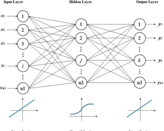
In this study, a feed-forward neural network is used in combination with an error backpropagation training algorithm, namely, the BP neural network. The BP neural network consists of one input layer, one or more hidden layers and one output layer (Fig. 1). The important issues in the establishment of topological structure include the de-termination of the number of hidden layers, the number of hidden neurons (nodes) and the transfer function. The Kolmogorov theorem has certified that a single hidden layer is competent for ANN to ap-proximate any complicated nonlinear function and establish a non-linear mapping between the input and output layers. Therefore, this study establishes a three-layer BP neural network; the topological configuration and the selection of the activation function are illustrated
inFig. 1. In contrast to the signal, the error is backward propagated, and in the process of backward propagation, the weights and deviations of the network are gradually adjusted to complete the training. The interested readers are referred toThirumalaiah and Deo, 1998, Jain and Srinivasulu, 2004, Fernando and Shamseldin, 2009, Senthil kumar et al., 2012for further details.
2.2. Svr
The basic concept of SVR is to nonlinearly map the initial data in a higher dimensional feature space and to solve the linear regression problem in the feature space (Fig. 2). Therefore, SVR usually needs to build a suitable function f(x) to describe the nonlinear relationship between featurexiand target valueyi, as shown in the following Eq.(4):
= φ +
f(x )i w· (x )i b 1
wherewis the coefficient vector,φ(xi) is the transformation function, andwandbrepresent the weight and bias, respectively.wandbare estimated by minimizing the so-called regularized risk function, as shown in the following Eq.(5):
∑
= + = R(w) 1 w C L 2‖ ‖ (y ,f(x )) 2 i 1 n ε i i 2 where 1‖ ‖w 22 is the regularization term; Cis the penalty coefficient; Lε(y ,f(x ))i i is the ε-insensitive loss function, which is calculated ac-cording to Eq.(6):
= −
Lε(y , f(x ))i i max{0, |y f(x )| - }i i ε 3
whereεdenotes the permitted error threshold, so thatεwill be ignored if the predicted value is within the threshold; otherwise, the loss equals a value greater thanε.
To solve the optimization boundary, two slack factorsξ+andξ−are
introduced:
∑
= + − + = − + ξ ξ w C ξ ξ minf(w, , ) 1 2‖ ‖ ( , ) i n 2 1 4 Subject to ⎧ ⎨ ⎩ − − ≤ + ≥ + − ≤ + ≥ − − + + y φ b ε ξ ξ φ b y ε ξ ξ [w· (x )] , 0 [w· (x )] , 0 i i i i 5The key is to develop a Lagrangian function according to the ob-jective function and the corresponding constraint conditions.
∑ ∑
∑
∑
∂ ∂ = − ∂ −∂ ∂ −∂ + ∂ −∂ − ∂ + ∂ − + = = − + − + = − + = − + H y ε y max ( , ) 1 2 ( )( )K(x , x ) ( ) ( ) i i n j n i j i n i i i n i i i 1 1 i j i j 1 i 1 i 6 Subject to∑
∂ −∂ = ∂ ∂ ∈ = − + − + ( ) 0, , [0, C] i n i i 1 i i 7 Hence, the regression function is as follows:∑
= ∂ −∂ + = − + f x( ) ( )K(x , x ) b i n i i 1 i j 8 whereK(xi,xj) is the kernel function. In this study, the simulation effect of kernel function is tested, include the Linear, Polynomial, Radial Basis Function (RBF), and Sigmoid kernels, as shown in the following equa-tion: ⎧ ⎨ ⎪ ⎩ ⎪ = = + = − = + kernel K kernel K γ b BasisFunctionkernel K kernel K γ Linear : (x,x ) x·x Polynomial : (x,x ) ( (x·x ) ) Radial : (x,x ) exp( ) Sigmoid : (x,x ) tanh( (x·x ) v) i d σ i i i i ‖x - x ‖ 2 i i i 2 9 wheredis the degree of the polynomial term,vrepresents the residuals, andγis the structural parameter in the polynomial,RBFand sigmoid kernels. Differentd,γ, and penalty coefficientCvalues will be tested in the paper.2.3. Lstm
Long short-term memory is a complex recurrent model developed byHochreiter and Schmidhuber (1997)to address the deficiencies of RNNs. In contrast to RNNs, LSTMs apply memory blocks to replace the hidden layer of RNNs. In this paper, the LSTM network consists of parallel memory blocks recurrently connected to each other, lying be-tween an input layer and an output layer, and the conceptual illustra-tion is shown inFig. 3. The LSTM block was obtained fromGers et al. (2000), and it consists of an input gate, a memory cell, a forget gate, and an output gate, as shown in Fig. 4. The corresponding forward propagation equations are presented below. For our LSTM, thefirst step is to decide what information to remove from the cell state by the forget gate. The forget gate is essentially a sigmoid function. The forget gate will generate anftvalue between 0 and 1, based on the previous mo-ment output ht−1 and current input xt to decide whether to let the
information Ct−1 that is produced in the previous moment pass or
partially pass, which is depicted by Eq.(13):
= + +
ft σ(w xxf t w hhf t - 1 b )f 10
The next step is to decide what new information will be stored in the cell state. The step is divided into two parts:first, the input gate de-termines which values will be updated. Second, the memory cell gen-erates a vector of new candidate valuesCt, which can be added to the cell state. In the next step, we combine Eqs.(14) and (15)to update the state:
=σ + +
it (w xxi t w hhi t - 1 b )i 11
= − + + − +
Ct f Ct· t 1 i tanh w xt· ( xc t w hhc t 1 bc) 12 Finally, we decide what information we are going to output. First, we decide what parts of the cell state to output by running a sigmoid layer. Then, we resize theCtvalue to -1 to 1 throughtanhand multiply
it by the output of the sigmoid gate so that we output only the target information.
= + +
ot σ(w xxo t w hho t - 1 b )o 13
=
ht ot·tanh(C )t 14
In Eqs.(13)–(17),f,i,C,oandhare the forget gate, input gate, cell, output gate and hidden output, respectively. Wx and Wh in Eqs. (15)–(17)are the input and hidden weights for the gates or cells with the corresponding subscripts;bin Eqs.(15)–(17)represents learnable biases for the gates; and σ and tanh represent the gate activation function (the logistic sigmoid in this paper) and the hyperbolic tangent activation function, respectively.
In this study, we establish a three-layer LSTM network that consists of one input layer, one LSTM hidden layer and one output layer, and we train the network with an algorithm termed backpropagation through time (BPTT), which has a similar principle to the BP algorithm, by using a backpropagation network to continuously adjust the weights and thresholds (Werbos, 1990).
3. Data and processing
3.1. Case reservoir and operation data
The Gezhouba (GZB) dam is thefirst dam across Yangtze River which built after the founding of New China (Fig. 5). It located in Yi-chang city of Hubei province, approximately 38 km downstream of the Three Gorges dam, plays a role in power generation, flood control, navigation, andfisheries, and provides other comprehensive benefits. GZB is a large-scale water project that controls a drainage area of 1 × 10⁶m2, accounting for more than half of the Yangtze River basin.
The mean annual discharge of this reservoir is 14,300 m3/s, the design-flood discharge is 86,000 m3/s, the normal water level is 66.0 m, the
maximum dam height is 53.8 m, and the total storage is 15.8 × 10⁸m3.
GZB reservoir has relatively mature operating rules, and complete, detail and long sequence operation records. These records cover all kinds of operating scenarios, such as theflood control, drought relief, peaking generation, navigation andfish spawning stimulation etc., and Fig. 2.SVR schematic diagram.
provide a large number of operating data for machine learning in this study. The reservoir hydrological data and operation data were ob-tained from the official website of China Three Gorges Corporation (http://www.ctg.com.cn/). The GZB data span a period of more than 30 years, from 1982 to 2015. The data include the inflow and outflow of the reservoir and the water level upstream and downstream of the dam measured every six hours (or four hours, when the flood peak passes through the reservoir, all reservoir operating indicators are more in-tensive monitored). These data were aggregated into daily and monthly time scales.
3.2. Model building and inputs
In this study, we use selected artificial intelligence and data mining tools, namely, the BP neural network, SVR and LSTM, to simulate the GZB reservoir operation at monthly, daily, and hourly scales. The hourly data refer to the reservoir operation data collected every two or four hours. GZB reservoir operation data span the period from 27 June
1981 to 7 September 2015. Based on the commonly accepted“80/20” split rule, the data from 1 January 2008 to 7 September 2015 are used as the test period and the remainder are used for training, as shown in Table 2. The reservoir operation data are imported as model input (decision variables) and output (target variable). Specifically, the inputs include current and previous inflow (1-moment lag), previous outflow (1-moment lag), the current and previous water level in front of the dam (1-moment lag), the current and previous water level of the downstream region (1-moment lag), and the current time (month of year). Therefore, 9 inputs are included in the model. The model output is the current outflow of the reservoir. To match the consistency of the model, all source data were normalized in the range 0.0–1.0 and were then transformed to original values after the simulation using, the normalized equation is as follows:
= − − X X X X X ori min max min 15
whereXis the normalized value;Xoriis the original value; andXminand Fig. 3.The illustration of a LSTM network with one hidden layer. (a) Folded computa-tional diagram, where the blue square in-dicates a delay of 1 time step. (b) Unfolded computational diagram, where each node is associated with one particular time instance. (For interpretation of the references to colour in thisfigure legend, the reader is referred to the web version of this article.)
Fig. 4.The conceptual illustration of the LSTM memory block. Thef, andσhrepresent the activation functions used for different gates.σfrepresent the“sigmoid” activation functionσgandσhboth represent the“tanh”activation function in this study.
Fig. 5.The location of Gezhouba (GZB) Reservoir.
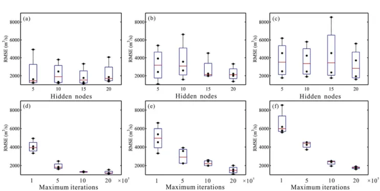
Fig. 6.BP neural network performance varies with the number of hidden nodes and maximum iterations. (a) and (d) represent the monthly statistical results; (b) and (e) represent the daily statistical results; (c) and (f) represent the hourly statistical results.
Xmaxare the respective minimum and maximum original values. The input construction was standardized for all methods, i.e., BP, SVR, and the LSTM model, to ensure an impartial comparison.
3.3. Parameterization and setting
To illustrate the strengths and weaknesses of the different AI methods, different parameterizations are used for BP, SVR and LSTM. In BP, four maximum iteration (MI) numbers are tested, i.e., 1 × 10⁵, 5 × 10⁵, 1 × 10⁶, and 2 × 10⁶, in combination with different numbers of hidden nodes, i.e., 5, 10, 15, and 20. In SVR, four types of kernel functions are set, i.e., linear, RBF, polynomial, and sigmoid kernel functions with different penalty coefficients (C, 20 values are selected from 0.0001 to 10,000, according to the geometric progression), gamma (γ, 20 values are selected from 0.0001 to 10,000, according to the geometric progression), and degree (d, i.e., 2, 3, 4). Therefore, for linear kernel function, we test 20 set of parameterizations, for RBF and sigmoid kernel function, we test 400 set of parameterizations, and for polynomial kernel function, we test 1200 set of parameterizations. Then, a performance comparison is conducted among various types of kernel functions in combination with the optimal parameters. With respect to the LSTM model, differentMInumbers are tested, including 50, 75, 100, and 200 iterations, in combination with various numbers of hidden nodes, i.e., 10, 20, 30, 40 and 50. Specific parameter
configurations are described in the results and discussion sections. 3.4. Model evaluation statistics
To mathematically quantify the skill of the model simulations, four statistical measures are calculated: the root mean square error (RMSE), RMSE-observation standard deviation ratio (RSR), and the Nash-Sutcliffe model efficiency coefficient (NSE) (Nash and Sutcliffe, 1970). The indicesRMSEandRSRare valuable because they indicate error in the units (or squared units) of the constituent of interest, which con-tributes to result analysis, andRMSEandRSRvalues of 0 indicate a perfectfit. TheNSEis a normalized statistic that determines the relative magnitude of the residual variance compared to the measured data variance (Nash and Sutcliffe, 1970).NSEvalues range from negative infinity to 1, with 1 indicating an exact match between simulated and observed values. As suggested by previous studies, anRMSEvalue less than half the standard deviation of the observed data may be con-sidered low, and ifRSR< 0.7 and NSE > 0.5, model performance can be considered satisfactory (Singh et al., 2010; Moriasi et al., 2007; Yang et al., 2017b). The equations of the selected statistics are shown below (Eqs.(19)–(20)): = ∑= RMSE n (s - o ) n i 0 i i2 16 Fig. 7.LSTM model performance varies with the number of hidden nodes and maximum iterations. (a) and (d) represent the monthly statistical results; (b) and (e) represent the daily statistical results; (c) and (f) represent the hourly statistical results.
= = ∑ − ∑ − = = RSR RMSE STDEV s o [ ( ) ] [ (o o ) ] obs i n i i i n i 0 2 0 i2 17 = −∑ ∑ = = NSE 1 (o - s ) (o - o ) i n i n 0 i i2 0 i i 2 18 whereoi andsiare the respective observed and simulated values for outflows;os andsi are the respective average observed and simulated inflows; andnis the total number of observations. In Eq. (21),r,αandβ represent the correlation coefficient, variability and bias ratio between the simulations and observations, respectively.
To estimate the uncertainty associated with model simulations, the residuals of testing sets are computed and analyzed. The analysis con-sists of three components: independence analysis, heteroscedastic analysis, and normality analysis; the implementation methods consist of plotting graphs of residual autocorrelation, residual variation relative to observed values, and residual probability distributions (Figs. 11–13).
The residual independent analysis is based on residual autocorrelation: if the residual sequence is autocorrelated, then the model fails to fully explain the variation rule of the variable, and there is some regularity that is not explained, which eventually leads to a larger prediction deviation of the model. On the other hand, low residual hetero-scedasticity and a close approximation to the normal distribution in-dicate the model is closer to unbiased estimation and has low un-certainty.
The so-called residual is the difference between the predicted value and the actual observed value, which is calculated according to Eq. (22):
=
ei oi-si 19
whereeirepresents residuals,oirepresents observed values, andsi re-presents predicted values. In this paper, the model residuals were standardized before the residual analysis, and the process is as follows: Fig. 9.Comparison of predicted and observed daily outflow using BP neural network (a), SVR (b), and LSTM (c) model.
=
r e
σ
s i, i 20
wherersrepresents standardized residuals, andσrepresents the stan-dard deviation.
All the experiments presented in this study were performed on an Inter(R) Xeon(R) CPU E5-2660 v3 @ 2.60 GHz with 64 GB DDR3 1600 MHz memory.
4. Results
4.1. Comparison of simulation results for different time scales
In this section, the observed GZB reservoir outflows are compared with simulated results based on the three different AI models, i.e., the BP neural network, SVR, and LSTM model, combined with various model parameters. First, our results show that, BP neural network and LSTM, the number of hidden nodes and maximum iterations are two key parameters that affect the simulation accuracy. Moreover, there is no obvious regularity about the effect of the number of hidden nodes on simulation accuracy, but the increase of the number of maximum iterations can significantly improve the simulation accuracy of the two models (Figs. 6 and 7). With respect to SVR, the choice of kernel function can directly affect the model accuracy. Our results show that, at monthly scale, the simulation accuracy is ranked as Sigmoid > Polynomial > RBF > Linear among the different kernel functions, at daily scale, the best accuracy ranking is Sigmoid > RBF > Linear > Polynomial; and at hourly scale, the best accuracy ranking is Sig-moid > RBF > Polynomial > Linear (Table 4).
Fig. 10.Comparison of predicted and observed hourly outflow using BP neural network (a), SVR (b), and LSTM (c) model. Table 2
The data sets sizes of training and testing the model.
Training set Testing set Total set
Monthly scale 319 93 412
Daily scale 9989 2806 12,795 Hourly scale 90,327 24,431 114,758
On the other hand, the prediction performances of the BP neural network, SVR, and LSTM model are shown in Tables 3–5 and Figs. 8–10. The calculation results show that at the monthly scale, the bestRMSEvalues obtained by the BP neural network, SVR, and LSTM model are 1122.827, 1932.814, and 161.712; the bestRSRvalues are 0.1411, 0.2429, and 0.0203; and the best NSE values are 0.9799, 0.9404, and 0.9996, respectively (Tables 3–5). The best simulation results are shown in Fig. 8. When the best statistical results are achieved, theMIandHof the BP neural network are 2 × 10⁶and 15,
respectively; the kernel function of SVR is sigmoid, the respective va-lues ofγandCare 0.1265 and 3.728; and theMIandHof the LSTM model are 200 and 50, respectively (Tables 3–5). According to the comparison among different models, the best accuracy ranking is the
LSTM model > BP neural network > SVR.
With respect to the daily time scale, the bestRMSEvalues generated using the BP neural network, SVR, and LSTM model are 1073.402, 1332.720, and 663.723; the bestRSRvalues are 0.1253, 0.1556, and 0.0230; and the bestNSEvalues are 0.9843, 0.9758, and 0.9935, re-spectively (Tables 3–5). The best simulation results are shown inFig. 9. When the best statistical results are obtained, theMIandHof the BP neural network are 2 × 10⁶and 5, respectively (Table 3), the kernel
function of SVR is sigmoid, and the values ofγandCare 0.0869 and 2.560, respectively (Table 4). In addition, theMIandHof the LSTM model are 200 and 20, respectively (Table 5). According to our ex-perimental results, the best accuracy ranking is the LSTM model > BP neural network > SVR (Tables 3–5,Fig. 9).
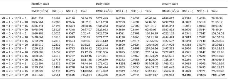
MI = 1 × 10H = 15 3335.441 0.4193 0.8224 00:38:16 4524.253 0.5282 0.7209 59:19:19 8535.343 1.0081 0.0163 80:03:27 MI = 1 × 10⁵H = 20 4075.991 0.5123 0.7348 00:37:07 3323.053 0.3880 0.8494 62:49:06 5587.853 0.6600 0.5644 75:49:24 MI = 5 × 10⁵H = 5 1610.882 0.2025 0.9587 6:20:47 3923.759 0.4581 0.7901 130:16:19 4522.122 0.5341 0.7147 158:58:52 MI = 5 × 10⁵H = 10 2478.664 0.3116 0.9019 6:35:29 3571.767 0.4170 0.8260 150:21:40 4244.474 0.5013 0.7487 160:57:31 MI = 5 × 10⁵H = 15 1762.991 0.2216 0.9504 6:36:39 2243.612 0.2619 0.9314 121:26:55 4527.507 0.5348 0.7140 162:58:32 MI = 5 × 10⁵H = 20 1855.010 0.2332 0.9451 6:35:25 2227.102 0.2600 0.9324 129:48:06 3714.903 0.4388 0.8074 159:08:51 MI = 1 × 10⁶H = 5 1269.123 0.1595 0.9743 15:34:42 2424.844 0.2831 0.9198 259:26:56 2497.333 0.2950 0.9130 334:13:15 MI = 1 × 10⁶H = 10 1319.689 0.1659 0.9722 15:17:25 2590.966 0.3025 0.9085 257:34:26 2472.812 0.2921 0.9147 386:25:26 MI = 1 × 10⁶H = 15 1283.529 0.1613 0.9737 15:12:46 1973.271 0.2304 0.9469 231:23:29 2364.631 0.2793 0.9220 397:42:26 MI = 1 × 10⁶H = 20 1366.860 0.1718 0.9702 15:11:55 1997.889 0.2333 0.9456 244:26:09 1938.357 0.2289 0.9476 357:05:48 MI = 2 × 10⁶H = 5 1202.594 0.1512 0.9769 74:44:14 1073.402 0.1253 0.9843 519:31:23 1765.321 0.2085 0.9565 799:25:59 MI = 2 × 10⁶H = 10 1179.157 0.1482 0.9778 74:30:39 1587.474 0.1853 0.9656 526:59:02 1901.642 0.2246 0.9495 805:22:17 MI = 2 × 10⁶H = 15 1122.827 0.1411 0.9799 74:05:56 2012.372 0.2349 0.9448 533:44:21 1752.630 0.2070 0.9571 792:02:28 MI = 2 × 10⁶H = 20 1551.823 0.1951 0.9616 74:22:54 1369.356 0.1599 0.9744 503:44:17 1596.052 0.1885 0.9645 786:13:09
Fig. 11.Investigation of residuals of BP neural network (Column1), SVR (Column2), and LSTM (Column3) model at monthly scale. (a–c) Autocorrelation function (ACF) plots ofrsat with 95% significance levels. (d–f)rsas a function of observed reservoir outflows. (g–i) Fitted (solid line) and actual (bars) probability density
Fig. 12.Investigation of residuals of BP neural network (Column1), SVR (Column2), and LSTM (Column3) model at daily scale. (a–c) Autocorrelation function (ACF) plots ofrsat with 95% significance levels. (d–f)rsas a function of observed reservoir outflows. (g–i) Fitted (solid line) and actual (bars) probability density function
(PDF) ofrs.
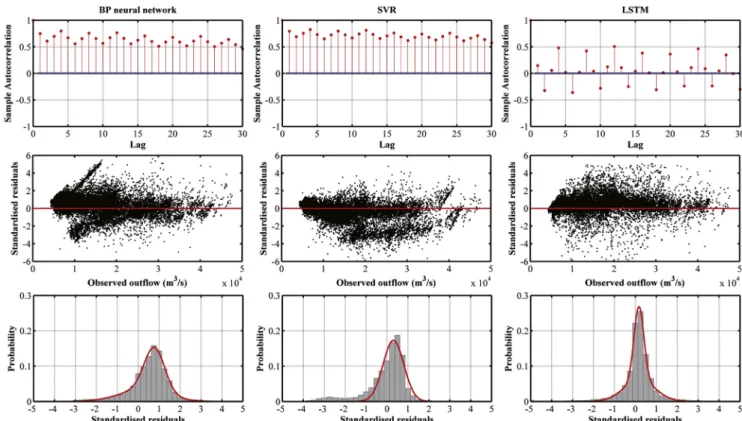
Fig. 13.Investigation of residuals of BP neural network (Column1), SVR (Column2), and LSTM (Column3) at hourly scale. (a–c) Autocorrelation function (ACF) plots ofrsat with 95% significance levels. (d–f)rsas a function of observed reservoir outflows. (g–i) Fitted (solid line) and actual (bars) probability density function (PDF)
The results of the hourly time scale suggest that the best RMSE values produced by the BP neural network, SVR, and LSTM model are 1596.052, 1051.484, and 488.121; the best RSRvalues are 0.1885, 0.1242, and 0.0577; and the bestNSEvalues are 0.9645, 0.9846, and 0.9967, respectively (Tables 3–5). The best simulation results are shown inFig. 10. When the best statistical results are achieved, theMI and H of the BP neural network are 2 × 10⁶ and 20, respectively (Table 3); the kernel function of SVR is sigmoid, the values ofγandC are 0.0464 and 2.783, respectively (Table 4), and theMIandHof the LSTM model are 75 and 50, respectively (Table 5). Notably, within a day, Gezhouba peak-load-dispatching operation according to the inflow conditions and peak frequency modulation to meet the demand of the power grid and to stabilize theflow regime of the reservoir. Therefore, compared with the monthly and daily scales, the hourly model needs to consider the predicted accuracy of outflow for the peak operation period.Fig. 10shows that the simulation accuracy of the LSTM model is higher than that of the BP neural network and SVR during the peak-load-dispatching operation period. Overall, the best accuracy ranking is the LSTM model > SVR > BP neural network.
In addition to the simulation accuracy, the calculation speed is also an important index to measure the performance of a model. In this paper, the time consumption is used as an evaluation index to compare the calculation speed of the three models. The experimental results
show that there are significant differences in the calculation speed among the three models and the three time scales. In general, the time consumption is ranked as the BP neural network > SVR > LSTM model among the different models and as the hourly scale > daily scale > monthly scale among the different time scales. The BP neural network is the longest-running model, and the time consumption in-creases asMIincreases (Table 3). The time consumption associated with optimal results at the monthly, daily, and hourly scales is 74:05′56″, 519:31′23″and 786:13′09″, respectively (Table 3). In addition to the time scale, the time consumption of SVR is also related to the selected kernel function, and the time consumption is ranked as poly-nomial > sigmoid > RBF > linear. The time consumption associated with optimal results at the monthly, daily, and hourly scales is 5′47″, 49:26′03″ and 204:16′42″, respectively (Table 4). Similar to the BP neural network, the time consumption of the LSTM model is related to the time scale and MI, which manifests as an increase in the time consumption with an increase inMI,and the time consumption asso-ciated with optimal statistical results for the LSTM algorithm is 6″, 37′04″, and 1:5′21″for the monthly, daily, and hourly scales, respec-tively.Table 5). It should be noted that the time consumption of the LSTM model is significantly lower than that of the BP neural network and SVR (Tables 3–5). Daily scale RBF γ= 0.0001C= 1438.4499 3322.261 0.3879 0.8495 45:29:31 Sigmoid γ= 0.0886C= 1.6237 1332.720 0.1556 0.9758 49:26:03 Polynomial d= 3γ= 0.0886C= 78.4760 3480.387 0.4063 0.8348 152:06:59 Linear C= 0.2336 3371.827 0.3937 0.8499 6:01:07 Hourly scale RBF γ= 0.0001C= 1438.4499 1104.779 0.1305 0.9830 163:09:45 Sigmoid γ= 0.03360C= 4.2813 1051.484 0.1242 0.9846 204:16:42 Polynomial d= 3γ= 0.6158C= 78.4760 1652.226 0.1951 0.9614 635:15:19 Linear C= 0.6158 1774.222 0.2096 0.9560 12:26:14 Table 5
Statistical performance on different time scales of LSTM with different maximum iteration (MI) and different numbers of hidden nodes (H). The bold and underlined values indicate the best statistics at same time scales.
Monthly scale Daily scale Hourly scale
RMSE(m3/s) RSR(−) NSE(−) Time RMSE-D(m3/s) RSR(−) NSE(−) Time RMSE(m3/s) RSR(−) NSE(−) Time
MI = 50H = 10 385.096 0.0484 0.9976 00:00:24 440.376 0.0514 0.9974 00:10:04 576.407 0.0681 0.9954 0:33:25 MI = 50H = 20 334.178 0.0420 0.9982 00:00:24 252.441 0.0295 0.9991 00:10:18 494.814 0.0584 0.9966 0:39:05 MI = 50H = 30 474.592 0.0597 0.9964 00:00:24 383.048 0.0447 0.9980 00:10:24 488.872 0.0577 0.9967 0:35:27 MI = 50H = 40 210.880 0.0265 0.9993 00:00:25 443.702 0.0518 0.9973 00:10:17 599.306 0.0708 0.9950 0:36:22 MI = 50H = 50 370.906 0.0466 0.9978 00:00:24 569.247 0.0665 0.9956 00:10:47 599.306 0.0708 0.9950 0:36:22 MI = 75H = 10 417.693 0.0525 0.9972 00:00:35 228.924 0.0267 0.9993 00:13:05 793.922 0.0938 0.9912 1:04:33 MI = 75H = 20 403.289 0.0507 0.9974 00:00:35 474.111 0.0554 0.9969 00:13:09 524.723 0.0620 0.9962 1:06:53 MI = 75H = 30 608.502 0.0765 0.9941 00:00:36 312.815 0.0365 0.9987 00:13:14 625.140 0.0738 0.9945 1:03:48 MI = 75H = 40 427.246 0.0537 0.9971 00:00:37 270.263 0.0316 0.9990 00:13:20 525.245 0.0620 0.9955 1:03:48 MI = 75H = 50 487.979 0.0613 0.9962 00:00:36 380.130 0.0444 0.9980 00:13:25 488.121 0.0577 0.9967 1:05:21 MI = 100H = 10 394.358 0.0496 0.9975 00:00:48 319.959 0.0374 0.9986 00:18:33 647.549 0.0765 0.9941 1:39:12 MI = 100H = 20 483.471 0.0608 0.9963 00:00:49 227.077 0.0265 0.9993 00:19:04 646.599 0.0764 0.9942 1:33:48 MI = 100H = 30 268.045 0.0337 0.9989 00:00:50 263.070 0.0307 0.9991 00:19:05 774.390 0.0915 0.9916 1:40:29 MI = 100H = 40 465.524 0.0585 0.9965 00:00:52 565.103 0.0660 0.9956 00:19:15 674.315 0.0796 0.9936 1:40:39 MI = 100H = 50 312.662 0.0393 0.9984 00:00:51 337.258 0.0394 0.9984 00:19:17 552.746 0.0653 0.9957 1:41:00 MI = 200H = 10 170.775 0.0215 0.9995 00:01:51 328.510 0.0384 0.9985 00:36:33 612.316 0.0723 0.9948 3:18:27 MI = 200H = 20 207.015 0.0260 0.9993 00:01:47 196.697 0.0230 0.9995 00:37:04 587.953 0.0694 0.9952 3:17:21 MI = 200H = 30 371.593 0.0467 0.9978 00:01:49 206.057 0.0241 0.9994 00:35:05 534.235 0.0631 0.9960 3:13:45 MI = 200H = 40 221.356 0.0278 0.9992 00:01:55 221.957 0.0259 0.9993 00:36:05 751.348 0.0887 0.9920 3:14:29 MI = 200H = 50 161.712 0.0203 0.9996 00:01:56 458.931 0.0536 0.9971 00:36:17 764.212 0.0903 0.9919 3:15:12
4.2. Residuals analysis
As shown inFigs. 11–13, to evaluate the uncertainty of the models, residual analysis is performed on the best statistical results of the three models at different time scales. At the monthly scale, the experimental results show that the rs of the SVR model has a significant
auto-correlation, and the ACF presents a trend of alternating positive and negative variations as the lag changes (Fig. 11b). Compared with SVR, the autocorrelation ofrsfor the BP neural network and LSTM model is
weak, and the ACF lies mainly in the 95% confidence interval (Fig. 11a–c). Fig. 9d–f show the scatter points ofrsas a function of
observed reservoir outflows. It is clear that thersvalues do not appear
to be randomly distributed over theflow interval for each model, and thersof the LSTM model shows an obvious increasing trend with an
increase in outflow. Fig. 11g–i display the probability density dis-tribution of rsfor the three models. The results show that the
prob-ability density distribution curve ofrsfor the BP neural network isflat
with obvious skewness, and the values ofrsare mainly distributed
be-tween−1 and 3 (Fig. 11g). With respect to the SVR model, the prob-ability density ofrsshows a bimodal distribution, ranging mainly
be-tween −2 and 0 (Fig. 11h). Thers of the LSTM model presents a
unimodal distribution with a sharp peak, and thersvalues are mainly
distributed between−2 and 2 (Fig. 11i).
At the daily scale, the autocorrelation ofrsfor the LSTM model is the
weakest, whereas thersvalues of the BP neural network and SVR model
show remarkable autocorrelation (Fig. 12a–c). Thersvalues of the three
models exhibit heteroscedasticity as the observed outflow changes. Compared with the BP neural network and SVR, the spatial distribution ofrswith observed outflow for the LSTM model is relatively uniform
(Fig. 12d–f). The probability density ofrsfor the BP neural network
displays a unimodal distribution, ranging mainly between −1 and 1 (Fig. 12g). Thersof SVR has a multimodal distribution, with three
peaks (two high and one low) distributed at−1.2, 0 and 1.4, respec-tively (Fig. 12h). The rsof the LSTM model presents a unimodal
dis-tribution with a sharp peak, andrsis mainly distributed between−1
and 2 (Fig. 12i).
The experimental results show that at the hourly scale, auto-correlation of rs is found in all three models (Fig. 13a–c). The ACF
values of the BP neural network and SVR are positive, with periodic increases or decreases as the lag changes (Fig. 13a and b). The ACF values of the LSTM model present a trend of alternating positive and negative variations as the lag changes and also exhibit the phenomenon of periodic increases or decreases. The rsvalues of all three models
exhibit heteroscedasticity (Fig. 13d–f). The probability density curve of rsfor the BP neural network model has a single peak, ranging mainly
between−1 and 2, and obvious (mainly positive) skewness is exhibited (Fig. 13g). The distribution ofrsfor the SVR model is also unimodal,
and a wide distribution is evident between−4 and 2 (Fig. 13h). With respect to the LSTM model, the probability density curve ofrsis
un-imodal, and rs is densely distributed, mainly between −1 and 1
(Fig. 13i).
4.3. Comparison of simulation results for differentflow regimes
The experimental results of Section 4.2 show that model uncertainty varies with observedflow. To better determine the ability of the models to reproduce differentflow regimes, the models with the best simula-tion results are evaluated for three specific regimes, i.e., low, inter-mediate and highflow conditions. The division of theseflow regimes is based on the calculation of the inflow frequency distribution curve. The flow regimes are categorized by using the 25th and 75th percentiles, and the flow limit is 5985 m3/s and 18,050 m3/s, respectively. The
model accuracy for the differentflow regimes is graphically represented in three scatter plots (Figs. 14–16) and is measured in terms ofRMSE, RSR, andNSE(Table 6). The experimental results show that, in general, the LSTM model has a significant advantage with respect to simulation
accuracy, and this model can produce more accurate simulation results for each time scale andflow regime. Specifically, at the monthly scale, the comparison results show that the evaluation index values of the LSTM model are the best and the simulation accuracy is the highest; the comparison results of the two other models show that, under lowflow conditions, the simulation accuracy of these two models is not ideal, i.e., theRSRvalue is greater than 1, and theNSE value is negative. Under intermediate and highflow conditions, the simulation accuracy of the two latter models meets the evaluation criteria, and the accuracy of the BP neural network simulation is higher than that of SVR (Table 6, Fig. 14). At the daily time scale, the simulation accuracy of the LSTM model is significantly higher than that of the two other models. Under low flow conditions, poor simulation is observed for the BP neural network and SVR, and it is difficult to obtain satisfactory results. Under intermediate and high flow conditions, both of these models exhibit satisfactory simulation results; the simulation accuracy of the SVR model is slightly higher than that of the BP neural network under in-termediateflow conditions, whereas the simulation accuracy of the BP neural network is higher than that of SVR under highflow conditions (Table 6, Fig. 15). At the hourly scale, the LSTM model also shows higher prediction accuracy than the BP neural network and SVR (Table 6). The simulation accuracy of the BP neural network and SVR is poor under low flow conditions. Under intermediate and high flow conditions, the simulation accuracy of the two models meets the eva-luation criteria; the simulation accuracy of SVR is higher than that of the BP neural network under intermediateflow conditions, whereas the simulation accuracy of the BP neural network is slightly higher than that of SVR under highflow conditions (Table 6,Fig. 16).
5. Discussion
5.1. Suggestions for model parameterization
Parameter setting has always been the focus of the performance research of AI models. In this study, we test the influence of different parameter combinations on the performance of three selected AI models. First, we explore the effect of the maximum number of itera-tions and the number of hidden nodes on the accuracy of a BP neural network. According to the statistics shown inTable 3for the BP neural network, (1) in general, an increase in the number of maximum itera-tions can improve the simulation accuracy, and (2) the effects of the number of hidden nodes on the simulation accuracy are uncertain and irregular. In addition, selection of the appropriate number of hidden nodes can help improve the statistics. As shown inTable 3, the best BP neural network statistics for the three time scales are consistently achieved by a maximum number of iterations equal to 2 × 10⁶. In the
use of the BP neural network in our study, an error backpropagation combined with a gradient descent algorithm is employed. As the number of maximum iterations increases, the gradient optimization scheme continuously explores the response surface of the objective function (Eq.(3)), and the evolution is not completed until the algo-rithm reaches the preset error value or the allowable number of max-imum iterations. However, as the search evolves with more iterations, the gradient of the objective function will decrease; consequently, any further increase in the maximum iteration number results in less im-provement in the objective function value, as shown for the 1 × 10⁶ and 2 × 10⁶maximum iteration scenarios in Table 3. In addition, to ensure that the network training reaches the maximum number of iterations, the error value is set as 0.0001, which is significantly lower than that of the model. Our results show that choosing the appropriate number of hidden nodes can significantly improve model accuracy, but the effect of the number of hidden nodes on accuracy is unpredictable. The best BP neural network statistics for the monthly, daily, and hourly time scales are obtained when the number of hidden nodes is 15, 5, and 20, respectively (Table 3). As mentioned inYao (1999), the number of hidden nodes in ANN is crucial for model performance and should be
jointly designed and optimized with a proper training algorithm. As such, the number of hidden nodes is one of the research hotspots in the ANNfield. It is generally believed that determination of the number of hidden nodes is related to the number of input and output nodes (Lippmann, 1987; Chen, 1996; Moody and Antsaklis, 1996). Never-theless, studies have not adopted a universally accepted method for choosing the number of hidden nodes. At present, the number of hidden nodes is usually determined by trial and error with the objective of minimizing the cost function.
With respect to SVR, we examine the influence of the kernel func-tion on the simulafunc-tion performance based on an optimal structural parameter (γ), penalty coefficients (C) and degree (d, for the poly-nomial). The kernel function is introduced to map the linear non-separable training sample from the input space to the feature space, thereby realizing the linear separability of the training samples in the feature space. In this way, a linear classifier can be used to divide the training samples after mapping in the feature space. As shown in Table 4, SVR models are able to produce satisfactory results, but the simulation accuracy and time consumption differ significantly among different kernel functions. Our results show that, regardless of the time scale, the best simulation accuracy is consistently generated by the sigmoid kernel function; however, the time consumption of this func-tion is relatively long (Table 4). This is not consistent with previous research, and most reviewed studies have suggested that RBF is the most appropriate kernel function that tends to exhibit satisfactory performance (Yaseen et al., 2015). However, technological research conducted on the kernel function shows that any kernel function has its own advantages and limitations because of different training samples, and kernel functions have different classification abilities (Amari and Wu, 1999; Asefa et al., 2006; Yang et al., 2017b). The sigmoid kernel function is derived from ANN and has been proved to have good global classification performance (Lin and Lin, 2005). Our results also show that the classification performance of the sigmoid kernel function is better than that of other kernel functions for our training sample.
With respect to the LSTM model, we mainly consider the influence of the number of maximum iterations and hidden nodes on model performance, and the main results in this paper are as follows: (1) an increase in the number of maximum iterations improves the precision of the LSTM model, and (2) a change in the number of hidden nodes affects the simulation accuracy, but the function is weak and irregular.
As shown inTable 5, when the number of maximum iterations increases from 50 to 75, the model accuracy is effectively increased, but in-creasing the number of maximum iterations to greater than 100 does not improve accuracy further. Based on an advanced investigation, we deduce that model accuracy is not improved further because the training process of the LSTM model adopts the BPTT algorithm, which has a similar principle as the classical BP algorithm. The BPTT algo-rithm uses a forward algoalgo-rithm to calculate the output value, backward calculates the error of each individual LSTM cell, and continuously updates the network weight, extending the direction to reduce the error. With the narrowing of the gap between the model’s output value and the desired output value, the decline rate of the model error tends to slow down, so an increase in the number of maximum iterations does not significantly improve model precision when the number of max-imum iterations reaches a certain limit. However, unlike the BP neural network, the number of iterations required for LSTM model con-vergence is much smaller than the BP neural network. Our analysis indicates that the reason for this result is that the LSTM model has strong feature extraction capabilities, which ensures that the model can extract the characteristic information of the data more efficiently and complete the convergence process quickly. According to our experi-mental results, we cannot specify how to achieve the best statistics by choosing the number of hidden nodes. However, it is worth noting that while the number of iterations is the same, the changes of number of hidden node have only a limited effect on the simulation accuracy. At present, studies that examine the influence of the number of hidden nodes on the precision of LSTM models are rarely reported.Wielgosz et al. (2017)tested the influence of the number of hidden nodes on simulation accuracy and concluded that, for their test data, the simu-lation accuracy was highest when the number of hidden nodes was 32, but the effect of different numbers of hidden nodes on model accuracy was not discussed in detail.
In conclusion, we believe that priority should be given to the number of maximum iterations in the BP neural network and LSTM model building, and a reasonable increase the number of maximum iterations can significantly improve the model accuracy. In contrast, the number of hidden nodes has a weak effect on model accuracy. For the SVR model, the selection of kernel function is the key to model con-struction. Combined with previous research results, we believe that sigmoid and RBF kernel function can be considered the priority object. Fig. 14.Scatter plots of predicted and observed hourly outflow for BP neural network (a), SVR (b), and LSTM (c) model. Different colors are used to represent the
flow regimes.
Fig. 15.Scatter plots of predicted and observed daily outflow for BP neural network (a), SVR (b), and LSTM (c) model. Different colors are used to represent theflow regimes.
Meanwhile, in the process of model construction, due to differences in data volume and structure, model parameters have different influences on model performance. Therefore, we suggest that the model should be repeatedly trained before practical application to determine the optimal parameters and ensure the prediction ability of the model.
5.2. Suggestions for the applicability of AI models under different scenarios The AI model has the ability to address complex nonlinear predic-tion problems, which is widely applied in thefield of reservoir opera-tion simulaopera-tion. At present, reports on the performance comparison and analysis of AI models are common, but such reports mainly focus on the global precision comparison analysis of a single time scale. However, analyzing the global and extreme event simulation performance of the model from multiple time scales is the key to the model comprehensive learning operation rule and generating long and short-term operation plans for different scenarios. Therefore, in this study, we analyzed the simulation results of the BP neural network, SVR and LSTM under different time scales andflow regimes from three aspects of model accuracy, uncertainty and calculation speed. Based on the above ana-lysis, we explored the guiding significance of three AI models for re-servoir long and short-term operation, and the coping capacity of three AI models for extreme inflow conditions such as drought andflood, and we summarized the application scenarios of each model in order to provide a reference for the practical application of these model.
First, the application effect of the BP neural network in reservoir operation was studied. In the 1990s, the emergence of BP algorithm greatly facilitated the development of ANN and effectively promoted the research of ANN algorithms in thefield of reservoir operation. In our study, the BP neural network was applied to the reservoir operation simulation, and the results showed that, for reservoir long-term op-eration (monthly scale), the simulation accuracy of the ANN model is good, the uncertainty is weak, and the time consumption is long; at the daily scale, the accuracy of the BP model still met the evaluation cri-teria, but the residuals were autocorrelated and exhibited hetero-scedasticity, and the time consumption increased. At the hourly scale,
due to the further increase in data volume, the disadvantages of the model regarding the uncertainty and time consumption are more ob-vious (Table 3). Thus, we consider that if the model is able to learn the operation rule of a reservoir from a small amount of data (such as the research of reservoir long-term operations or the influence factors of reservoir operations), the BP neural network can obtain satisfactory simulation accuracy and the time consumption is not too long, so it can be used for the simulation of reservoir operations. However, for large reservoirs and the short-termfine operation of reservoirs, the data that are required by the model learning reservoir operation rules are large, due to the large number of influencing factors. In this case, the time consumption of the BP neural network is too long, and the applicability is weak. On the other hand, for differentflow regimes, the results show that under intermediate and highflow conditions, the BP neural net-work can obtain satisfactory results, but under lowflow conditions, the BP neural network has poor simulation results and is not suitable for simulation of low inflow scenarios.
Because the feature extraction ability is poor, the training time of the BP neural network is too long, and the practical application is limited, the emergence of the SVR algorithm partly compensates for the deficiency in BP neural networks. The SVR algorithm introduces the Lagrangian method to simplify the quadratic optimization problem in SVR calculations and introduces the kernel function to reduce the complexity of high-dimensional computations, thus allowing the SVR model to calculate the high efficiency characteristics. This paperfirst compares the processing power of the model to different time scale problems. The results show that the SVR algorithm can attain sa-tisfactory statistics, but compared with the BP neural network, the two models have advantages and disadvantages. At monthly and daily time scales, the accuracy of the BP neural network model is higher than SVR, and at the hourly time scale, the calculation accuracy of the SVR model is higher than that of the BP neural network (Tables 3 and 4). In this study, the simulation ability of the model to different time scale pro-blems reflects the processing power of the model to different data vo-lumes to some extent. Therefore, the BP neural network has a stronger processing capability than SVR when the data volume is small, whereas Fig. 16.Scatter plots of predicted and observed hourly outflow for BP neural network (a), SVR (b), and LSTM (c) model. Different colors are used to represent the
flow regimes.
Table 6
Statistical performance on differentflow regimes of BP neural network, SVR, and LSTM. The bold and underlined values indicate the best statistics for eachflow regimes at same time scales.
Lowflow Intermediateflow Highflow
BP SVR LSTM BP SVR LSTM BP SVR LSTM
Monthly scale RMSE(m3/s) 920.057 578.508 75.719 1262.017 1739.038 150.391 912.0822 3101.806 243.847
RSR(−) 2.3805 1.4968 0.1959 0.3213 0.4428 0.0383 0.1768 0.6011 0.0473
NSE(−) −4.9370 −1.3472 0.9598 0.8947 0.8001 0.9985 0.9670 0.6186 0.9976 Daily scale RMSE(m3/s) 475.169 784.946 118.550 1350.407 1255.688 354.916 963.313 1897.362 179.351
RSR(−) 1.2718 2.1009 0.2850 0.3805 0.3538 0.1000 0.1509 0.2973 0.0281
NSE(−) −0.6195 −3.4194 0.9174 0.8551 0.8747 0.9900 0.9772 0.9115 0.9992 Hourly scale RMSE(m3/s) 1058.031 496.4571 102.934 1861.919 899.2275 527.392 1606.689 1711.116 478.904
RSR(−) 2.7868 1.3077 0.2710 0.5227 0.2524 0.1480 0.2584 0.2752 0.0770
flow conditions (Table 6,Figs. 14–16).
In view of the above problems, namely, that the simulated speed of the traditional AI models is slow, the accuracy needs to be increased, and it is difficult to address extreme events, we turned our attention to the LSTM model, which performed well in solving the time series problems. Taking the GZB reservoir as an example, this paper con-structs an LSTM model to predict the outflow of the GZB reservoir and explores the application of LSTM in reservoir operations. The results show that the LSTM model effectively makes up for the deficiency of the traditional AI models. Whether from the accuracy, uncertainty, calcu-lation speed, extreme conditions processing, the LSTM has significant advantages over the BP neural network and SVR (Tables 3–6, Figs. 8–16). Especially at the hourly scale, facing vast amounts of data, LSTM performance is outstanding, and the training and prediction process takes only approximately an hour. Meanwhile, LSTM is the only one of the three models that can accurately simulate the outflow curve of GZB for the peaking operation period (Fig. 10). The experimental results for show that the LSTM model overcomes the disadvantage of previous models, i.e., poor simulation accuracy for extreme events, and the LSTM model can accurately predict reservoir outflow under low and high inflow conditions. In conclusion, compared with the BP neural network and SVR, the LSTM model has significant advantages in terms of simulation accuracy, stability and computing speed, and we believe that LSTM, as a deep learning model, has a strong sequential predictive ability and can be used for reservoir operation simulations. At present, the application of the LSTM model in reservoir operation has been rarely reported, butZhang et al. (2018)arrived at similar conclusions in the study of sewage overflow prediction, which can provide some re-ference for us.Zhang et al. (2018)compared the predictive effects of the LSTM and SVR models on sewage discharge, and the results showed that the simulation accuracy of the LSTM model was significantly higher than that of the SVR model, which was similar to our conclusion. In summary, with respect to the AI model applicability, the BP neural network is suitable if the model is able to learn the operation rule of a reservoir from a small amount of data (such as the research of reservoir long-term operations or if the influence factors of reservoir operation are small). For large reservoirs, short-termfine operation of reservoirs and low inflow conditions, the applicability of the BP neural network is weak. The main limitation of the BP neural network is that the independent feature extraction ability of the network is poor, so the time consumption required for satisfactory results is too long. The ap-plicability of the SVR model and the BP neural network is similar. Although the SVR model improves computing speed, its ability to ad-dress massive data and low inflow conditions is still insufficient. By contrast, the LSTM model has obvious advantages and can quickly and accurately simulate the reservoir operation under various time scales andflow conditions. Therefore, LSTM can be used for medium- and long-term reservoir operation and short-term refinement operation si-mulation, as well as to address various emergencies. Meanwhile, the LSTM effectively solves the time consumption problems of the BP neural network and SVR model corrects for the fact that traditional AI cannot simulate lowflow conditions or the outflow curve for the peak operation period.
6. Conclusions
Reservoir operation is an important part of reservoir management, and the theory and method of reservoir operation have been gradually
and artificial demand, and the operation often deviates from the op-erating rules, which limits the application of such models. AI models, or data-driven models, are able to autonomously learn the operating rules from the historical operation data of a reservoir and thus have greater robustness and are good at dealing with complex factors.
This paper investigated the usefulness of two traditional AI models (BP neural network and SVR) and a new deep learning model (LSTM model) in assisting reservoir operation. Detailed discussion and re-commendation are made with respect to the process of model para-meter settings, the simulation performances, and the applications of employed AI models under different flow regimes and temporal re-solution. The main conclusions are as follows:
(1) With respect to parameter setting, our results show for the BP neural network and LSTM model, the effects of the number of maximum iterations on model performance should be prioritized. The effects of the number of hidden nodes on model performance are limited. For the SVR model, the simulation performance is di-rectly related to the selection of the kernel function. Combined with previous research results, we consider that sigmoid and RBF kernel functions should be prioritized in uses of SVR model. Meanwhile, in the process of model construction, due to differences in data volume and structure, model parameters have a different influence on model performance. Therefore, we suggest that the model should be repeatedly trained before practical application to determine the optimal parameters and ensure the prediction ability of the model. (2) With respect to the AI model applicability, the BP neural network is suitable if the model is able to learn the operation rule of a reservoir from a small amount of data (such as the research of reservoir long-term operation or if the influence factors of reservoir operation are small). For large reservoirs, short-termfine operation of reservoirs and low inflow conditions, the applicability of the BP neural net-work is weak. The main reason to limit the application of the BP neural network is that the independent feature extraction ability of the network is poor, so the time consumption required for sa-tisfactory results is long. The applicable conditions of the SVR model and BP neural network are similar. Although the SVR model improves computing speed, its ability to address massive data and low inflow conditions is still insufficient. By contrast, the LSTM model has obvious advantages and can quickly and accurately si-mulate the reservoir operation under various time scales andflow conditions. Therefore, LSTM can be used for medium- and long-term reservoir operation and short-long-term refinement operation si-mulation, as well as to address various emergencies.
(3) The LSTM model can effectively solves the time consumption pro-blem associated with the BP neural network and SVR model, and it has superior performances over other AI models in simulating re-servoir operation during low-flow conditions or the outflow curve for the peak operation period, whereas traditional BP neural net-work and SVR model tend to fail.
Acknowledgement
The data presented in this paper are available at the official website of the China Three Gorges Corporation (CDEC):http://www.ctg.com. cn/. This paper is a part of a joint cooperation between the China Institute of Water Resources and Hydropower Research and the University of California, Irvine. This work was supported by the