Report EUR 27513 EN
2 0 1 5
Contributors.
Daniele Ehrlich, Andreea Julea, Martino Pesaresi
Forename(s) Surname(s)
Global spatial and temporal analysis of human
settlements from Optical Earth Observation:
Concepts, procedures, and preliminary results
European Commission Joint Research Centre
Institute for the Protection and Security of the Citizen
Contact information Daniele Ehrlich
Address: Joint Research Centre, Via E.Fermi 2749, TP267, I-21027 Ispra (VA), Italy E-mail: [email protected]
Tel.: +39 0332 789384
JRC Science Hub https://ec.europa.eu/jrc
Legal Notice
This publication is a Technical Report by the Joint Research Centre, the European Commission’s in-house science service.
It aims to provide evidence-based scientific support to the European policy-making process. The scientific output expressed does not imply a policy position of the European Commission. Neither the European Commission nor any person acting on behalf of the Commission is responsible for the use which might be made of this publication.
All images © European Union 2015 JRC96929 EUR 27513 EN ISBN 978-92-79-52711-1 (PDF) ISBN 978-92-79-52712-8 (print) ISSN 1831-9424 (online) ISSN 1018-5593 (print) doi:10.2788/745756
Luxembourg: Publications Office of the European Union, 2015
© European Union, 2015
Reproduction is authorised provided the source is acknowledged.
Printed in Luxembourg
Abstract
This report provides an overview on the concepts, processing procedures and examples used to quantify changes in built-up land from optical satellite imagery. This is part of the larger work of the Global Human Settlement (GHS) team from the Joint Research Centre (JRC) that aims to measure the spatial extent of global human settlements, to monitor its changes over time and characterize the morphology of settlements. This built-up change analysis addresses the quantification of urbanization including some socio-economic and physical processes associated with urbanization. This includes the quantification of the building stock for modeling physical exposure in disaster risk modeling, to be used as background layer for emergency response when a disaster unfolds and as background building stock layer for normalizing physical loss data.
Based on the application of three of the most used change detection methods, Principal Component Analysis, Image Differencing Comparison, and Post-Classification Comparison, we present and discuss preliminary results, and try to identify future research directions for developing an appropriate approach for GHSL result images. The case studies were carried on Alger and Dublin city areas.
Contents
Abstract ... 4
1.
Introduction ... 4
2.
Terminology ... 5
2.1.
Scales ... 5
2.2.
Human settlements, built environment, and urban areas ... 7
2.3.
“Urban” quantitative measures ... 8
2.4.
Global Human Settlements ... 9
3.
Change detection for human settlements spatial growth study ... 12
4.
Change Detection tests ... 14
4.1.
Alger case study ... 14
4.1.1.
Methodology ... 15
4.1.2.
Results ... 16
4.1.3.
Discussion ... 17
4.2.
Dublin case study ... 18
4.2.1.
Input data and preprocessing ... 18
4.2.2.
Methodology ... 20
4.2.3.
Results ... 23
4.2.4
Discussion ... 26
5.
Conclusion ... 27
Spatio-temporal analysis of human settlements
from Optical Earth Observation
Concepts, procedures, and preliminary results
Abstract
This report provides an overview on the concepts, processing procedures and examples used to quantify changes in built-up land from optical satellite imagery. This is part of the larger work of the Global Human Settlement (GHS) team from the Joint Research Centre (JRC) that aims to measure the spatial extent of global human settlements, to monitor its changes over time and characterize the morphology of settlements. This built-up change analysis addresses the
quantification of urbanization including some socio-economic and physical processes associated with urbanization. This includes the quantification of the building stock for modeling physical exposure in disaster risk modeling, to be used as background layer for emergency response when a disaster unfolds and as background building stock layer for normalizing physical loss data.
Based on the application of three of the most used change detection methods, Principal Component Analysis, Image Differencing Comparison, and Post-Classification Comparison, we present and discuss preliminary results, and try to identify future research directions for developing an appropriate approach for GHSL result images. The case studies were carried on Alger and Dublin city areas.
1.
Introduction
In simple terms, we can define human settlements as any form of human habitation which ranges from a single dwelling to large city and megacity. Human settlements are the part of the landscape covered with man-made structures that include buildings, roads and transport networks. It is also where people are to be found for most of the time as it is where they live and perform their economic and recreational activities. In fact, settlements are studied by
demographers, economists, sociologists as well as urban planners and geographers (Seto et al. 2014). This report addresses the physical part of human settlements that relates to the
structures built by humans and spatially grouped in spatial clusters. This term is similar to that of built environment which is similarly defined. The term has also been adapted as output of image processing related to the built environment (Pesaresi & Ehrlich 2009) and used to define a range of remote sensing products (Gamba & Herold 2009).
Information on the physical part of human settlements is used to address a number of unanswered questions relevant for a number of application areas. For example, how much of the land masses is covered by villages and cities today and how much land will be used to host the settlements of tomorrow? What is the rate of growth associated to urbanization in the different regions of the world? What are the old and the new patterns of growth? There are more practical issues to address also. For example, how fast do single cities expand spatially? How do cities compare spatially in size? How does the augmentation in global built up increase the risk due to environmental hazards?
Quantitative information on human settlements is used to understand the complex interactions between human activities and global physical processes – those that are under the scrutiny of the global change scientific community. Most importantly, this work addresses the
triggered by natural events. Measuring the built environment for crisis management would serve a number of users that are operating at different scales with different information needs. The international crisis management community operates globally, but requires information that is sufficiently precise for local applications. Among the different services that may use fine scale global human settlement information, we include the Global Disaster Alert and
Coordination System (GDACS) (Global Disaster Alert and Coordination System 2015) that provides early warnings by generating automatic alerts, Copernicus Emergency Management Service (Copernicus Emergency Management Service 2015) that would benefit from pre-disasters data to access fast damage assessments for estimating the severity and extent of the disaster, the loss data initiative that would benefit from exposure information to calibrate the losses estimated over a given area to the actual assets exposed (De Groeve et al. 2014)
(De Groeve et al. 2013). This is particularly relevant when comparing and estimating losses over time in areas of rapid urbanization. This analysis would be of use to technical offices of UN emergency agencies, donor institutions, International Non-Governmental organizations that work on similar tasks and that often cooperate with the services of the Commission, and to international research programs such as Integrated Research on Disaster Risk (Integrated Research on Disaster Risk 2015).
2.
Terminology
Human settlements are addressed by a number of disciplines and each comes with its own terminology. As in many other cross cutting terminologies, the definitions in one field can bear slightly different meanings in other fields. Definitions may be used in different contexts or the same concepts may be defined differently. For example, demographers refer to urban areas as locations with high concentration of people, economists as areas with specific productive functions typically of the service sector, sociologists as people with specific ways of life (Seto et al. 2014). This work uses the term related to the built environment as used by geographers and urban planners that address the quantification of the spatial extent of settlements and its different sub components. The paragraphs below review the most common terms related to the built environment and intend to clarify the definitions for use in global human settlement analysis.
The term human settlement is often used interchangeably with urban areas (Seto et al. 2014), even if urban areas are typically associated with larger human settlements such as towns, cities and megacities. Human settlements – and this is the term used within this document - aim to include every single settlement, irrespective of their size. That is a precondition to be able to measure changes in time.
The next two sections list - and where necessary comment - the terms used for describing and quantifying the built environment and changes in time as addressed in this work. The first section presents a list of general terms that provide the narrative for describing the built environment, while the second, the more quantitative terms used to measure it; section three reviews the use of the term “urban” and the last section conceptualize the use of terms within the Global Human Settlement project.
2.1.
Scales
Human Settlements – the focus of this analysis - can be measured taking into account different “scales”. The term scales relates to the process/object under analysis: a) the type and precisions in the measurement devices, b) the geographical extents under scrutiny, c) the time intervals investigated; d) the content of the information products derived and mapped, and e) proxy variables for the processes/objects investigated. For the sake of clarity, we use the different definitions of scale proposed by Wu and Li (Wu & Li 2009), commented to accommodate the analysis of human settlements as follows:
Operational (Phenomenon) scale – the scale at which the phenomenon (human settlement) manifests itself. The operational scale refers to the size of the built up structures and settlements that are being measured as well as to their spatial
arrangement. For example, the land covered by buildings – often referred as building footprint - may range from building covering tenths of square meters – as for dwellings - to construction covering square kilometers as in the case of commercial or industrial buildings. Floors may be spaced vertically approximately 3 meters for dwellings and much higher for recreational or industrial buildings. The buildings may be one, two stories as well as 10, 20 stories high to reach the towers of the world extending hundreds of meters in height. There are many exceptions, in the spatial size, the floor height and the total height of the buildings. Overall, however, human inhabited space is relatively similar across the 5 continents and statistics can be obtained from census offices. The settlements are thus the clustering of these building structures.
Geographical scale - the spatial extent of the study/research geographical space, often also referred as coverage. This work addresses the global human settlements, the scale being the planet Earth. However, occasionally, we compare limited areas on the ground such as a city or a metropolitan area and the geographical scale is thus in the order of 200 km2 (as in this case study analysis) to 100 000 km2 to accommodate changes in
some of the largest metropolitan areas.
Observation (Measurement) scale – the measurement intervals (units) at which data is collected. Observations may be very precise (fine scale) and less precise (coarse scale). Observation scale relates to the spatial resolution of the imagery used to analyze the settlements, thus being a key point in the detection and quantification of settlements. Fine observation scale allows the detection of the smallest building and structure. Coarser scale will only allow the detection and possibly the measurement of larger settlements.
Modeling scale
–the scale at which the model is built to reproduce the
phenomenon under investigation. The modeling scale is defined by the spatial
unit used for the tessellation of space. The square cell grid is the most often used
tessellation. The density of built up computed over the grid is the model used
within the global human settlement. This model varies with changing the grid
cell size. The size of the grid used in modeling will depend also on the
measurement scale.
Cartographic scale – the ratio between the map distance (traditionally on the paper printed map) and the ground distance. Cartographic scale contains embedded also the notion of information content and is thus often used to replace the concept of modeling scale. In fact, when referring to cartographic scale, we also refer to the inherited
information content that is related to that scale. In this work, information produced at cartographic scales smaller than 1:100 000 uses original built up information
generalized through a model (modeling scale) to larger grid cells.
Time scale – the time scale at which the phenomenon is expected to show spatial changes, or the time interval with which the information is collected.
The measurement scale, a key point of this work, is the one that relates to spatial resolution. For practical purposes, we use the classification of the Copernicus service (Copernicus Space
Component Data Access Portal - Mission Groups 2015) that categorizes the imagery as in Table 1. For the sake of simplicity, we will refer to VHR for VHR-1 and 2, to HR for HR-1 and 2 and to MR for MR-1 and 2.
Table 1. Classification of optical imagery based on spatial resolution (Copernicus)
VHR-1 VHR-2 HR-1 HR-2 MR-1 MR-2 LR
Spatial
Resolution <1m 1-4m 4-10m 10-30m 30-100m 100-300m >300m
2.2.
Human settlements, built environment, and urban areas
Human settlements are places and locations where people aggregate to live. They are defined as follows: “The term human settlement is an integrative concept that comprises: (a) physical components of shelter and infrastructure; and (b) services to which the physical elements provide support, that is to say, community services such as education, health, culture, welfare, recreation and nutrition” (United Nations, Department for Economic and Social Information and Policy Analysis, Statistics Division 1997). The definition clearly subdivides the physical part – on which this work focuses on – and the more socio-economical part not addressed in this
document.
The physical description of human settlements can include everything from simple housing to entire cities. In fact, the term human settlement is also a general term that relates to a hierarchy of population concentration. The typical hierarchy (Doxiadis 1968) includes isolated dwellings, hamlets, villages, towns, large towns, cities, large cities, metropolis, conurbations, and
megalopolis/megacities. The hierarchy of settlements is based on the total population of the settlements and is used with small modification also within the UN system (United Nations, Department for Economic and Social Affairs, Population Division 2006). Within the definitions, the spatial aggregation of the settlements is implicit but not formally stated. The definition of settlement also includes the physical part including built up structures, as well as infrastructure, which is similar to the definition of the built environment.
Built environment and the physical definitions of settlements are to be found in a set of terms used by civil engineers that include the following. Built up - “covered with buildings” (Merriam-Webster, Inc. Publishers 1989); Built up area – a developed area that includes land on
which buildings structures and/or non-building structures are present. Structures are “something (like a building) that is constructed” (Merriam-Webster, Inc. Publishers 1989). Building - “A usually roofed and walled structure built for dwelling or permanent use”
(Merriam-Webster, Inc. Publishers 1989), while Non-Building structures refer to any physical body or system not designed for human occupancy. The non-building structures are also referred in civil engineering as civil works.
The term most often used in describing the built environment is that of urban area. An urban area is a location characterized by high human population density and vast human-built features in comparison to the areas surrounding it. Urban areas may be cities, towns or
conurbations. The term is not commonly used to describe villages and hamlets that are referred to as rural settlements. Urban area is thus more restrictive if compared to human settlements that include all built up areas of all sizes.
Urbanization and urban sprawl relate to changes in population size and therefore in changes in built up. Urbanization is referred by demographers as a social phenomenon that refers to the shift of population from less dense (rural) to dense built up areas (urban areas), as well as "the gradual increase in the proportion of people living in urban areas”. However, the outcome of urbanization is the physical growth of built up areas that is addressed by urban planners and also referred to as urban growth and recently as spatial growth (East Asia’s Changing Urban Landscape: Measuring a Decade of Spatial Growth 2015). This physical growth may be both horizontal and vertical, the horizontal part having direct implication with the measurement of
the extent of the built environment addressed in this document. The spatial growth is also related to the concept of urban sprawl.
Urban sprawl or suburban sprawl typically describes the expansion of human population away from central urban areas into low-density, mono-functional and usually car-dependent communities. In addition to describing a particular form of urbanization, the term also relates to the social and environmental consequences associated with this development. While sprawl is a social phenomenon, it is also accompanied by changes in the built up environment. Sprawl is often understood as a growth of the city’s built up area (Urban Sprawl in Europe, The ignored challenge 2006). The growth of built up land is being often referred to also as urban growth (Miller & Small 2003), urban expansion (Seto et al. 2014) or spatial urban growth (East Asia’s Changing Urban Landscape: Measuring a Decade of Spatial Growth 2015). It is this spatial growth (East Asia’s Changing Urban Landscape: Measuring a Decade of Spatial Growth 2015), or the spatial urban growth (Seto et al. 2014), or the “sprawl” as defined by the European
Environmental Agency (Urban Sprawl in Europe, The ignored challenge 2006), which is the focus of the analysis of changes in human settlements.
The urban and rural figures collected by national statistical offices are not well suited to
measure spatial growth or spatial urban growth. The urban/rural dichotomy ignores half of the human settlements (the rural ones) and this is not suited for the analysis of settlements that requires the quantification of all settlements. Quantifying and mapping also the smaller settlements – the rural ones - is particularly important because large part of the new spatial growth in built up land (“urban growth”/ expansion) is likely to occur around the smaller (rural) settlements.
The following section identifies the typical measures on which today’s statistics are based, its shortcomings and the proposed GHS terminology.
2.3.
“Urban” quantitative measures
The term “urban” is used by census offices that report on urbanization as well as in the remote sensing literature where urban is a class within a land cover classification scheme. This is briefly elaborated bellow.
The term urban has been adopted officially in all census globally, together with the counterpart rural. The term urban refers to high density populated places. It is used by official statistics worldwide. The inhabited areas are subdivided in urban and rural, based on one or more criteria. These criteria are defined at the national level within statistical offices. All countries however report and provide the information to the UN Department of Economic and Social Affairs that publishes the statistics in their global population reviews (United Nations, Department of Economic and Social Affairs, Population Division 2015a), i.e. UN population review. The shortcomings of the urbanization figures, as compiled and reported in UN reports (United Nations, Department of Economic and Social Affairs, Population Division 2015b) relate to the modifiable area units used by the different countries to collect the data, and to the changing criteria for defining urban and rural in each country (Satterthwaite 2010).
Urban is also the preferred term in land cover and land use classification system used within the remote sensing community that can overlap with that of human settlements. The term is not always precisely defined and is used to label information products from images at different spatial resolution. For example, few low-resolution derived global land cover products – with the exception of MODIS Land Cover product (Friedl et al. 2010) – define precisely the semantic of the urban class/classes. The continental derived information products, such as the European Corine Land Cover (CLC) (European Environment Agency 2012), rely on a classification scheme that uses two criteria, that of use of the land and that of cover of the land thus providing
“qualitative” class descriptions. The finer scale “urban maps” rely on density measures for some classes while other classes that contain built up structures are not as strictly defined (Urban Atlas project 2006, 2012). The finest “urban maps”, the city maps outlining the footprints of
buildings, are those that provide the necessary information being used herein as reference maps (Ehrlich et al. 2013).
Two more remote sensing derived information products are related to human settlements. Those of Impervious (Arnold Jr. & Gibbons 1996), (Weng 2012) and Sealed Surface Layer (SSL) (European Environment Agency 2013) which were both derived to produce information for use in hydrological modeling. Both terms are now often used as proxy variable for mapping the built up. Recognizing the biased towards hydrological applications, the definitions have been
modified to focus more specifically on built up land providing the “constructed impervious surfaces” (Elvidge et al. 2007) that are made of roads, parking lots, buildings, driveways, sidewalks and other man-made surfaces.
The majority of the remote sensing derived information products related to the built
environment put more emphasis on the thematic part (use, function) while the spatial part of the datum lacks rigor and also a verification method. It is clarity and rigor in validation that would be required for change analysis. In change analysis, one must know exactly what is being compared in order to make sure that what is detected is change and not artifacts due to imagery information content or processing applied to the imagery.
The JRC GHS approach aims to resolve some of the ambiguity in classifying the built up using a unifying concept that may be applied at the scale VHR-1 to HR-2.
2.4.
Global Human Settlements
In JRC GHS, the human settlement refers to the built environment that is physical visible on a landscape. Human settlements are based on the presence of buildings and are studied in settlement geography that is “the description and analysis of the distribution of buildings by which people attach themselves to the land“ (Stone 1965). Maps locating building footprints – often available as city maps – are thus the reference for human settlements. However, building footprint maps are available for very limited locations on Earth, mostly for larger cities only. To measure the global extent of global settlements and spatial changes in time from satellite imagery the UN definition has been adapted in (Pesaresi et al. 2012a). The human settlement definitions imply modeling building footprints into density measures by a process referred in cartography as “generalization” to coarser scale (Pesaresi et al. 2012a).
The definition of Human Settlement used at the JRC is thus based on density of building
footprint. The density is computed over a grid cell that defines the “built up area”. This density grid cell is the new spatial unit of reference for human settlements. The grid cell size, an area measure, may vary depending on the processing and the aim of the processing. The grid cell includes information on the building footprint area as well as the “space-around-the-building”, or in case of two more buildings, “space-in-between buildings”. This extra space may include other man made constructions, roads, parking lots, or vegetated areas in between buildings. This information beyond the building is not used for our change analysis.
One density cell or many contiguous built up density cells make up a human settlement. The spatial extent of the settlement may be defined based on density thresholds, on spatial rules or on spatial analysis as deemed necessary.
Within this work, the building footprint density measure is extracted from VHR, HR and MR satellite imagery. Alternatives to satellite imagery may be equally acceptable but satellite archives are now covering the entire terrestrial surfaces and make the task at hand. Satellite image archives are processed at JRC with the Global Human Settlement processing
infrastructure (Pesaresi et al. 2012) as conceptualized in Figure 1. The infrastructure includes an image archive, a processing cluster, and a set of processing algorithms. The processing sets of algorithms may be different, based on the type of imagery used, but the output aims to provide the same information, namely the density of built up computed within a grid cell. The precision with which the information is detected varies based on the input information. However, the
output of the three processing chains is semantically analogous. The terminology used at JRC is summarized in Table 2.
The change analysis is based on the following three assumptions: (a) Buildings can be detected from VHR to HR optical satellite imagery. It is accepted that the degree of detection may be influenced by the resolution of the sensor. (b) The information that is extracted is a continuous density value expressed typically as percentage or other equivalent measure. The density measure is often converted in binary information to simplify the analysis. (c) The information extraction relates only to the planimetric size of buildings and building structures. Other information can be extracted from the imagery including the function and use, the structural characteristics of the built up, and the building height. This additional information is not
relevant for measuring the spatial extent of settlements. In fact, this work focuses exclusively on quantifying the spatial extent of the built up and changes in time, and for global scope the task is not trivial.
Three basic processing chains are in operation within the GHS infrastructure (Figure 1) (Pesaresi et al. 2012a). (a) The VHR-1 imagery processing chain relies on objects that can be clearly detected as well as outlined from the imagery. In fact, the information extracted will be a precise estimate of the building footprint area. This will provide accurate density measures to be computed over small grids, i.e. (Pesaresi et al. 2012a). (b) The VHR-2 to HR-1 processing chain relies on building structures that are visually recognizable on the imagery. The density will be modeled based on the estimated building structure size. (c) The HR-2 to MR-1 chain will estimate building density based on the built-up spectral properties within spectral bands that make up the imagery. All three processing chains return continuous “features” that are related to densities of building footprints. The grid cells containing building footprint density
information define the built up areas and therefore the human settlements spatial extent. This information is often made binary to provide final information products based on various thresholding techniques.
The extracted spatial settlement extent may be modeled through spatial analysis to derive density measures over given cell sizes and converted to binary forms based on thresholds. The density modeled output is also used to correct systematic biases in the density estimation.
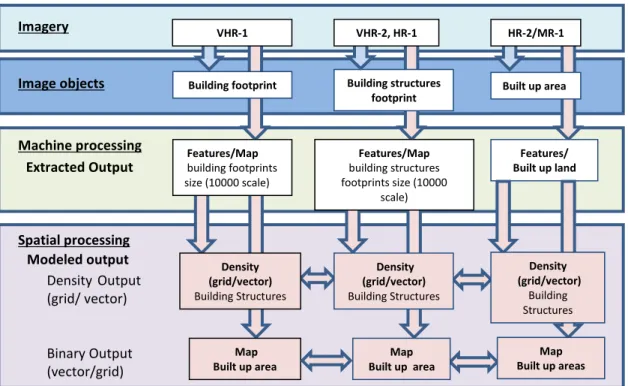
Figure 1. Conceptual satellite imagery processing workflow with input and output products labeled based on the terminology discussed in this report
Building footprint Building structures
footprint Built up area
Image objects Imagery Features/ Built up land Extracted Output Machine processing Map Built up area Density Output (grid/ vector) Binary Output (vector/grid) Density (grid/vector) Building Structures Density (grid/vector) Building Structures Density (grid/vector) Building Structures Modeled output Spatial processing Features/Map building structures footprints size (10000 scale) VHR-1 VHR-2, HR-1 HR-2/MR-1 Features/Map building footprints size (10000 scale) Map Built up area Map Built up areas
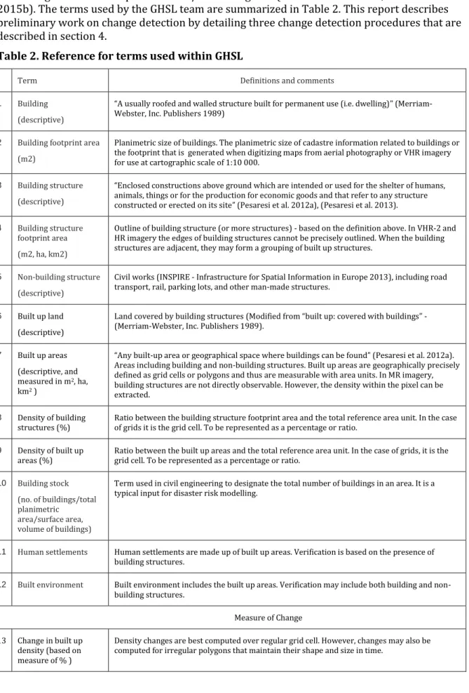
The processing chain developed by the JRC GHS team to process VHR-2, HR-1 images is extensively described in (Ferri et al. 2014, Florczyk et al. 2015, Pesaresi et al. 2013), while the processing chains used to process HR-2/MR-1 images in (Pesaresi et al. 2015a, Pesaresi et al. 2015b). The terms used by the GHSL team are summarized in Table 2. This report describes preliminary work on change detection by detailing three change detection procedures that are described in section 4.
Table 2. Reference for terms used within GHSL
Term Definitions and comments
1 Building (descriptive)
“A usually roofed and walled structure built for permanent use (i.e. dwelling)” (Merriam-Webster, Inc. Publishers 1989)
2 Building footprint area (m2)
Planimetric size of buildings. The planimetric size of cadastre information related to buildings or the footprint that is generated when digitizing maps from aerial photography or VHR imagery for use at cartographic scale of 1:10 000.
3 Building structure (descriptive)
“Enclosed constructions above ground which are intended or used for the shelter of humans, animals, things or for the production for economic goods and that refer to any structure constructed or erected on its site” (Pesaresi et al. 2012a), (Pesaresi et al. 2013).
4 Building structure footprint area (m2, ha, km2)
Outline of building structure (or more structures) - based on the definition above. In VHR-2 and HR imagery the edges of building structures cannot be precisely outlined. When the building structures are adjacent, they may form a grouping of built up structures.
5 Non-building structure (descriptive)
Civil works (INSPIRE - Infrastructure for Spatial Information in Europe 2013), including road transport, rail, parking lots, and other man-made structures.
6 Built up land (descriptive)
Land covered by building structures (Modified from “built up: covered with buildings” - (Merriam-Webster, Inc. Publishers 1989).
7 Built up areas
(descriptive, and measured in m2, ha,
km2 )
“Any built-up area or geographical space where buildings can be found” (Pesaresi et al. 2012a). Areas including building and non-building structures. Built up areas are geographically precisely defined as grid cells or polygons and thus are measurable with area units. In MR imagery, building structures are not directly observable. However, the density within the pixel can be extracted.
8 Density of building
structures (%) Ratio between the building structure footprint area and the total reference area unit. In the case of grids it is the grid cell. To be represented as a percentage or ratio.
9 Density of built up
areas (%) Ratio between the built up areas and the total reference area unit. In the case of grids, it is the grid cell. To be represented as a percentage or ratio.
10 Building stock
(no. of buildings/total planimetric
area/surface area, volume of buildings)
Term used in civil engineering to designate the total number of buildings in an area. It is a typical input for disaster risk modelling.
11 Human settlements Human settlements are made up of built up areas. Verification is based on the presence of
building structures.
12 Built environment Built environment includes the built up areas. Verification may include both building and
non-building structures.
Measure of Change 13 Change in built up
density (based on measure of % )
Density changes are best computed over regular grid cell. However, changes may also be computed for irregular polygons that maintain their shape and size in time.
3.
Change detection for human settlements spatial growth
study
The growth of human settlements may be spatial and/or vertical. Vertical growth refers to buildings extending in elevation, while spatial refers to adding new buildings. The measurement of vertical growth requires VHR imagery and specialized processing that is not treated in this document. This work addresses the measurement of the spatial location and size of buildings and the changes over time. This additional encroaching of building structures on undeveloped land is what is referred as settlement spatial growth in time. From a measurement point of view, this is referred to as change detection and it can be quantified through image processing. From a mathematical point of view, the change analysis may have three possible outcomes: No change, Densification and Thinning. From the application point of view, the outcomes are better described using an additional variant for each mathematical outcome considering the “0” density options.
Let D be the BU density value of a cell (pixel) and consequently, D0 the BU density value in the
initial image, acquired at date t0, and D1 the BU density value in the final image, acquired at date
t1. The possible transitions for change detection operations are: No change (N), Thinning (T)
and denSification (S), as shown in Table 3.
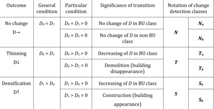
Table 3. Change detection classes for built up analysis
Outcome General condition
Particular condition
Significance of transition Notation of change detection classes No change D→ D0 = D1 D0 = D1 > 0 No change of D in BU class N Na D0 = D1 = 0 No change of D in non BU class Nb Thinning D↓ D0 > D1 D0 > D1 > 0 Decreasing of D in BU class T Ta D0 > D1 = 0 Demolition (building disappearance) Tb Densification D↑ D1 > D0 D1 > D0 > 0 Increasing of D in BU class S Sa D1 > D0 = 0 Construction (building appearance) Sb From the application point of view, the three possible outcomes are found in similar situations.
(1)No change - built up areas do not grow or decrease (Na). The no built up land remains
also unchanged (Nb).
(2)Thinning – built up areas decrease in size and is experienced in war and disaster affected zones (Ta) or rapidly growing cities that allocate section of cities to
undeveloped land (Tb).
(3)DenSification – increase in built up areas. The most common process of densification is urban sprawl. The increase of density from a non-zero value has a direct implication for the size of spatial extent of human settlements (Sa). The changes from no built up - to
built up is what is referred to as spatial urban growth or spatial growth as mentioned before (Sb).
Based on the above, the change from no buildings density is here reported as a change in built up area and thus in settlement extent.
The changes can then be computed differently depending on the datasets and on the processing chains available within GHSL. The change may be computed at different levels of the processing chains. Three preliminary procedures applied on two test sites are presented in this document and are conceptually illustrated in Figures 2 and 7. Each procedure differs because of the input data and/or the processing algorithm applied, being separately described in section 4. The first test case study uses imagery with two different resolutions, 10 m and 2.5m, and thus allows comparing imagery collected 30 years apart. In the second test case study, building structures density outputs of the GHSL methodology are processed through two different change detection procedures which are suited for processing imagery of comparable resolution, original 10m and aggregated 100m, 500m and 1km cell sizes.
Change detection methods
Change detection is the process of identifying differences in the state of an object or phenomenon by observing it at different times (Singh 1989). The remote sensing change detection methods can provide useful information on changes in area of land cover types, as well as on rate of change, spatial distribution of changed types, change trajectories of land-cover types, and an accuracy assessment of their results can be accomplished (Lu et al. 2014, Lu et al. 2004).
Urban monitoring implies multi-temporal observation and measurement of transformations or consistencies within built up areas. Remotely sensed data are well suited to provide information on urban land cover characteristics, and their changes over time, at various spatial, spectral and temporal scales. These data can assure timely and accurate change detection of built up
features, which is very important for understanding relationships and interactions between human and environment in order to promote better decision making. The taxonomy of the causes of radiometric changes in VHR images (Bruzzone & Bovolo 2013) identifies changes due to image acquisition conditions and those that occurred on the ground. This document focuses on detecting the changes occurring on the ground that are related to anthropic activity namely those related to built up structures and settlements.
The spatial resolution of VHR images are particularly suited for built up analysis as they allow to identify man made structures that are not detectable in images with moderate or high spatial resolution. The improved spatial resolution brings also an increased complexity and
heterogeneity in the satellite images. The definition of the change detection task becomes thus more complex and there is a strong need for the definition of new change detection methods being able to properly handle the high amount of spatial information. In VHR images, the geometrical details strongly emphasize the possibility to identify changes that are often not related to changes occurred on the ground or may be associated with changes not relevant to the specific application. Thus, it becomes mandatory to modify the perspective from the extraction of changes to the extraction of changes with a semantic meaning of interest for end-users. Regarding this aspect, the classes of change specific to our application field are defined in the Table 3, which presents their semantic meaning.
The input information used in our change detection process is the built up density derived from the Global Human Settlement Layer, GHSL (Pesaresi et al. 2012a, Pesaresi et al. 2013). This layer corresponds to the highest abstraction information - the object level (Bruzzone & Bovolo 2013) and is obtained by combining geometric primitive level features. By increasing the abstraction level, the dependency from the sensor and the acquisition condition decreases, whereas the one with respect to the ground condition is preserved. The built up density map, as a high level semantic layer, can be seen as a simplification of the original images reducing the high
variability that characterizes the radiometry at pixel level and therefore the dependency on the sensor properties and the acquisition conditions. However the problem of registration noise remains to be considered, as this influences the threshold selection.
In this work, based on a preliminary analysis of the most used change detection methods (Principal Component Analysis, PCA, Image Differencing Comparison, IDC, and Post-Classification Comparison, PCC), we discuss the results and try to identify future research directions for developing an appropriate approach for our GHS data type.
PCA change detection method belongs to the Transformation category (Lu et al. 2004) and reduces data redundancy between bands and emphasizes different information in the derived components. It assumes that multi-temporal data are highly correlated and change information can be highlighted in the new components. It cannot provide a complete matrix of change class information. Another disadvantage is the difficulty in interpreting and labeling the change information on the transformed images. The IDC and PCA methods, detecting binary
change/non-change information, extract only three classes S, T and N, (see Table 3), and they have common problems in thresholds selection.
IDC change detection method belongs to algebra category (Lu et al. 2004) and is relatively simple, straightforward, easy to implement and interpret, but it cannot provide complete
matrices of change information for accuracy assessment. The method consists in subtracting the first date image from a second-date image, pixel by pixel. In our case the pixel value is given by GHSL that takes profit from local textural and morphological features. The main disadvantage is the difficulty in selecting suitable thresholds to identify the changed areas.
PCC change detection method, detecting detailed “from-to” change information, extracts in our case four classes; S, T, Na and Nb. With appropriate post-processing, it is possible to obtain all
the six classes from Table 3. The method consists in separately classifying multi-temporal images into thematic maps, then in implementing comparison of the classified images, pixel by pixel. The method has the advantages of minimizing impacts of atmospheric, sensor and
environmental differences between multi-temporal images and of providing complete matrix of change information. As disadvantages, the method requires time and expertise to create useful classification products. The final accuracy depends on the quality of the classified image of each date. Once again the key factor is the correct threshold selection to create an accurate thematic classification images, prior to PCC change detection method.
4.
Change Detection tests
This section presents and discusses preliminary results of the three change detection methods mentioned above, and tries to identify future research directions for developing an appropriate approach for GHS type of result images. The two used datasets contain SPOT images which were differently processed and they depict Alger and Dublin city areas.
4.1.
Alger case study
The Alger case study aims to show the potential of automatic built-up mapping and change detection using SPOT imagery. The test is carried out on one city and its surroundings as a proof of concept. However, the availability of SPOT archives data allows extending the test for those regions of the world for which SPOT-1 data was collected starting from 1986. This test also aims to show the potential for change detection from datasets with different spatial resolutions within the range of VHR to HR. While the test is carried out on one city only, the concepts and procedures for change detection can be applied to detect changes in continental datasets. SPOT imagery is a popular datum to detect changes of the built environment. It has been used for producing land use land cover maps and then changes of the spatial extent of each cover class within the map over time. Some authors have also attempted to measure the changes only for the built environment (Tiede et al. 2012). Finally, a new research area is opening where changes are measured by directly comparing the images or features derived from the imagery (Gueguen et al. 2013), (Ehrlich & Bielski 2011). This research follows this latest trend.
The two SPOT images used to address changes in Alger were collected by SPOT-1 on 8th July
1986 and by SPOT-5 on 9th February 2009. The 1986 image was available as a panchromatic
band at 10 m resolution and the second as a panchromatic band at 2.5 m resolution. SPOT also provides multispectral bands in coarser spatial resolution with respect to the panchromatic image that were not available for this analysis. The multispectral bands typically refine the built up detection and should be used in future change detection procedures. The common area of the two images accounts for of 12.000 km2 over which the change detection was analyzed
(Figure 3).
4.1.1.
Methodology
This test uses a change detection method for imagery from different sensors that was originally applied over Casablanca (Ehrlich & Bielski 2011). It was selected herein for its robustness that allows comparing imagery at different resolutions. Other techniques were also considered but they required data of similar spatial resolution that were not available here (Gueguen et al. 2011). The relative simplicity of the techniques also helps in better understanding the potential of information content in the imagery.
The processing procedure is based on a number of steps as illustrated in Figure 2. (1) Pre-processing imagery for geometric correction (in order to make the measures comparable, we degraded the 2.5 m resolution to 10 m). (2) Calculation of built up presence index (BUPI) features (Pesaresi et al. 2008). (3) Combining (stacking) the BUPI features into a single two band image in order to compute principal component analysis (PCA). (4) Processing the second principal component (PC2) as a change-feature; (5) Modeling the change feature based on a grid scale. The main processing relates to the computation of a texture-related feature - Pantex (Pesaresi et al. 2008). It provides continuous values of texture measurements from the original input band. The derived texture information was shown to be highly correlated with built up land. The size of the built up structures and their spatial arrangements at the spatial resolution of SPOT maximize that texture information. The BUPI features thus record high level of texture opposed to other land covers where textures are low. The texture features have shown to be robust also when computed over images collected from different sensors as in this case.
Figure 2. Conceptual flowchart following that of Figure 1 used to compute change in Alger
Pantex
PC_2 change feature BU Feature
Binary - Change Binary BU
Grid change Grid BU
The change analysis assumes that the textures computed at different times can be compared to identify changes in textures and thus changes in built up. This work is based on the assumption that the first principal component (PC1) captures the regions on the image with similar textures while the second component, the changes in textures and thus changes in built up between the two acquisition dates. We analyzed only the positive changes (S class) that assume a change from low texture as in agricultural land into landscapes with high texture as in built up land. Thresholds were applied on the PC2 corresponding to the Change features and on the Pantex of the 2009 in order to obtain respectively a binary change and a binary built up map for 2009. The changes were then further processed and aggregated at grid intervals of a grid of 100 m cell size. This allows to fine tune the changes by removing unwanted artifacts corresponding to small patches or those whose change signal is of low magnitude. The artifacts are inevitable given the technical characteristics of the imagery. The aggregation to a standardized spatial unit of 100 m will facilitate the comparison with outputs that will be obtained from other future measurements.
4.1.2.
Results
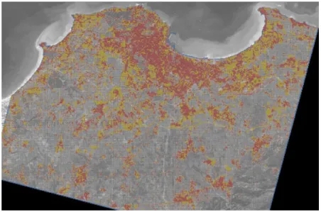
The results are visually depicted in Figures 3 and 4. Figure 3 shows the intersection of land of the two SPOT images for a total of 1200 km2, as well as the built up layer and the changes for the
entire metropolitan region. The image is suited for cartographic reproduction at 1: 250 000 scale.
Figure 3. Alger and settlements surrounding Alger over a 52 x 40 km2 area. The settlement maps are labeled red for built up before 1986 and yellow for built up after 1986.
Figure 4 shows a selected study area of 9 km2 with the images from 1986 (a) and 2009 (b), the
built up in 2009 (c), the built up increase overlaid on the 1986 image (d) and on the 2009 image (e), as well as the built up map and change map combined (f).
Figure 4. SPOT-1 (a) and SPOT-5 (b) imagery over an area of 3 x 3 km2 in the periphery of Alger. The image shows in red (c) the settlement map computed in 2009 and in yellow the change in built up from 1986 overlaid first on the 1986 SPOT image (d) and then on the 2009 SPOT image (e), while(f) shows the built up and change combined.
The maps provided allow generating statistics on urbanization. The maps have not been validated quantitatively due to a lack of reference data both for 1986 and for 2009. However, the maps have been visually inspected against the imagery from which the change was
produced as shown in Figure 4. The statistics that are generated are only tentative and need to be confirmed through a thorough validation protocol. The analysis shows that 339.69 km2 (i.e.
100 x 100 m2 grid cells) are measured as BU in 1986. In only 23 years, 173.80 km2 are added to
the BU land of 1986. That is an increase of 50% when compared to the BU of 1986. The total built up land over the area increases from just over 26% to nearly 40% in 2009. The statistics are based on the analysis of built up land computed over 100 grid cells. Considering that the information has been binary as no-built up (“0” value) and built up (above “0” value), these preliminary statistics need to be treated with caution. In fact, different density thresholds or different grid cell sizes used in the analysis may provide results that may differ from those provided herein.
Table 4. Built up and built up change statistics over the Alger metropolitan area. Date In 1986 1986-2009 In 2009 No. of hectares 33969 17380 51349 Percentage over total 26.39 13.50 39.89
4.1.3.
Discussion
The Alger case study tests a conceptual model for quantifying built up areas and changes in time from multi-resolution remote sensing. It is tested on VHR2 and HR imagery. The spatial
resolution of the imagery assumes that the large majority of the buildings can be detected using automatic techniques. The processing aims to provide features that are related to the building density. The features can then be modeled to provide density of built up and changes. The selection of the input datum, the processing techniques, the modeling procedure that includes
a b c
the grid cell size which defines the density and the spatial rules used will determine the final outcome.
The visual analysis of SPOT-5 panchromatic imagery used as t1 image confirms that the building structures can be enumerated. The spatial arrangement of buildings can also be clearly
assessed and thus the built up land can be measured. The visual analysis of SPOT-1
panchromatic imagery used as t0 image, on the other hand, shows that the visual detection of built up structures from the SPOT-1 data is much more challenging. While large buildings may be identified and mapped, the single building structures are more difficult to recognize. The automatic procedure to detect the building structures from SPOT-5 may perform better but the challenges remain. The change detection technique – that combines features calculated from SPOT-1 and SPOT-5 - provides a relative unambiguous result when the changes in built up between t0 and t1 occur through building encroachment (natural land is converted in dense built up land). The small density changes are difficult to assess due to the characteristics of the data and to the absence of reference data.
In general, given the different spatial resolution and the seasonal variations between the two acquisitions, it is remarkable that the changes can be detected. Further refinement of the techniques and interpretation is needed. The ultimate goal of this work is to walk through the conceptual change model, test the process rather than the technique and/or the result. The final map and the final statistics are not definitive also because no reference data are available for benchmarking. Each step of the procedure will be further evaluated to better understand the information content of the imagery, the techniques used to measure changes and the eventual outcome to be used in urbanization studies.
4.2.
Dublin case study
The Dublin case study uses image differencing comparison, IDC, and post-classification comparison, PCC, methods to accomplish change detection in the case of a time series
containing three remote sensing images acquired on Dublin area. The first method makes a pre-classification direct comparison between pairs of GHSL transformed images, while the second method extracts the changes through comparison of two classification images in BU and non BU classes. Both methods have as input data the GHSL transformation results of satellite images but their advantages and drawbacks are quite opposite. The pre-classification method avoids the errors introduced by the second method where inaccuracies in classification are propagated into the change analysis. The post-classification comparison methods can bypass the difficulties in change detection associated with the analysis of images affected by seasonality or by
difference in sensor. This is why it is useful to compare the results of these methods. Because the accuracy of both methods is influenced by the selected level of the used thresholds, a special attention is paid to this problem. Also, having three dates of acquisition and consequently three image pairs to be compared, the compatibility (consistency) of change detection results implies the correlation of the used thresholds and a procedure to assess this was developed.
Change detection is a procedure that requires careful design of each step, including the statement of research problems and objectives, data collection, preprocessing, selection of suitable change detection algorithms, and evaluation of the results. Errors or uncertainties may emerge from any of the steps, thus affecting the change detection results.
The accuracy assessment for change detection is particularly difficult due to problems in collecting reliable temporal field-based datasets (in our case cadastral data). In absence of this data type, the change detection cannot provide quantitative analysis of the research results.
4.2.1.
Input data and preprocessing
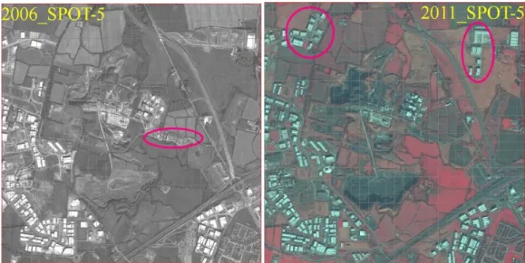
The three VHR-2 SPOT-5 images used to address changes in Dublin area belong to the pan-European Copernicus (formerly Global Monitoring for Environment and Security - GMES) datasets produced in support to the Urban Atlas project (Urban Atlas project 2006, 2012). The
oldest two images were available as panchromatic bands at 2.5m spatial resolution and were acquired on 16th September 2006 and on 12th September 2009. They belong to a dataset used
for the production of Urban Atlas 2006 which contains 711 SPOT-5 images from the period 2004 – 2010 (84 panchromatic images, 627 multispectral images). The third image was available as a multi-spectral scene pre-processed in pan-sharpened mode at 2.5m spatial resolution, acquired on 24th February 2011, being part of the GMES Core_003 VHR2 dataset
(Burger et al. 2012) used for the production of Urban Atlas 2012. For this study, we have selected an area of 30x30 km2 centered on Dublin metropolitan area, presented in Figure 5 (left
side). The derived products used as input for the change detection procedures were obtained following the GHSL general methodology (Pesaresi et al. 2012a, Pesaresi et al. 2013) with some specific modifications made to optimize the exploitation of the available imagery (Ferri et al. 2014, Florczyk et al. 2015). They are represented by a continuous information layer at 10m spatial resolution resulted from aggregating, using an average operator, the 2.5m boolean outputs of the GHSL workflow. Each pixel value expresses the proportion of the pixel area covered by buildings (density of building structures).
For a good implementation of change detection analysis, some important conditions must be satisfied regarding data preprocessing: precise registration of multi-temporal images, precise radiometric calibration or normalization and atmospheric correction between the multi-temporal images, selection of the same spatial and spectral resolution images with very near anniversary acquisition dates if possible. In our available data, besides the possible errors in registration and calibration, there is a seasonality problem.
In order to see the influence of map scale on change detection results, the cell size was increased, in steps, from 10m to 1km. Thus is possible to observe the under/over estimation effects on results.
Fig. 5 The original 2011 SPOT-5 image with 2.5m spatial resolution (left side) and the corresponding 10m GHSL map (3 x 3km2 zoom location in red)
To better analyze the BU changes, the study was focused on a 3 x 3 km2 zoomed area marked in
Figure 5. The reason for the choice of the zoom location was the presence of an isolated building – the airport – upper right side of 2011 image of the Figure 6, and of a well-defined building assembly – upper left side of the same 2011 image – appeared in the studied time period, and of a demolition zone marked in 2006 image (Figure 6, left side). The presence of corresponding classes of these modifications in these locations was observed during the increase of cell size from 10m to 1km
.
Fig. 6 The most visible built up changes in the zoomed area in the 2006-2011 time period.
4.2.2.
Methodology
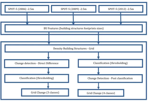
The main processes used for change maps determination for Dublin area are presented in Figure 7. Starting from the SPOT-5 images with 2,5m resolution for 2006, 2009 and 2011 years, are obtained the GHSL images containing the density of building structures and having a 10m resolution which represent the input of the change detection procedures.
Fig. 7. Conceptual flowchart used to compute change in Dublin area.
Considering the built up density map at 10m cell size, the starting map of our study, the area covered with built up structure rises with 7.27% in the 2006_2011 time period with a major contribution of 2009_2011 time period. In the case of PCC approach, the applied threshold of 10% from “pixel” value leads to a decrease of built up structure in the range 4.5% - 5% for all acquisition years. In this situation, for the transition 2006_2011 there is an increase of built up area with 6.91%.
The flowchart diagram shows two processing chains for change detection procedures. In the direct difference change approach, the result images are classified in three classes, Thinning, T,
No change, N, and denSification, S, according to the notation from Table 3. This classification is made by value domain thresholding via B1 (for minimum value) and B2 (for maximum value) thresholds (Breaks).
In the case of Change Detection on GHSL images, the obtained histograms are very sharp in shape, with an over populated central bin (situated around “0” value). The histogram shape normally depends on the resolution level given herein by different aggregation levels. Rising artificially (simulating) the cell size from 10m to 1km, the cell values domain decreases from (-1, 1) for 10m cell size to (-0.02, 0.03) for 1km cell size. Due to the aggregation by averaging of pixel values, made for obtaining a value for a bigger cell, the population percentage of the central bin decreases from more than 70% for 10m resolution to around 20% for 1km resolution. This kind of “smoothing” is responsible for information dilution leading to loss of information.
The IDC change approach requires selection of thresholds to differentiate change from non-change areas. The thresholds can be defined with a manual or statistical procedure. In the manual trial-and-error procedure - referred also as interactive procedure - an analyst interactively adjusts the thresholds and evaluates the resulting image until satisfied. The
Change detection - Direct Difference
Change Detection - Post classification
Grid Change (3 classes) Grid Change (4 classes) Classification (thresholding)
Classification (thresholding) Density Building Structures - Grid
BU Features (building structures footprints sizes)
statistical procedure can automatically select the threshold based on statistical measures or other characteristics of the change detection histogram.
We studied several threshold selection procedures according to histogram characteristics in order to construct an automatic method. The results of two methods used to establish the B1
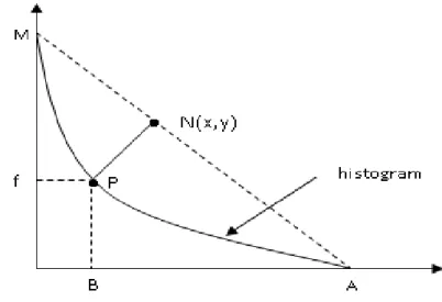
and B2 threshold values are presented here: the Natural Breaks, NB and the triangle method with variants. The first method, NB, uses the Jenks' Natural Breaks algorithm (Jenks 1967) intended for extracting classes according to the natural groupings inherent in the data. Class breaks are identified that best group similar values and that maximize the differences between classes (they minimize each class’s average deviation from the class mean, while maximizing each class’s deviation from the means of the other groups). Due to the fact that T and S class population obtained with NB technique are quite large, but their difference doesn’t reach the level of BU structure appearance from the global analysis presented earlier, we tried the triangle method, a shape-based method proposed by Rosin (Rosin 2001) and inspired from the triangle algorithm (Zack et al. 1977). A straight line, MA, is drawn from the maximum to the end of the histogram, to form a triangular-like shape (see Figure 8).
Fig. 8 The triangle method
The threshold is selected at the point of the histogram that maximizes the perpendicular distance NP from the histogram to the straight line MA. This method is used for both wings of histogram to obtain the value of thresholds B1 and B2. The method gives suitable results, but tends to be sensitive to parameters such as the statistical fluctuations of the histogram, and the position of the endpoint (highest or lowest gray level). In our case, the discontinuous statistical distribution represented by a jagged histogram increases the probability of error when
determining the threshold value B.
Using the histogram peak, M, as highest point for the straight line, the thresholds value B1 and
B2 are close to those obtained with NB method and with the same problem of overestimation. That is why we tried to “smooth” the histogram decreasing the peak frequency value, M. The obtained result for M/2 frequency is very similar to the previous one. The other values for highest point were those of adjacent bins to the histogram peak, denoted with sM. The
corresponding frequencies for sM points are usually more than ten times lower than for M and the results are reported herein.
At continental or global scale, coarse resolution data are usually used for change detection. Using in input HR or VHR data, larger scales may overcome some misregistration and miscalibration errors. In order to evaluate the influence of map scale on change detection results, the cell size was increased from 10m to 1km. The 1km aggregated density used a value aggregation function. The changes were then computed for maps at grid sizes of 100m, 500m
and 1km. So, it is possible to observe the under/over estimation effects of scale variation on the change detection results.
In the post-classification comparison change detection approach the input data are the built up and no-built up classes obtained with 10% threshold value of the density of building structures of the GHSL images. The transition from 2.5m to 10m cell size means averaging the values of 16 small cells for a larger one. Applying a threshold of 10% means in fact that there are not taken into account for built up labeling the 10m cells that contain only one, isolated built up 2.5m cell. The changes are extracted through comparison of the classification results. The results of this approach are directly expressed in four classes: Na, Nb, T and S with the notations of Table 3. So,
this method directly discriminates between classes Na and Nbfrom the class N of the previous
approach while it merges the subclasses Ta and Sa(intra-class change is not defined) inside the
BU no change class Na. The change detection maps for larger cell sizes are obtained with
majority vote procedure.
The main problems raised in the processing chains are the special shape of change detection histogram and consequently difficulties in selecting appropriate threshold values for image differencing comparison approach, and the aggregation technique for post-processing approach.
4.2.3. Results
Applying the two change detection approaches, the image differencing comparison and post-classification comparison procedures, we obtained the results summarized in Tables 5 and 6. The change extraction results allow detecting changes, identifying the nature of the change, measuring the areal extent of the change, and assessing the spatial pattern of the change. This allows evaluating dynamics, direction, rate and spatial pattern of built up changes.
Considering the built up density map at 10m cell size, the starting map of our study, the area covered with built up structure rises with 7.27% in the 2006_2011 time period with a major contribution of 2009_2011 time period. In the case of PCC approach, a preliminary global assessment of building structures areas from the input images with the applied threshold of 10% from “pixel” value leads to a decrease of built up structure in the range 4.5% - 5% for all acquisition years. In this situation, for the transition 2006_2011 there is an increase of built up area with 6.91%.
In the case of IDC approach, the increase of cell dimension for Natural Breaks (Jenks) threshold generally leads to the increase of BU Appearance, S, and BU disappearance, T, classes in a given change detection period, and consequently, the decrease of no change class, N.
In the case of the PCC approach, the increase of cell size leads to the disappearance of weakly populated classes (T - 0.00%) for larger cell size – a loss of information – and to the increase of NBU no change class, Nb, for 10, 100, 500m cell sizes. It can also be noticed that the biggest value
of NBU no change class, Nb, is in 2006_2009 time period for all cell sizes and the smallest value
of BU Appearance class, S, is in 2006_2009 time period for all cell sizes, fact that leads to the conclusion that the construction rate increased after 2009.
Table 5. The percentage of three extracted classes’ area with IDC change detection for different cell sizes and threshold types.
Cell
size Threshold type Period NB 2006_2009 sM NB 2009_2011 sM NB 2006_2011 sM
10m BU Thinning (T) 7.42 1.48 7.64 1.68 7.50 1.65
BU Densification (S) 7.66 2.19 8.69 2.63 9.13 2.53 100m BU Thinning (T) 8.68 2.58 11.27 2.69 10.96 1.33 No change (N) 81.35 93.85 81.20 93.85 79.97 97.28 BU Densification (S) 9.97 3.57 7.53 3.46 9.07 1.39 500m BU Thinning (T) 11.25 2.36 15.92 6.19 14.42 5.61 No change (N) 73.42 91.72 76.00 88.14 71.69 91.06 BU Densification (S) 15.333 5.92 8.08 5.67 13.89 3.33 1km BU Thinning (T) 14.33 5.33 19.11 8.00 19.44 8.22 No change (N) 65.45 81.33 67.89 84.11 65.67 68.33 BU Densification (S) 20.22 13.34 13.00 7.89 14.89 23.45
Table 6. The percentage of four extracted classes’ area with PCC change detection for different cell sizes.
Cell size Class 2006_2009 2009_2011 2006_2011 10m BU_Thinning (Tb) 6.05 2.79 3.68 NBU_No Change (Nb) 73.73 72.21 71.33 BU_No Change (Na) 14.37 17.44 16.75 BU_Densification(Sb) 5.85 7.56 8.24 100m BU_Thinning (Tb) 1.62 0.38 0.52 NBU_No Change (Nb) 75.97 73.83 73.69 BU_No Change (Na) 20.81 22.03 21.90 BU_Densification(Sb) 1.60 3.76 3.89 500m BU_Thinning (Tb) 0.89 0.03 0.00 NBU_No Change (Nb) 77.58 73.94 73.97 BU_No Change (Na) 20.42 21.5 21.31 BU_Densification(Sb) 1.11 4.53 4.72 1km BU_Thinning (Tb) 0.22 0.00 0.00 NBU_No Change (Nb) 79.78 73.33 73.33 BU_No Change (Na) 19.44 20.00 19.67 BU_Densification(Sb) 0.56 6.67 7.00
The results for both change detection methods summarized in Tables 5 and 6 allow a
comparison between the approaches. The direct differencing approach reveals three classes, T,
N, and S while the post-classification comparison approach highlights 4 classes. The PCC approach makes a supplementary discrimination inside the N class by revealing the Na and Nb
subclasses (see also, Figure 9) but the subclasses Ta and Saare now merged inside the BU no
change class Na. For the direct differencing case, the discrimination inside the T and S classes
will imply additional post-processing. The results of both approaches essentially depend on thresholds selection. Generally, in image differencing comparison approach the Natural Breaks, NB, technique leads to a large overestimation of T and S classes, and the sub-Maxim, sM, technique leads to underestimation of T and S classes. The 10% thresholds used in post-processing approach for NBU/BU classification generally lead to intermediate estimation of