Open Access Dissertations Theses and Dissertations
January 2015
Scaling Up Network Analysis and Mining: Statistical Sampling,
Scaling Up Network Analysis and Mining: Statistical Sampling,
Estimation, and Pattern Discovery
Estimation, and Pattern Discovery
Nesreen Kamel AhmedPurdue University
Follow this and additional works at: https://docs.lib.purdue.edu/open_access_dissertations
Recommended Citation Recommended Citation
Ahmed, Nesreen Kamel, "Scaling Up Network Analysis and Mining: Statistical Sampling, Estimation, and Pattern Discovery" (2015). Open Access Dissertations. 1445.
https://docs.lib.purdue.edu/open_access_dissertations/1445
This document has been made available through Purdue e-Pubs, a service of the Purdue University Libraries. Please contact [email protected] for additional information.
PURDUE UNIVERSITY GRADUATE SCHOOL Thesis/Dissertation Acceptance This is to certify that the thesis/dissertation prepared
By Entitled
For the degree of
Is approved by the final examining committee:
To the best of my knowledge and as understood by the student in the Thesis/Dissertation Agreement, Publication Delay, and Certification Disclaimer (Graduate School Form 32), this thesis/dissertation adheres to the provisions of Purdue University’s “Policy of Integrity in Research” and the use of copyright material.
Approved by Major Professor(s):
Approved by:
Head of the Departmental Graduate Program Date Nesreen Kamel Ahmed
Scaling Up Network Analysis and Mining: Statistical Sampling, Estimation, and Pattern Discovery
Doctor of Philosophy Jennifer Neville Chair Christopher W. Clifton Walid G. Aref Sonia Fahmy Jennifer Neville
STATISTICAL SAMPLING, ESTIMATION, AND PATTERN DISCOVERY
A Dissertation Submitted to the Faculty
of
Purdue University by
Nesreen K. Ahmed
In Partial Fulfillment of the Requirements for the Degree
of
Doctor of Philosophy
August 2015 Purdue University West Lafayette, Indiana
To my mother and the loving memory of my father They are the ones who made me who I am today
ACKNOWLEDGMENTS
I am extremely thankful and honored to be surrounded by so many exceptional and inspirational people. I believe words are not enough for expressing my gratitude to them. First and foremost, I am extremely fortunate to have my PhD advisor Jennifer Neville, for her continuous support, insightful feedback, invaluable advice over the years of my PhD journey, and for challenging me and encouraging me to find my way as a researcher. I can never thank my PhD committee members enough for their support and guidance. I am very grateful to Sonia Fahmy, Chris Clifton, and Walid Aref, for their invaluable feedback and advice that improved my dissertation and their encouragement over the years. I am thankful for them for always finding new ways to consider a problem.
I have had enjoyable, rewarding discussions, and collaborations with many professors during my PhD. I was very fortunate to work with Ramana Kompella, and I am extremely grateful for his guidance that ultimately helped me become a better researcher. I am particularly indebted and honored to have the opportunity to work with Nick Duffield. Nick has been a great mentor to me and I learned a lot from him. I can never thank Nick enough for his continuous guidance, support, and encouragement.
I specially like to thank Ahmed Elmagarmid, Greg Frederickson, Alan Qi, SVN Vish-wanathan, Luo Si, David Gleich, and Susanne Hambrusch for all their support and guidance. I am very grateful for Mohammad Al Hasan for his kind nature, advice, and collaboration. Special thanks to Dr. Groman for his support, advice, and guidance during my PhD.
Special thanks to Sebastian Moreno, Dan Zhang, Mohamed Yakout, Tao Wang, Hyokun Yun, Rongjing Xiang, Hoda Eldardiry, Timothy La Fond, Joel Pfeiffer, Hogun Park, Iman Alodah, Praveen Kumar, Camille Gaspard, Sait Celebi, Suvidha Kancharla, Ellen Lai, Giselle Zeno, Pablo Granda, Jiasen Yang, Jason Meng, Ahmed Aly, and many others, for the interesting discussions and the great times during conferences and/or meetings.
I feel very grateful to have had the opportunity to work closely with top researchers in a variety of industrial labs. I am especially fortunate and honored to have the opportunity
to work with Ayman Farahat at Adobe Advanced Technology Labs. He has been a great mentor to me and I am especially thankful for his often selfless support, encouragement, and advice over the years.
In addition, I am especially fortunate to Robert Kuhn, my mentor at Intel, for his kind nature, advice, and encouragement. Robert helped me to pursue new applications for data mining beyond the traditional ones. I would also like to thank Al Mamunur Rashid for his friendship, encouragement, and collaboration during my time at Intel.
During my time at Facebook, I am extremely fortunate to have had the opportunity to be mentored by Rajiv Krishnamurthy. I am especially thankful for his help and encouragement that gave me the strength to overcome many challenging problems that I encountered at Facebook and beyond.
I feel eternally indebted to my early research advisor, Amir Atiya, who not only intro-duced me to research in data mining and machine learning, but has significantly changed my life in the process. Amir has been a great source of inspiration and true role model as a researcher, mentor, and friend. I thank him for his relentless and selfless advice to tackle difficult problems. His caring nature always gave me the strength to move forward even during the tough times.
During my time at Purdue, I have built friendships that I hold closely to my heart. I thank Nilothpal Talukder, Balamurugan Anandan, Hani Jibrin, Sohayla Jibrin, Lamis Be, Ali Roumani, Muna Albasman, Sereen Al-Khalili, Ahmed Abdelhamid and many others. I am indebted to Ryan Rossi for his friendship, encouragement, and collaboration.
Most of all, I owe my deepest gratitude to my family for their endless love and encour-agement. Everything was possible due to their strong support. I dedicate this work to my parents. My father has been always a continuous source of moral, joy, and support in my life. I believe he is still with me and I hope I make him proud. My mother has been so self-less in supporting me at all phases of my life and career. I am indebted to my sister Amany and brothers Mohamed and Mustafa for their continuous support and encouragement over the years. I have the best family anyone could ask for, and words will never be sufficient for expressing my gratitude to my family.
TABLE OF CONTENTS Page LIST OF TABLES . . . ix LIST OF FIGURES . . . xi ABSTRACT . . . xiii 1 INTRODUCTION . . . 1
1.1 Challenges of Network Analysis and Mining . . . 1
1.2 A Taxonomy of Network Sampling Methods . . . 3
1.2.1 Classes of Network Sampling Methods . . . 3
1.2.2 Spectrum of Computational Models . . . 4
1.3 Problem Statement . . . 8
1.3.1 Sampling from Large Static Graphs . . . 10
1.3.2 Sampling from Streaming Graphs . . . 11
1.3.3 Big Graph Analytics and Unbiased Estimation . . . 12
1.4 Contributions and Outline . . . 13
2 BACKGROUND . . . 15
2.1 Foundations and Notations. . . 16
2.2 Goals, Units, and Population of Networks . . . 17
2.3 Classes of Sampling Methods . . . 20
2.4 Evaluation of Sampling Methods . . . 22
2.5 Models of Computation. . . 27
2.6 Review of Related work . . . 31
2.6.1 Network Sampling in Social Science . . . 31
2.6.2 Statistical Properties of Network Sampling . . . 32
2.6.3 Network Sampling in Networked Systems . . . 32
Page
2.6.5 Graph Streams . . . 34
3 SAMPLING FROM LARGE STATIC GRAPHS . . . 36
3.1 Motivation . . . 36
3.2 Two-Pass Stream Sampling . . . 37
3.3 Analysis of Sampling Bias . . . 39
3.3.1 Selection Bias Toward High Degree Nodes . . . 39
3.3.2 Downward Bias Due to Sampling . . . 41
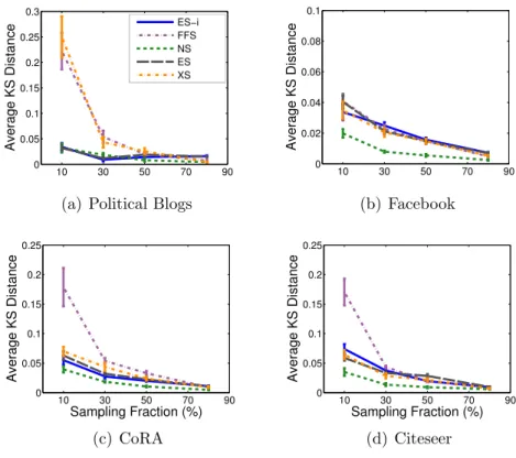
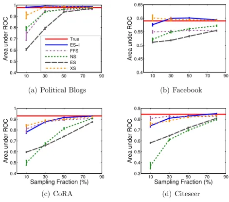
3.4 Experiments . . . 44
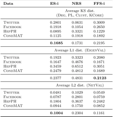
3.4.1 Distance Metrics . . . 45
3.4.2 Statistical Distributions . . . 46
3.4.3 Comparison to Metropolis Graph Sampling. . . 48
3.5 Network Sampling Designs for Relational Classification . . . 53
3.5.1 Impact on Parameter Estimation . . . 54
3.5.2 Impact on Classification Accuracy . . . 57
3.6 Summary . . . 59
4 SAMPLING FROM STREAMING GRAPHS . . . 61
4.1 Motivation . . . 61
4.2 Streaming Node Sampling . . . 62
4.3 Streaming Edge Sampling . . . 63
4.4 Streaming Topology-Based Sampling . . . 64
4.5 Partially-Induced Edge Sampling (PIES) . . . 65
4.6 Experiments . . . 68
4.6.1 Distance Metrics . . . 68
4.6.2 Statistical Distributions . . . 69
4.6.3 Analysis of Dense Versus Sparse Graphs . . . 75
4.6.4 Analysis of Isolated Nodes . . . 75
4.7 Sampling from Multigraph Streams . . . 78
Page
4.7.2 Statistical Distributions of Temporal Properties . . . 80
4.7.3 Interplay between Graph Dynamics and Structure . . . 82
4.7.4 Randomization Tests for Graph Streams . . . 84
4.8 Summary . . . 85
5 SAMPLE & HOLD: A FRAMEWORK FOR BIG GRAPH ANALYTICS 86 5.1 Motivation . . . 86
5.2 Relation to Classic Sample and Hold . . . 89
5.3 Framework for Graph Sampling . . . 90
5.3.1 Graph Stream Model . . . 90
5.3.2 Edge Sampling Model . . . 90
5.3.3 Subgraph Estimation . . . 91
5.4 Unbiased Estimation . . . 93
5.4.1 General Estimation and Variance . . . 94
5.4.2 Edges . . . 95
5.4.3 Triangles. . . 95
5.4.4 Connected Paths of Length 2 . . . 96
5.4.5 Clustering Coefficient . . . 96
5.4.6 Nodes . . . 97
5.5 Graph Sample and Hold . . . 97
5.5.1 Algorithms . . . 97
5.5.2 Illustration with gSH(p,1) . . . 99
5.6 Experiments . . . 100
5.6.1 Performance Analysis . . . 101
5.6.2 Confidence Bounds . . . 102
5.6.3 Comparison to Previous Work . . . 106
5.6.4 Effect ofp, q on Sampling Rate . . . 108
5.6.5 Implementation Issues . . . 109
Page
5.8 Summary . . . 113
6 FAST PARALLEL MOTIF COUNTING FOR LARGE GRAPHS . . . . 115
6.1 Motivation . . . 115
6.2 Motifs, Scalability, Applications . . . 116
6.3 Background . . . 118
6.3.1 Notations and Definitions . . . 118
6.3.2 Relation to Graph Complement . . . 121
6.3.3 Relation to Graph & Matrix Reconstruction Theorems . . . 121
6.4 Framework. . . 122
6.4.1 Searching Edge Neighborhoods . . . 122
6.4.2 Counting Motifs of Size (k = 3) Nodes . . . 123
6.5 Counting Motifs of Size (k = 4) Nodes . . . 126
6.5.1 Motif State Transition Diagram . . . 127
6.5.2 General Principle for Counting Motifs of sizek = 4 . . . 128
6.5.3 Analysis & Combinatorial Arguments . . . 131
6.5.4 Algorithm . . . 144
6.6 Experiments & Applications . . . 145
6.6.1 Scalability & Runtime . . . 146
6.6.2 Large-Scale Graph Comparison & Classification . . . 149
6.6.3 Finding Large Stars, Cliques, and Other Patterns . . . 150
6.7 Summary . . . 152
7 SUMMARY AND CONCLUSION . . . 163
7.1 Contributions . . . 164
7.2 Future Directions . . . 166
REFERENCES . . . 168
LIST OF TABLES
Table Page
2.1 Description of Network Statistics . . . 23
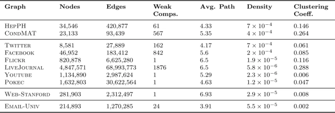
3.1 Characteristics of Network Data Sets . . . 44
3.2 Comparison of the Maximum Kcore Number for Static Graphs . . . 47
3.3 Comparison to Neighbor Reservoir Sampling . . . 52
4.1 Comparison of the Maximum Kcore Number for Streaming Graphs . . 71
4.2 Comparison of Percentage of Isolated Nodes for All Sampling Algorithms 76 4.3 Average KS Distance for Stream Sampling Methods. . . 77
4.4 Average L1/L2 Distance for Stream Sampling Methods.. . . 77
4.5 Characteristics of Multigraph Data Sets . . . 78
5.1 Estimation on a Path of Length 3 . . . 99
5.2 Statistics of Data Sets . . . 100
5.3 Estimated Properties using Graph Sample & Hold . . . 103
5.4 Coverage Probability for 95% Confidence Interval . . . 106
5.5 Comparison to Streaming Triangles . . . 107
5.6 Runtime for Sampling and Estimation using gSH . . . 110
6.1 Summary of Motif Notation and Properties . . . 120
6.2 Runtime & Statistics for a Subset of 55 Networks . . . 147
6.3 Accuracy of Graph Classification . . . 150
6.4 Statistics of Facebook100 Networks . . . 154
6.5 Statistics of Facebook100 Networks (Table 6.4 continued) . . . 155
6.6 Statistics of Biological, Co-authorship & Interaction Networks . . . 156
6.7 Statistics of Infrastructure, Strong Components & Social Networks . . 157
6.8 Statistics of Technological, Retweet, & Web Networks . . . 158
Table Page
6.10 Statistics of DIMACS Networks (Table 6.9 continued) . . . 160
6.11 Statistics of Biological D& D Networks . . . 161
LIST OF FIGURES
Figure Page
1.1 Spectrum of Computational Models . . . 6
2.1 Illustration of Graph Streams . . . 29
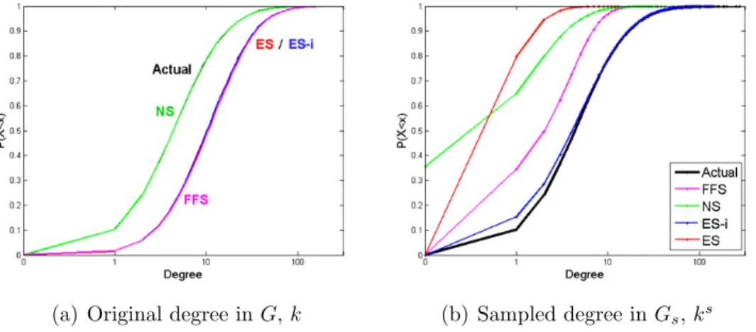
3.1 Illustration of Original versus Sampled Degrees . . . 43
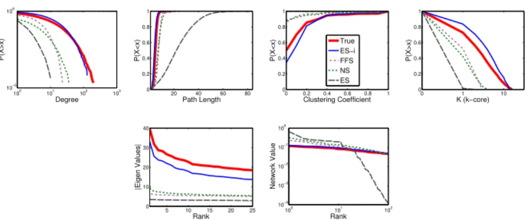
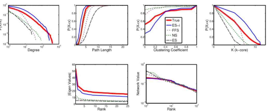
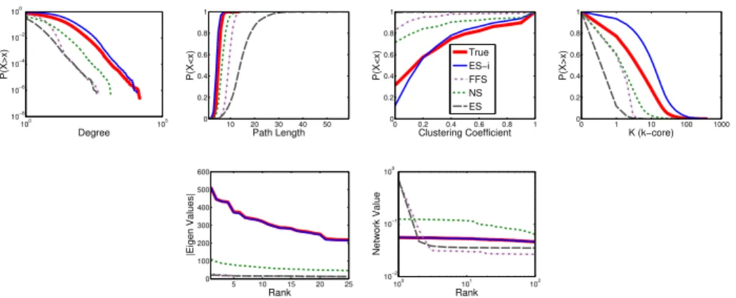
3.2 Average Distance Across Six Static Graphs. . . 46
3.3 Sampling Distribution of Facebook Graph . . . 49
3.4 Sampling Distribution of HepPH Graph . . . 49
3.5 Sampling Distribution of CondMAT Graph. . . 49
3.6 Sampling Distribution of Twitter Graph . . . 50
3.7 Sampling Distribution of Email-University Graph . . . 50
3.8 Sampling Distribution of Flickr Graph . . . 50
3.9 Sampling Distribution of LiveJournal Graph . . . 51
3.10 Estimation of Class Prior . . . 56
3.11 Classification Accuracy Versus Sampling Fraction . . . 58
3.12 Classification Accuracy Versus Proportion of Labeled Nodes . . . 59
4.1 Average Distance Across Six Streaming Graphs . . . 69
4.2 Stream Sampling Distribution of Pokec Graph . . . 71
4.3 Stream Sampling Distribution of Facebook Graph . . . 71
4.4 Stream Sampling Distribution of HepPH Graph . . . 72
4.5 Stream Sampling Distribution of CondMAT Graph . . . 72
4.6 Stream Sampling Distribution of Twitter Graph . . . 72
4.7 Stream Sampling Distribution of Email-Univ Graph . . . 73
4.8 Stream Sampling Distribution of Flickr Graph . . . 73
4.9 Stream Sampling Distribution of LiveJournal Graph . . . 73
Figure Page
4.11 Stream Sampling Distribution of Web-Stanford Graph . . . 74
4.12 Average KS Statistics for Dense and Sparse Graphs . . . 75
4.13 KS distance as a Function of Stream Length . . . 80
4.14 Distributions of Node Strength . . . 81
4.15 Distributions of Edge Weight . . . 81
4.16 Analysis of Node Strength Versus Node Degree . . . 83
4.17 Randomization Tests for Multigraph Streams . . . 84
5.1 Convergence Analysis of Graph Sample & Hold . . . 105
5.2 Analysis of Sample and Hold Probabilities . . . 109
6.1 4–node Motif Transition Diagram . . . 127
6.2 Illustration of Edge Neighborhood . . . 129
6.3 Runtime of Exact Motif Counting . . . 148
6.4 Anomaly Detection in Facebook University Networks . . . 150
ABSTRACT
Ahmed, Nesreen K. PhD, Purdue University, August 2015. Scaling Up Network
Analysis and Mining: Statistical Sampling, Estimation, and Pattern Discovery.
Major Professor: Jennifer Neville.
Network analysis and graph mining play a prominent role in providing insights and studying phenomena across various domains, including social, behavioral, biological, trans-portation, communication, and financial domains. Across all these domains, networks arise as a natural and rich representation for data. Studying these real-world networks is crucial for solving numerous problems that lead to high-impact applications. For example, iden-tifying the behavior and interests of users in online social networks (e.g., viral marketing), monitoring and detecting virus outbreaks in human contact networks, predicting protein functions in biological networks, and detecting anomalous behavior in computer networks. A key characteristic of these networks is that their complex structure is massive and con-tinuously evolving over time, which makes it challenging and computationally intensive to analyze, query, and model these networks in their entirety. In this dissertation, we propose sampling as well as fast, efficient, and scalable methods for network analysis and mining in both static and streaming graphs.
We develop a generic framework for statistical network stream sampling, called graph sample and hold. We formulate network sampling as a principled approach with two main functions: (1) the sampling function, and (2) the holding function, this approach allows tuning the sampling and estimation of graph properties more efficiently and accurately than the state-of-the-art. We develop a suite of algorithms to sample and estimate various graph properties, while processing the graph sequentially as a stream of edges. Finally, we develop a fast parallel algorithm for counting motifs, which is 460 times faster than the state-of-the-art. We show how these motif patterns can be used as features to benefit various machine learning tasks such as large-scale graph classification, prediction, anomaly detection, and visual analytics.
1. INTRODUCTION
Network analysis and graph mining play a prominent role in providing insights and studying phenomena across various domains, including social, behavioral, biological, transportation, communication, and financial domains. Across all these domains, networks arise as a natural and rich data representation. Studying these networks is crucial for solving numerous problems that lead to high-impact applications. For example, consider online activity and interaction networks formed from electronic communication (e.g., email, SMS, IMs), social media (e.g., Twitter, blogs, web pages), and content sharing (e.g., Facebook, Flicker, Youtube). These social tools produce a prolific amount of continuous and interaction data (e. g., Facebook users post 3.2 billion likes and comments every day [1]) that is naturally represented as a dynamic network—where the nodes are people or objects and the edges are the interactions among them.
Modeling and analyzing large dynamic networks have become increasingly im-portant for many applications. For example, identifying the behavior and interests of users in online social networks (e. g., viral marketing, online advertising) [2, 3], monitoring and detecting virus outbreaks in human contact networks [4], predict-ing protein functions in biological networks [5], and detectpredict-ing anomalous behavior in computer networks [6–8].
1.1 Challenges of Network Analysis and Mining
Many factors make it difficult and computationally intensive to study, analyze, query, or model these networks in their entirety [9–11]. First and foremost, the sheer size of many networks makes it computationally infeasible to study the entire network. Moreover, some networks are not completely visible to the public (e. g., Facebook),
can only be accessed through crawling (e. g., World Wide Web) [12], or their structure is dynamically changing over time (e. g., Twitter) [11, 13]. In other cases, the size of the full network may not be as large but the measurements required to observe the underlying network are costly (e. g., experiments in biological networks [14]). Thus, network sampling is at the heart and foundation of network analysis and mining— since researchers typically need to select a (tractable) subset of the nodes and edges from which to make inferences about the full network.
One key stumbling block for enabling large-scale graph analytics is the limitation in computational resources. Despite the recent advances in distributed and parallel processing frameworks for graph analytics (e.g. MapReduce), and the appearance of infinite resources in the cloud, running brute-force graph analytics is either too costly, too slow, or too inefficient in many practical situations [15–19]. This necessi-tates the development of fast, efficient, and approximation methods that exploit the characteristics of real-world networks to provide accurate, real-time analytics.
In many situations, finding an approximate answer is usually sufficient for many
types of analysis tasks, in which the extra cost and time in finding the exact answer
is often not worth the extra accuracy [20, 21]. In these cases, sampling provides an attractive approach to quickly and efficiently find an approximate answer to a query, or more generally, any graph analysis task.
Sampling has a long history for being efficient and useful to reduce storage re-quirements [22], speed up query execution times [23], and ensure data privacy by processing only a sample of the data from which to make inferences about the data population [24]. From peer-to-peer to social networks, sampling arises across many different settings [25–29]. For example, sampled networks may be used in simulations and experimentation—to measure performance before deploying new protocols and systems in the field, such as new Internet protocols, social/viral marketing schemes, A/B testing, and/or fraud detection algorithms.
Furthermore, many of the network data sets currently being analyzed as complete networks are themselves samples due to the above limitations in data collection [30,
31]. Thus, it is critical that researchers understand the impact of various sampling methods on the structure of the constructed networks. All of these factors motivate
the need for a more refined and complete understanding of network sampling.
Although a large body of research has developed methods to sample from net-works [25–29], much of the work is problem-specific, and there has been less work focused on developing a broader foundation for network sampling. More specifically, it is often not clear when and why particular sampling methods are appropriate. This is because the goals and population are often not explicitly defined or stated up front, which makes it difficult to evaluate the quality of the recovered samples for other applications. One of the primary aims of this work is to define the foun-dations of network sampling more explicitly, such as objectives/goals, population of interest, units, classes of sampling methods (i. e., node, edge, and topology-based), and techniques to evaluate a sample (e. g., network statistics and distance metrics).
In this chapter, we start in Section 1.2 by introducing a taxonomy for network sampling methods. Next, in Section 1.3, we highlight the key components and research questions that we address in this work. Finally, in Section 1.4, we summarize the main contributions and outline the structure of this dissertation.
1.2 A Taxonomy of Network Sampling Methods
Given a graph G= (V, E) as an input, how to sample a subgraph Gs= (Vs, Es)
with a subset of the nodes (Vs⊂V) and/or edges (Es⊂E) from the population graph
G? The goal is to ensure thatGsis representative, in the sense that graph properties
of interest are preserved in Gs (or can be estimated from Gs).
1.2.1 Classes of Network Sampling Methods
Network Sampling methods can be generally classified as node, edge, and topology-based sampling methods, topology-based on whether nodes or edges are first selected from the
more on the existing topology of G (topology-based sampling). More precisely, we define the three classes as follows:
• Node-based Sampling – Nodes are sampled with some probabilityp. For
ex-ample, in uniform node sampling, nodes are chosen independently and uniformly
at random from Gfor inclusion in the sampled subgraph Gs, and subsequently
edges that appear among these nodes are also added to Gs.
• Edge-based Sampling– Edges are sampled with some probability p. For
ex-ample, in uniform edge sampling, edges are chosen independently and uniformly
at random fromG for inclusion in the sampled subgraphGs.
• Topology-based Sampling – Nodes and edges in G are explored using some
variation of breadth-first search (i. e., sampling without replacement) or random walk (i. e., sampling with replacement) methods for inclusion in the sampled
subgraph Gs.
In the past years, most of the existing work has focused on studying topology-based sampling methods [9, 10, 26, 30, 32]. This trend was driven by the need of collecting data from the web (i. e., web crawling), and the limitations of applying node and edge-based sampling methods to collect data from distributed web and online social networks (e. g., Facebook),
1.2.2 Spectrum of Computational Models
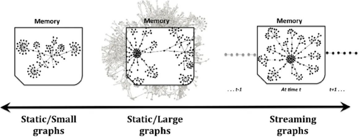
While most of the previous work focused on the question of how to sample, in
this dissertation, we discuss a spectrum of computational models for the design and implementation of network sampling methods. Then, we analyze sampling methods that generalize across this spectrum, going from the simplest and least constrained model focused on sampling from static graphs to the more difficult and most con-strained model of sampling from streaming graphs. This spectrum provides various opportunities for applying sampling methods in a variety of scenarios.
Static Network Sampling. Traditionally, network sampling has been studied in the case of simple static graphs [9,10,26,30,32]– such as forest fire, random walk and
snowball sampling methods. Given a disk-resident graph G, these works make the
simplifying assumption that the graph size is moderate and has a static structure. Specifically, it is assumed that the graph can fit entirely in the main memory, and the graph structure can be traversed arbitrarily (i. e., algorithms assume that the full neighborhood of each node can be accessed randomly in constant time), while many of the intrinsic complexities of realistic networks, such as the massive size, the time-evolving nature, and the temporal characteristics of these graphs, are totally ignored.
While studying static graphs is indeed important, the assumption that the graph fits in memory is not always realistic for real-world scenarios (e. g., online social networks). When the graph is too large to fit in memory, sampling requires random disk accesses that incur large I/O costs [33–35]. These random accesses on disks are typically much slower than random accesses in main memory [33]. Therefore, a key disadvantage of these methods is that they don’t differentiate between a graph that can fit entirely in the main memory and a graph that cannot. Naturally, this raises
the question: how can we sample from these large networks sequentially, one edge at
a time, while minimizing the number of passes over the edges? Given that the edges
can be stored in some arbitrary order, most of the topology-based sampling methods, such as breadth-first search, random walk, or forest-fire sampling, and node-based sampling methods are not appropriate as they require random access to a node’s neighbors (which would require many passes over the edges).
Streaming Network Sampling. In addition to their massive size, many
real-world networks are also likely to be continuously streaming over time. A streaming
graph is a rapid, continuous, and possibly unbounded, time-varying stream of edges
that is clearly too large to fit in memory except for short windows of time (e. g., a single day, hour, etc). Streaming graphs occur frequently in the real-world and can
Fig. 1.1.: Spectrum of Computational Models for network sampling: from static to streaming.
be found in many modern online and communication applications such as: Twitter posts, Facebook likes/comments, email communications, network monitoring, sensor networks, among many other applications [36]. Although these applications are quite prevalent, there has been little focus on developing network sampling algorithms that address the complexities of streaming graphs. Generally, streaming graphs differ from static graphs in four main aspects:
1. The massive volume of edges is far too large to fit into main memory
2. The graph structure is not fully observable at any point in time (i. e., only sequential access is feasible, not random access)
3. Efficient real-time processing is critically important
4. The stream exhibits temporal characteristics (e. g., edge frequency) that don’t appear in simple static graphs
Clearly, for such massive streaming graphs, sampling algorithms that process the
edge stream in single-pass and maintains a small consulting state in memory, are
These specific sampling algorithms are typically classified as graph stream sampling algorithms.
The above discussion shows a natural progression of computational models for network sampling—from static to streaming. The majority of previous work has focused on sampling from static graphs, which is the simplest and least restrictive problem setup. In this work, however, we investigate the more challenging issues of sampling from massive disk-resident and streaming graphs. This leads us to propose a spectrum of computational models for network sampling as shown in Figure 1.1, where we outline the computational models for sampling from: (1) static graphs, (2) large graphs, and (3) streaming graphs. This spectrum not only provides insights into the complexity of the computational models (i. e., static vs. streaming), but also the complexity of the algorithms that are designed for each scenario. More complex algorithms are more suitable for the simplest computational model of sampling from static graphs. In contrast, as the complexity of the computational model increases to a streaming scenario, efficient algorithms become necessary. Thus, there is a trade-off between the complexity of the sampling algorithm and the complexity of the
computational model (static → streaming).
A subtle but important consequence is that any algorithm designed to work over streaming graphs is also applicable in the simpler computational models (i. e., static graphs). However, the converse is not true, algorithms designed for sampling a static graph that can fit in memory, may not be generally applicable for streaming graphs (as their implementation may require an intractable number of passes over the data). Clearly, node and topology-based sampling methods are not efficient for sampling sequentially from the edge stream, on the other hand, edge-based sampling methods are naturally amenable to streaming implementation.
1.3 Problem Statement
From the previous discussion, it is clear that network sampling must mediate be-tween a variety of problem-specific constraints and opposing priorities [11, 37]. These constraints are defined by the problem under study, such as the characteristics of the data (e. g., heavy-tailed data distribution), the data access constraints (e. g., stream-ing vs. distributed data), the available resources (e. g., memory, bandwidth), and the accuracy needs of queries. In this dissertation, we propose network sampling methods that can mediate between a variety of problem-specific constraints. One of the
cen-tral questions in this dissertation is: given a graph G represented as an edge stream
{e1, e2, ..., et, ...}, how to sample a subgraphGs= (Vs, Es) sequentially, one edge at a
time, from the population graph G, while maintaining a small state |Ψ| ≤O(|Gs|)?
A key challenge for any stream sampling algorithm is the need to decide whether
to include an edgeet ∈E in the sample or not as the edge is observed in the stream.
The stream sampling algorithm may maintain a state |Ψ| and consult the state to
determine whether to sample an edge or not, but the total storage space (i. e., |Ψ|)
is usually of the order of the size of the output: |Ψ| = O(|Gs|). Note that this
requirement is potentially larger than the o(N) (and preferably polylog(N)) that
streaming algorithms typically require [35]. But since any algorithm cannot require less space than its output, we relax this requirement.
In this work, we propose a framework that can be used to design network sampling algorithms in the streaming computational model. Generally, the process of network sampling in the streaming computational model can be decomposed into two key functions: a (1) Sampling function, and a (2) Holding function. For each observed
edge et in the stream of edges {e1, e2, ..., et, ...}, the probability of selecting et can be
formulated as a conditional probability as follows,
If et is independent of the stored state Ψ, for example, et is not adjacent to
a previously selected edge, then (P[et is selected ] =PS), which means the selection
probability is a constant. We call this thesampling functionand we use it for sampling
and exploring new regions (unsampled) in the graph. On the other hand, if et is
not independent of the stored state Ψ, for example, et is adjacent to one or more
previously selected edges (ek ∈Ψ), then the selection probability is a function of the
stored (P[et is selected | stored state Ψ] =f(Ψ) , and PH =f(Ψ)). We call this the
holding functionand we use it for holding on or exploring a previously sampled region in the graph. This holding function essentially involves a frequent update of the state for each sampled edge. One of the primary challenges in this case is making sure the state updates do not cause state increase. In this work, we show ways for controlling the size of the sampled state, such as reservoir sampling [38] to ensure the size of the reservoir remains constant.
A key property of the proposed framework is that any edge-based sampling al-gorithm is statistically biased towards sampling graph regions that are much denser than the rest of the graph regions. This is due to the bias of edge-based sampling algorithms to the selection of high degree nodes and network hubs (see Chapter 3 for statistical bias analysis). It has been shown by Karger in [39] that edge-based sampling algorithms have a higher likelihood of containing graph cuts with lower value [40].
Moreover, the proposed framework is quite generic and flexible. By varying the conditional dependence of the sampling probabilities on the stored state, one can tune the estimation of various properties of the original graph efficiently with arbitrary degrees of accuracy. For example, in uniform edge sampling, the sampling probability of edges is a constant uniform probability and totally independent of the stored state. Thus, in the case of uniform edge sampling, the sampling and holding functions
are exactly the same, i. e., (P[et is selected ] =PS =PH =p). Furthermore, we can
adapt the holding function to simply track or capture certain graph properties (e. g., triangles). Similarly, by carefully designing the sampling function, we can obtain
a uniform random sample of nodes that appeared in the stream so far (similar to the classical uniform node sampling). Therefore, the proposed framework does not only help to design new sampling methods, but also to extend existing work to the streaming computational model.
The central thesis statement of this work is formulated as:
Statistical network stream sampling can be approached as a principled ap-proach with two main functions: (1) the sampling function, and (2) the holding function – By using this approach, we obtain a generic and flexi-ble framework that allows tuning the sampling and estimation of various graph properties efficiently and accurately, while being applicable across the full spectrum of computational models.
Throughout this dissertation, we investigate sampling as well as fast and efficient methods to scale up network analysis and mining in static and streaming graphs. We formally study two primary network analysis tasks: (1) Sampling a representative subgraph, and (2) Unbiased estimation and efficient methods for subgraph counting.
1.3.1 Sampling from Large Static Graphs
Given a large static disk-resident graph G= (V, E), the question of how to obtain
a representative subgraphGs= (Vs, Es) withn =|Vs|nodes fromGhas been studied
in previous work [9, 10, 26, 30, 32]. Most of the previous work assume that the graph
G can fit entirely in main
In this dissertation, we propose a two-pass sampling method that runs sequentially
with only two passes over the edge stream. The multi-pass computational model
takes a middle position in the memory spectrum by relaxing the polylog(N) storage
requirement of the streaming model [35, 41]. In addition to relaxing the memory requirement, the multi-pass model allows multiple passes over the input stream [35, 41]. In some applications, a small number of sequential passes over the edge stream
would be more efficient than many random disk accesses to the graph [41]. The proposed method is used to investigate three main research challenges:
• Given a large static disk-resident graph G, how can we sample fromG
sequen-tially, one edge at a time, while minimizing the number of passes over the edges?
• Analysis of the bias coming from sampling sequentially from the edge stream,
and the effect of the bias on the sampled subgraph.
• What is impact of different sampling methods on the performance of data
min-ing tasks, such as relational classification?
1.3.2 Sampling from Streaming Graphs
Today’s networks are not only large in size but also continuously streaming over time, and therefore, their structure can be viewed as a dynamical system. The normal operation of any dynamical system can be described by a process that transitions between different states over time. In this component, we study how to use network sampling to analyze the temporal and structural properties of streaming graphs.
Previous work has focused primarily on streaming uniform edge sampling, such as the work in [40], which is useful for some analysis tasks but not all of them. Therefore, we propose methods that extend traditional sampling algorithms from the various classes (e. g., node, edge, etc) into the streaming computational model. Then, We propose a novel graph stream sampling method that efficiently sample from the graph stream in a single pass. We evaluate these methods on a variety of multigraph streams and show their performance on both temporal and structural properties. Our work in this part is focused on exploring two main research challenges:
• Given a streaming graph et ∈ E, how to sample a representative subgraph in
a single-pass over the edge stream, while maintaining a small state in memory |Ψ| ≤O(|S|)?
• How to extend traditional sampling algorithms to streaming implementation in a single pass?
• What is the impact of single-pass stream sampling on structural and temporal
graph properties?
1.3.3 Big Graph Analytics and Unbiased Estimation
In this part, we focus on exploring fast, efficient approximation and exact methods to obtain counts of frequent patterns/subgraphs in the edge stream of the graph. One goal of this part is to develop methods useful for answering various graph queries accurately, quickly, and efficiently. For this goal, we propose a generic stream sampling framework for big graph analytics, called Graph Sample and Hold (gSH). gSH is a parametric framework that can be used to estimate subgraph counts, such as the number of edges, triangles, etc.
While previous work focused particularly on sampling schemes used to estimate a certain graph property [17, 19, 42–44], gSH is generic and can be used to estimate various graph properties with the same sampling scheme. Our framework starts by sampling from massive graphs sequentially in a single pass, one edge at a time, while maintaining a small state in memory. We also develop statistical estimators based on the construction of Horvitz-Thompson [45], and we apply them to obtain unbiased estimates of subgraph counts.
Another goal of this part is to extract useful structural features, such as motif frequencies, that would benefit important machine learning tasks. For example, large-scale graph classification, prediction, anomaly detection, among others. For this goal, we propose a fast efficient algorithm for motif counting that take only a fraction of the time to compute when compared with the current methods used. The proposed motif counting algorithm leverages a number of combinatorial arguments that we show for the different motif patterns. For each edge, we count a few of the patterns, and with these counts along with combinatorial arguments, we derive the exact counts of the
others in constant time. The combinatorial arguments we show enable us to obtain significant improvement on the scalability of motif counting.
In summary, we investigate the following research questions:
• How to quickly and efficiently estimate various subgraph counts, such as the
number of edges, triangles, etc?
• How to efficiently count all possible motifs (or graphlets) of size k = {2,3,4}
nodes?
1.4 Contributions and Outline
This dissertation is positioned to extend the range, applicability, and performance gains of network sampling as a tool that is not only useful for web crawling and data collection, but also for the analysis and mining of massive disk-resident and streaming graphs efficiently. We show how network sampling can be used as a mediator of various problem-specific constraints, such as the characteristics of the data (e. g., heavy-tailed data distribution), the data access constraints (e. g., streaming vs. distributed data), the available resources (e. g., memory, bandwidth), and the accuracy needs of queries. We propose a flexible framework for designing statistical graph stream sampling. The potential benefits of the proposed framework are two-fold. First, it will lead to more interpretable sampling designs, that efficiently capture the specific graph properties of interest. This should benefit big graph analytics and data mining ap-plications in general, since interpretability is a quality that is often important for domain experts to design useful sampling methods. Second, it will lead to samples with better quality that efficiently mirror the properties of the population graph.
In addition, we propose a fast efficient algorithm for motif counting that is sig-nificantly faster than the current methods used, while also scaling to much larger networks with millions of nodes and edges. The proposed motif counting algorithm leverages a number of combinatorial arguments, which enable us to obtain significant improvement on the scalability of motif counting. Thus, this brings new
opportu-nities to investigate the use of motifs on much larger networks and newer applica-tions. Furthermore, a number of important machine learning applications are likely to benefit from such algorithm, including graph-based anomaly detection [7, 46], en-tity resolution [47], as well as features for improving community detection [48], role discovery [49], and relational classification [50, 51].
The rest of this dissertation is organized as follows: Chapter 2 describes the foundations of network analysis and sampling, highlighting the different objectives of network sampling, the population and units with respect to the specific goals, evaluation and classes of network sampling methods. In Chapter 3, we introduce our approach to sampling a subgraph from large static graphs. Next, in Chapter 4, we introduce our approach to sampling from streaming graphs. Then, we describe our framework for unbiased estimation of counts of frequent subgraphs in Chapter 5. In Chapter 6, we introduce our fast efficient algorithm for motif counting (counting all
possible subgraphs of size 2,3,4 nodes). Finally, Chapter 7 concludes the dissertation
and points out for future directions.
Parts of this dissertation have been published in peer-reviewed conferences and journals. In particular, the work in Chapter 2 and Chapter 3 is published in the ACM journal of TKDD [11] and WIN [52]. Parts of the work in Chapter 3 is published in ICWSM [53], and MLG [54]. Also, the work in Chapter 4 is published in the ACM journal of TKDD [11] and BigMine [55]. Moreover, the work in Chapter 5 is published in SIGKDD [23]. Finally, the work in Chapter 6 is published in [56], and other parts of this chapter are published in ICWSM [57].
2. BACKGROUND
In the context of statistical data analysis, a number of issues need to be considered carefully before collecting data and making inferences based on them. First, we need
to identify the relevant populationto be studied. Then, if sampling is necessary then
we need to decide how to sample from that population. Generally, the termpopulation
is defined as the full set of representative units that one wishes to study (e. g., individ-uals in a particular city). In some instances, the population may be relatively small and therefore easy to study in its entirety (i. e., without sampling). For instance, it is
fairly easy to study the fullset of graduate students in a particular academic
depart-ment. However, in many situations the population is large, unbounded, or difficult and/or costly to access in its entirety (e. g., the complete set of Facebook users). In this case, for efficiency reasons, a sample of units can be collected and characteristics of the population can then be estimated from the sampled units.
Network sampling is of interest to a variety of researchers in a range of distinct fields (e. g.statistics, social science, databases, data mining, machine learning) due to the numerous complex data sets that can be represented as graphs. While each
area may investigate different types of networks, they have all considered how to
sample. For example, in social science, snowball sampling is used extensively to run survey sampling in populations that are difficult-to-access (e. g., the set of drug users in a city) [58]. Similarly, in Internet topology measurements, breadth first search is
used to crawl distributed, large-scale online social networks [30]. In structured data
mining and machine learning, the focus has been on developing algorithms to sample small(er) subgraphs from a single large network [9]. These sampled subgraphs are further used to learn models (e. g., relational classification models [59]), evaluate and compare the performance of algorithms (e. g., different classification methods [60,61]),
and study complex network processes (e. g., information diffusion [62]). Section 2.6 provides a more detailed discussion of related work.
While this large body of research has developed methods to sample from networks, much of the work is problem-specific and there has been less work focused on devel-oping a broader foundation for network sampling. More specifically, it is often not
clear when and why particularly sampling methods are appropriate. This is because
the goals and population are often not explicitly defined or stated up front, which makes it difficult to evaluate the quality of the recovered samples for other applica-tions. One of the primary aims of this work is to define and discuss the foundations of network sampling more explicitly, such as: objectives/goals, population of inter-est, units, classes of sampling algorithms (i. e., node, edge, and topology-based), and techniques to evaluate a sample (e. g., network statistics and distance metrics). In this chapter, we outline a solid methodological framework for network sampling. The framework will facilitate the comparison of various network sampling algorithms, and help to understand their relative strengths and weaknesses with respect to particular sampling goals.
2.1 Foundations and Notations
Formally, we consider an input network represented as a graph G= (V, E) with
the node set V ={v1, v2, ..., vN}and edge setE ={e1, e2, ..., eM}, such thatN =|V|
is the number of nodes, andM =|E| is the number of edges. We denote η(.) as any
topological graph property. Therefore, η(G) could be a point statistic (e. g., average
degree of nodes inV) or a distribution(e. g., degree distribution of V inG).
Further, we define Λ ={a1, a2, ..., ak}as the set ofk attributes associated with the
nodes describing their properties. Each node vi ∈V is associated with an attribute
vector [a1(vi), a2(vi), ..., ak(vi)] where aj(vi) is the jth attribute value of node vi. For
friendships, the node attributes may include age, political view, and relationship status of the user.
Similarly, we denoteβ ={b1, b2, ..., bl}as the set oflattributes associated with the
edges describing their properties. Each edge eij = (vi, vj) ∈ E is associated with an
attribute vector [b1(eij), b2(eij), ..., bl(eij)]. In the Facebook example, edge attributes
may include relationship type (e. g., friends, married), relationship strength, and type of communication (e. g., wall post, photo tag).
Now, we define the network sampling process. Let σ be any sampling algorithm
that selects a random sampleS fromG(i. e.,S =σ(G)). The sampled setS could be
a subset of the nodes (S =Vs⊂V) , or edges (S =Es⊂E), or a subgraph (S= (Vs, Es)
where Vs⊂V and Es⊂E). The size of the sample S is defined relative to the graph
size with respect to a sampling fractionφ (0≤φ≤1). In most cases the sample size
is defined as a fraction of the nodes in the input graph, e. g., |S| = φ· |V|. But in
some cases, the sample size is defined relative to the number of edges (|S|=φ· |E|).
2.2 Goals, Units, and Population of Networks
While the explicit aim of many network sampling algorithms is to select a smaller
subgraph fromG, there are often other more implicit goals of the process that are left
unstated. Here, we formally outline a range of possible goals for network sampling:
(Goal 1) Estimate network parameters
Let S ⊂ V or S ⊂ E. Then for a property η of G, if η(S) ≈ η(G), S is
considered a good sample ofG.
For example, let S = Vs ⊂ V be the subset of sampled nodes, we can
estimate the average degree of nodes G usingS:
d degavg = 1 |S| X vi∈S deg(vi ∈G)
where deg(vi ∈G) is the degree of node vi as it appears in G, and a direct
application of statistical estimators helps to correct sampling bias inddegavg
[63].
(Goal 2) Sample a representative subgraph
Let S=Gs refer to a subgraph Gs= (Vs, Es) sampled from G. Then for a
set of topological properties ηA of G, if ηA(S) ≈ ηA(G), S is considered a
good sample of G.
Generally, subgraph representativeness is evaluated by selecting a set of graph topological properties that are important for a wide range of
appli-cations. This ensures that the sample subgraph S can be used in place of
Gfor testing algorithms, systems, and/or models in an application. For
ex-ample, [9] evaluated sample quality using topological properties like degree, clustering, and eigenvalues.
(Goal 3) Estimate node attributes
LetS ⊂V. Then for a function fa of node attribute a, iffa(S)≈fa(V),S
is considered a good sample ofV (where V is the set of nodes in G).
For example, if a represents the age of users, we can estimate the average
in Gusing S: baavg = 1 |S| X vi∈S a(vi)
Similar to goal 1, statistical estimators can be used to correct for bias.
(Goal 4) Estimate edge attributes
Let S ⊂ E. Then for a functionfb of edge attribute b, if fb(S)≈ fb(E), S
For example, if b represents the relationship type of friends (e. g., married,
coworkers), we can estimate the proportion of married relationships in G
using S: b pmarried = 1 |S| X eij∈S 1(b(eij)=married)
Clearly, the first two goals (1 and 2) focus on characteristics of entire networks, while the last two goals (3 and 4) focus on characteristics of nodes or edges in isolation. Therefore, these goals may be difficult to satisfy simultaneously—i.e., if the sampled data enable accurate study for one, it may not allow accurate study for others. For instance, a representative subgraph sample could produce a biased estimate of node attributes.
Once the goal is outlined, the population of interest can be defined relative to the goal. In many cases, the definition of the population may be obvious (e. g., nodes in the network). The main challenge is then to select a representative subset of units in the population in order to make the study cost efficient and feasible. Other times, the population may be less tangible and difficult to define. For example, if one wishes
to study the characteristics of a system orprocess, there is not a clearly defined set of
items to study. Instead, one is often interested in the overall behavior of the system. In this case, the population can be defined as the set of possible outcomes from
the system (e.g., measurements over all settings) and these unitsshould be sampled
according to their underlying probability distribution.
In the first two goals outlined above, the objective of study is an entire network (either for structure or parameter estimation). In goal 1, if the objective is to estimate
local properties from the nodes (e. g.degree distribution of G), then the elementary
units are the nodes, and then the population would be the set of all nodes V in G.
However, if the objective is to estimate global properties (e. g.diameter of G), then
the elementary units correspond to subgraphs (any Gs ⊂ G) rather than nodes and
could be drawn fromG. In goal 2, the objective is to select a subgraph Gs, thus the
elementary units correspond to subgraphs, rather than nodes or edges (goal 3 and 4). As such, the population should also be defined as the set of subgraphs of a particular
size that could be drawn from G.
2.3 Classes of Sampling Methods
Once the population has been defined, a sampling algorithm σ must be chosen to
sample fromG. Sampling algorithms can be categorized as node, edge, and
topology-based sampling, topology-based on whether nodes or edges are locally selected from G (node
and edge-based sampling) or if the selection of nodes and edges depends more on the
existing topology of G (topology-based sampling).
Graph sampling algorithms have two basic steps:
(1) Node selection: used to sample a subset of nodes S =Vs from G, (i. e., Vs ⊂V).
(2) Edge selection: used to sample a subset of edgesS =Es from G, (i. e.,Es ⊂E)
When the objective is to sample only nodes or edges (e. g., goals 3,4 or 1), then
either step 1 or step 2 is used to form the sampleS. When the objective is to sample
a subgraphGs fromG(e. g., goals 2 or 1), then both step 1 and 2 from above are used
to form S, (i. e., S= (Vs, Es)). In this case, the edge selection is often conditioned
on the selected node set in order to form an induced subgraph by sampling a subset
of the edges incident to Vs (i. e.Es = {eij = (vi, vj)|eij ∈ E ∧ vi, vj ∈ Vs}. This
process is called graph induction. We distinguish between two approaches of graph
induction—totaland partial graph induction—which differ by whether all orsomeof
the edges incident on Vs are selected. The resulting sampled graphs are referred to
as the induced subgraphand partially induced subgraph respectively.
While the discussion of the algorithms in the next chapters focuses more on
sam-pling a subgraph Gs from G, they can easily generalize to sampling only nodes or
Node sampling (NS). In classic node sampling, nodes are chosen independently
and uniformly at random fromGfor inclusion in the sampled graphGs. For a target
fraction φ of nodes required, each node is simply sampled with a probability of φ.
Once the nodes are selected for Vs, the sampled subgraph is constructed to be the
induced subgraph over the nodes Vs, i. e., all edges among the Vs ∈ G are added to
Es. While node sampling is intuitive and relatively straightforward, the work in [64]
shows that it does not accurately capture properties of graphs with power-law degree distributions. Similarly, [65] shows that although node sampling appears to capture nodes of different degrees well, due to its inclusion of all edges for a chosen node set only, the original level of connectivity is not likely to be preserved.
Edge sampling (ES). In classic edge sampling, edges are chosen independently
and uniformly at random from G for inclusion in the sampled graph Gs. Since edge
sampling focuses on the selection of edges rather than nodes to populate the sample,
the node set is constructed by including both incident nodes in Vs when a particular
edge is sampled (and added to Es). The resulting subgraph is partially induced,
which means no extra edges are added over and above those that were chosen during the random edge selection process. Unfortunately, ES fails to preserve many desired graph properties. Due to the independent sampling of edges, it does not preserve clustering and connectivity. It is however more likely to capture path lengths, due to its bias towards high degree nodes and the inclusion of both end points of selected edges.
Topology-based sampling. Due to the known limitations of NS [64, 65] and ES
(bias toward high degree nodes), researchers have also considered many other topology-based sampling methods (also referred to as exploration sampling), which use breadth-first search (i. e., sampling without replacement) or random walks (i. e., sampling with replacement) over the graph to construct a sample.
One example is snowball sampling, which adds nodes and edges using breadth-first search from a randomly selected seed node, but stops early once it reaches a
particular size. Snowball sampling accurately maintains the network connectivity
within the snowball, but it suffers from boundary bias in that many peripheral nodes
(i. e., those sampled on the last round) will be missing a large number of neighbors [65].
Another example is the Forest Fire Sampling (FFS) method [9], which usespartial
breadth-first search where only a fraction of neighbors are followed for each node. The algorithm starts by picking a node uniformly at random and adding it to the sample. It then “burns” a random proportion of its outgoing links, and adds those edges, along with the incident nodes, to the sample. The fraction is determined by sampling from
a geometric distribution with mean (pf/(1−pf)). The authors recommend setting
pf = 0.7, which results in an average burn of 2.33 edges per node. The process is
repeated recursively for each burned neighbor until no new node is selected, then a new random node is chosen to continue the process until the desired sample size is obtained. There are other algorithms such as respondent-driven sampling [66] and expansion sampling [28] that we give more details on in Chapter 2.6.
In general, such topology-based sampling approaches form the sampled graph out of the explored nodes and edges, and usually perform better than simple algorithms such as NS and ES.
2.4 Evaluation of Sampling Methods
When the goal is to approximate the entire input network—either for estimating parameters (goal 1) or to select a representative subgraph structure (goal 2)—the accuracy of network sampling methods is often measured by comparing structural network statistics (e. g., degree). We first define a suite of common network statistics and then discuss how they can be used to quantitatively compare sampling methods.
Network Statistics. The commonly considered network statistics can be compared
along two dimensions: local vs. global statistics, and point statistic vs. distribution.
A local statistic is is used to describe a characteristic of a local graph element (e. g., node, edge, subgraph). For example, node degree and node clustering coefficient.
Table 2.1.: Description of Network Statistics
Network Statistic. Description
Degree dist. Distribution of degrees for all nodes in the network
Path length dist. Distribution of (finite) shortest path lengths between all pairs of nodes in the network
Clustering coefficient dist. Distribution of local clustering for all nodes in the network
K-core dist. Distribution ofk-core decomposition of the network
Eigenvalues Distribution of the eigenvalues of the network adja-cency matrix vs. their rank
Network values Distribution of eigenvector components vs. their rank, for the largest eigenvalue of the network ad-jacency matrix
On the other hand, a global statistic is used to describe a characteristic of the entire graph. For example, global clustering coefficient and graph diameter. Similarly, there is also the distinction between point statistics and distributions. A point-statistic is a single value statistic (e. g., diameter) while a distribution is a multi-valued statistic (e. g., distribution of path length for all pairs of nodes). Clearly, a range of network statistics are important to investigate the full graph structure.
In this work, we focus on the goal of sampling a representative subgraph Gs from
G, by using distributions of network characteristics calculated on the level of nodes,
edges, sets of nodes or edges, and subgraphs. Table 2.1 provides a summary for the six network statistics we use and we formally define the statistics below:
(1) Degree distribution: The fraction of nodes with degreek, for all k >0
pk = |{v∈V|degN(v)=k}|
Degree distribution has been widely studied by many researchers to understand the connectivity in graphs. Many real-world networks were shown to have a
power-law degree distribution, for example in the Web [67], citation graphs [68], and online social networks [69].
(2) Path length distribution: Also known as thehop plotdistribution and denotes the
fraction of pairs (u, v)∈V with a shortest-path distance (dist(u, v)) of h, for all
h >0 and h6=∞
ph = |{(u,v)∈V|Ndist2 (u,v)=h}|
The path length distribution is essential to know how the number of paths between nodes expands as a function of distance (i. e., number of hops).
(3) Clustering coefficient distribution: The fraction of nodes with clustering
coeffi-cient (cc(v)) c, for all 0≤c≤1
pc= |{v∈V
0|cc(v)=c}|
|V0| , whereV0 ={v ∈V|deg(v)>1}
Here the clustering coefficient of a node v is calculated as the number of triangles
centered onvdivided by the number of pairs of neighbors ofv(e. g., the proportion
ofv’s neighbor that are linked). In social networks and many other real networks,
nodes tend to cluster. Thus, the clustering coefficient is an important measure to capture the transitivity of the graph [70].
(4) K-core distribution: The fraction of nodes in graphG participating in ak-coreof
order k. The k-core of G is the largest induced subgraph with minimum degree
k. Formally, letU ⊆V, and G[U]= (U, E0) whereE0={eu,v ∈E|u, v ∈U}. Then
G[U] is a k-core of order k if ∀v∈U degG[U](v)≥k.
Studyingk-coresis an essential part of social network analysis as they demonstrate
the connectivity and community structure of the graph [71–73]. We denote the
maximum core numberas the maximum value of kin thek-coredistribution. The
maximum core number can be used as a lower bound on the degree of the nodes
that participate in the largest induced subgraph ofG. Also, the core sizes can be
(5) Eigenvalues: Let A be the corresponding adjacency matrix of a graph G, then
the decomposition of A into eigenvalues (Λ = [λ1, ..., λn]) and eigenvectors (X =
[X1, ..., Xn]) satisfies the equation (A−λI)X = 0, where I is the NxN identity
matrix. We number the set of eigenvalues (and associated eigenvectors) in
de-scending order λ1 ≥...≥ λN, then we compare the largest 25 eigenvalues of the
sampled graphs to their counterparts in G. Note that eigenvalues are the basis
of spectral graph analysis [75].
(6) Network values: The distribution of the principal eigenvector components (i. e.,
the components xi ∈ X1 associated with the largest eigenvalue λ1 of the graph
adjacency matrix). We compare the largest 100 components of the principal
eigenvector of the sampled graphs to their counterparts in G.
Next, we describe the use of these statistics for comparing sampling methods.
Distance Measures for Quantitatively Comparing Sampling Methods. A
good sample has properties that approximate the full graph G (i.e., η(S) ≈ η(G)).
Thus, the distance between the property inGand the property inGsis often used to
evaluate sample representativeness quantitatively (i. e., dist[η(G), η(GS)]) and
sam-pling algorithms that minimize the distance are considered superior. When the goal
is to provide estimates of global network parameters (e. g., average degree), thenη(.)
may return point statistics. However, when the goal is to provide a representative
subgraph sample, then η(.) may return distributionsof network properties (e. g.,
de-gree distribution). These distributions reflect how the graph structure is distributed
across nodes and edges. Thedist function used for evaluation could be typically any
distance measure (e. g., absolute difference). In this chapter, since we focus on us-ing distributions to characterize graph structure, we use four different distributional distance measures for evaluation.
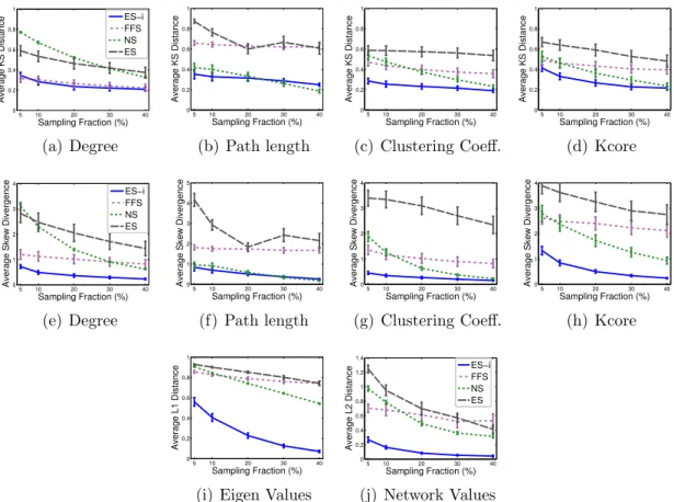
(1) Kolmogorov-Smirnov (KS) statistic: Used to assess the distance between two cumulative distribution functions (CDF). The KS-statistic is a widely used mea-sure of the agreement between two distributions, including in [9] where it is used
to illustrate the accuracy of FFS. It is computed as the maximum vertical
dis-tance between the two distributions, wherex represents the range of the random
variable and F1 and F2 represent two CDFs:
KS(F1, F2) =maxx|F1(x)−F2(x)|
(2) Skew divergence (SD): Used to assess the difference between two probability den-sity functions (PDF) [76]. Skew divergence is used to measure the
Kullback-Leibler (KL) divergence between two PDFs P1 and P2 that do not have
contin-uous support over the full range of values (e. g., discrete degrees). KL measures the average number of extra bits required to represent samples from the original distribution when using the sampled distribution. However, since KL divergence is not defined for distributions with different areas of support, skew divergence
smoothsthe two PDFs before computing the KL divergence:
SD(P1, P2, α) =KL[αP1+ (1−α)P2||αP2+ (1−α)P1]
The results shown in [76] indicate that using SD yields better results than other methods to approximate KL divergence on non-smoothed distributions. In this
work, as in [76], we use α = 0.99.
(3) Normalized L1 distance: In some cases, for evaluation we will need to measure
the distance between two positive m-dimensional real vectors p and q such that
p is the true vector and q is the estimated vector. For example, to compute the
distance between two vectors of eigenvalues. In this case, we use the normalized
L1 distance:
L1(p, q) = m1 Pmi=1 |
pi−qi| pi
(4) NormalizedL2 distance: In other cases, when the vector components are fractions
(less than one), we use the normalized euclidean distance L2 distance (e. g., to
compute the distance between two vectors of network values):
2.5 Models of Computation
In this section, we discuss the different models of computation that can be used to
implement network sampling methods. At first, let us assume the networkG= (V, E)
is given (e. g., stored on a large storage device). Then, the goal is to select a sample
S fromG.
Traditionally, network sampling has been explored in the context of a static model
of computation. This simple model makes the fundamental assumption that it is easy
and fast (i. e., constant time) to randomly access any location of the graph G. For
example, random access may be used to query the entire set of nodesV or to query the
neighbors N(vi) of a particular node vi (where N(vi) ={vj ∈V|eij= (vi, vj)∈E}).
However, random accesses on disks are much slower than random accesses in main memory. A key disadvantage of the static model of computation is that it does not differentiate between a graph that can fit entirely in the main memory and a graph that cannot. Conversely, the primary advantage of the static model is that it is a
natural extension of how we understand and view the graph—thus, it is a simple
framework within which to design algorithms.
Although designing sampling algorithms with a static model of computation in mind is indeed appropriate for some applications, this approach assumes the input graphs are relatively small, can fit entirely into main memory, and have static struc-ture (i. e., not changing over the time). This is unrealistic for many domains. For instance, many social, communication, and information networks naturally change over time and are massive in size (e. g., Facebook, Twitter, Flickr). The sheer size and dynamic nature of these networks make it difficult to load the full graph entirely in the main memory. Therefore, the static model of computation cannot realistically capture all the intricacies of many real world graphs that we study today.
In addition, many real-world networks that are currently of interest are too large
to fit into memory. In this case, sampling methods that require random disk access can incur large I/O costs for loading and reading the data. Naturally, this raises
a question as to how we can sample from large networks more efficiently (i.e., in a sequential fashion rather than assuming random access). In this context, most of the topology based sampling procedures such as breadth-first search and random-walk sampling are no longer appropriate as they require the ability to randomly access a
node’s neighbors N(vi). If access is restricted to sequential passes over the edges, a
large number of passes over the edges would be needed to repeatedly queryN(·). In
a similar way, node sampling would no longer be appropriate as it not only requires random access for querying a node’s neighbors but it also requires random access to
the entire node setV in order to obtain a uniform random sample.
A streaming model of computation in which the graph can only be accessed se-quentially as a stream of edges, is therefore more preferable for these situations [77].
The streaming model completely discards the possibility of random access to G and
the graph can only be accessed through an ordered scan of the edge stream. A sam-pling algorithm in this context may use the main memory for holding a portion of the edges temporarily and perform random accesses on that subset. In addition, the sampling algorithm may access the edges repeatedly by making multiple passes over
the graph stream. Formally, for any input network G, we assumeGis represented as
a graph stream (e.g., as in Figure 2.1).
Definition 2.5.1 (Graph Stream) Agraph stream is an ordered sequence of edges
eπ(1), eπ(2), ..., eπ(M), where π is any arbitrary permutation on the edge indices [M] = {1,2, ..., M}, π : [M]→[M].
Definition 2.5.1 is usually called the “adjacency stream” model in which the graph is presented as a stream of edges in an arbitrary order. In contrast, the “incidence stream” model assumes all edges incident to a vertex are presented in order suc-cessively [43]. In this work, we use the adjacency stream model because it is more reflective of the temporal ordering we observe in real world data sets.
While most real-world networks are too large to fit into main memory, many are