Learning to Rank Algorithms and their Application in Machine Translation

(1)

Wright State University Wright State University

CORE Scholar

Browse all Theses and Dissertations Theses and Dissertations

2015

Learning to Rank Algorithms and their Application in Machine

Translation

Tian Xia

Wright State University

Follow this and additional works at: https://corescholar.libraries.wright.edu/etd_all

Part of the Computer Engineering Commons, and the Computer Sciences Commons

Repository Citation Repository Citation

Xia, Tian, "Learning to Rank Algorithms and their Application in Machine Translation" (2015). Browse all Theses and Dissertations. 1643.

https://corescholar.libraries.wright.edu/etd_all/1643

(2)

Learning to Rank Algorithms and Their

Application in Machine Translation

A thesis submitted in partial fulfillment

of the requirements for the degree of

Doctor of Philosophy

by

Tian Xia

M.S., Chinese Academy of Sciences, 2011

B.S., Xidian University, 2007

2015

(3)

Wright State University GRADUATE SCHOOL

November 12, 2015 I HEREBY RECOMMEND THAT THE THESIS PREPARED UNDER MY SUPER-VISION BY Tian Xia ENTITLED Learning to Rank Algorithms and Their Application in Machine Translation BE ACCEPTED IN PARTIAL FULFILLMENT OF THE RE-QUIREMENTS FOR THE DEGREE OF Doctor of Philosophy.

Shaojun Wang, Ph.D. Dissertation Director

Michael Raymer, Ph.D. Director, Department of Computer Science and Engineering

Robert E. W. Fyffe, Ph.D. Vice President for Research and Dean of the Graduate School Committee on Final Examination

Keke Chen, Ph.D.

Xinhui Zhang, Ph.D.

(4)

ABSTRACT

Xia, Tian. Ph.D., Department of Computer Science and Engineering, Wright State University, 2015.Learning to Rank Algorithms and Their Application in Machine Translation.

In this thesis, we discuss two issues in the learning to rank area, choosing effective objective loss function, constructing effective regresstion trees in the gradient boosting framework, as well as a third issus, applying learning to rank models into statistcal ma-chine translation.

First, list-wise based learning to rank methods either directly optimize performance measures or optimize surrogate functions of performance measures that have smaller gaps between optimized losses and performance measures, thus it is generally believed that they should be able to lead to better performance than point- and pair-wise based learning to rank methods. However, in real-world applications, state-of-the-art practical learning to rank systems, such as MART and LambdaMART, are not from list-wise based camp. One cause may be that several list-wise based methods work well in the popular but very small LETOR datasets but fail in real-world datasets that are often used for training practical systems.

We propose a list-wise learning to rank method that is based on a list-wise surrogate function, the Plackett-Luce (PL) model. The PL model has convex loss to ensure a global optimal guarantee, and is proven to be consistent to certain performance measures such as NDCG score. When we conduct experiments on the PL model, we observe that it is actually unstable in performance; when the data has rich enough features, it gives very good results, but for data with scarce features, it fails horribly. For example, when we

(5)

apply the PL with a linear model on the Microsoft 30K dataset, it gives 7.6 points worse NDCG@1 score than an average performance of several linear systems. This motivates us to propose our new ranking system, PLRank, that is suitable for any data sets through a mapping from feature space into tree space to gain more expressive power. PLRank is trained based on the gradient boosting framework, and it is simple to implement. It has the same time complexity as the LambdaMART, and runs a little bit faster in practice. More-over, we extend three other list-wise surrogate functions in a gradient boosting framework for a fair and full comparison, and we find that the PL model has special advantages.

Our experiments are conducted on the two largest publicly available real-world datasets, Yahoo challenge 2010 and Microsoft 30K. The results show this is the first time in the sin-gle model level for a list-wise based system to match or overpass state-of-the-art point-and pair-wise based ones, MART, LambdaMART, point-and McRank, in real-world datasets.

Second, industry-level applications of learning to rank models have been dominated by gradient boosting framework, which fits a tree using least square error (SE) principle. An-other tree fitting principle, (robust) weighted least square error ((R)WSE), has been widely used in classification, such as LogitBoost and its variants, but hasn’t been reformulated to fulfill learning the rank tasks. For both principles, there is a lack of deep analysis on their relationship in the scenario of learning to rank. Motivated by AdaBoost, we propose a new principle named least objective loss based error (OLE) that enables us to analyze sev-eral important learning to rank systems:we prove that (R)WSE is actually a special case of OLE for derivative additive loss functions; OLE, (R)WSE and SE are equivalent for MART system. Under the guidance of OLE principle, we implement three typical and strong sys-tems and conduct our experiments in two real-world datasets. Experimental results show

(6)

that our proposed OLE principle improves most results over SE.

Thrid, Margin infused relaxed algorithms (MIRAs) dominate model tuning in statis-tical machine translation in the case of large scale features, but also they are famous for the complexity in implementation. We introduce a new method, which regards an N-best list as a permutation and minimizes the Plackett-Luce loss of ground-truth permutations. Experiments with large-scale features demonstrate that, the new method is more robust than MERT ; though it is only matchable with MIRAs, it has a comparatively advantage, easier to implement.

(7)

3.1.3 (R)WSE⊂OLE . . . 50

3.1.4 SE = (R)WSE = OLE for MART . . . 51

3.2 Experiments . . . 54

3.2.1 Datasets and Systems . . . 54

3.2.2 Experimental Comparison with Three Systems . . . 60

4 A Simple Discriminative Training Method for Machine Translation with Large-Scale Features 72 4.1 Plackett-Luce Model . . . 72

4.2 Plackett-Luce Model in Statistical Machine Translation . . . 74

4.3 Evaluation . . . 77

4.3.1 Plackett-Luce Model for SMT Tuning . . . 78

4.3.2 Plackett-Luce Model for SMT Reranking . . . 80

5 Conclusion 82

(9)

List of Figures

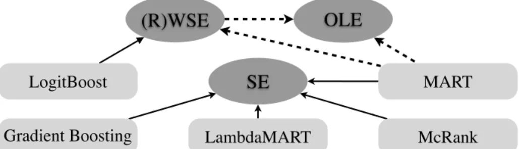
1.1 Three node splitting principles in decision tree construction, namely Square Error (SE) in Gradient Boosting framework, Robust Weighted Square Er-ror (RWSE) in the LogitBoost system, and Objective Loss Based ErEr-ror (OLE) in this paper, as well as their relations. All real-line arrows denote known relations, and dotted-line arrows denote our contribution. . . 13

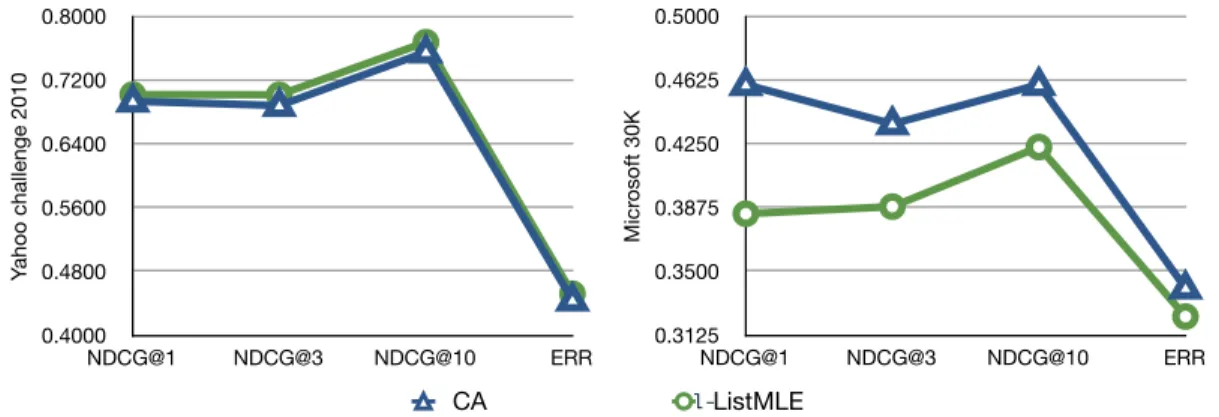
2.1 The performance of l-ListMLE and the selected linear reference system

Coordinate Ascent (CA) on Yahoo data (left) and Microsoft 30K (right). CA is capable of representing the mainstream linear systems on these datasets Tan et al. (2013a). . . 33

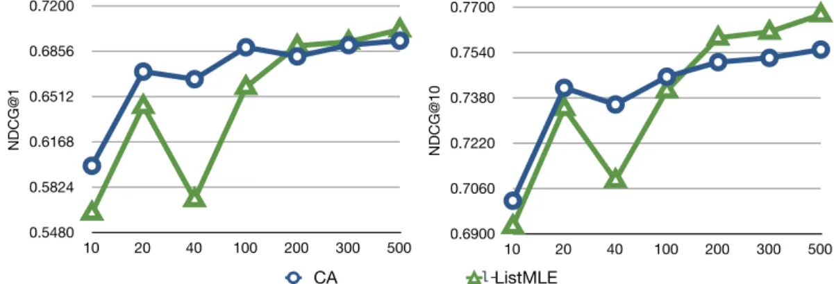
2.2 l-ListMLE and CA with different number of features. . . 34

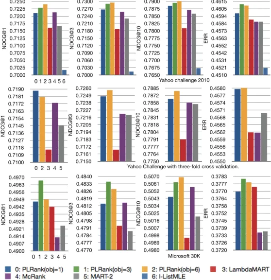
2.3 Comparison of several tree-based systems. . . 36

2.4 With different feature number, the comparison of the PLRank and the

LambdaMART systems on the synthetic dataset. The feature number in

the real distribution is 1000, and per query document number is 250. . . 40

3.1 Histogram of total improvements of OLE over SE. . . 60

3.2 Improvements (absolute %) of OLE over SE with McRank system when

the learning rate is set as 0.06.Each point in the figures has been averaged over a five-fold or three-fold cross-validation. . . 63

(10)

3.5 Improvements (absolute %) of OLE over SE with LambdaMart system when the learning rate is set as 0.06. Each point in the figures has been averaged over a five-fold or three-fold cross-validation. . . 66

3.6 Improvements (absolute %) of OLE over SE with LambdaMart system

when the learning rate is set as 0.1. Each point in the figures has been averaged over a five-fold or three-fold cross-validation. . . 67

3.7 Improvements (absolute %) of OLE over SE with LambdaMart system

when the learning rate is set as 0.12. Each point in the figures has been averaged over a five-fold or three-fold cross-validation. . . 68

3.8 Improvements (absolute %) of OLE over SE with RankBoost system when

3.9 Improvements (absolute %) of OLE over SE with RankBoost system when

the learning rate is set as 0.1.Each point in the figures has been averaged over a five-fold or three-fold cross-validation. . . 70 3.10 Improvements (absolute %) of OLE over SE with RankBoost system when

4.1 PL(k) with 500 L-BFGS iterations, k=1,3,5,7,9,12,15 compared with MIRA

(11)

List of Tables

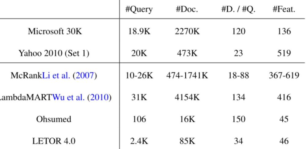
2.1 The top two datasets are used, while the others are as a reference. Ohsumed

is of LETOR 3.0. #D./#Q. means average document number per query. . 30

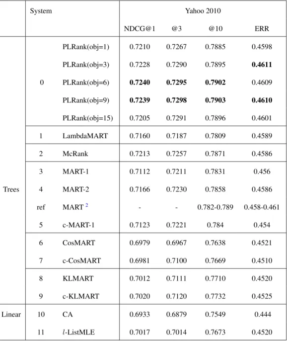
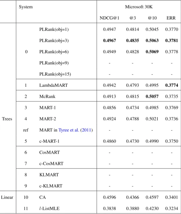
2.2 Main results on the Yahoo Challenge dataset. Results on the standard five splits of Microsoft data are averaged, and we follow the standard one split for the Yahoo data to compare to published results. System 1 is trained towards optimizing NDCG. System 10, CA, is a Coordinate Ascent based method directly maximizing NDCG. We provide results marked as “ref” reported in other papers. LambdaMART-Aug70 is trained on resampled training data, where our experiments are conducted on full training data. As PLRank(obj=6) in Microsoft data starts to decrease, we did not test more objectives. CosMART got an abnormally low score in Microsoft data asl-ListMLE, thus it is less meaningful to list them. . . 31 2.3 Main results on the Microsoft dataset. Results on the standard five splits

of Microsoft data are averaged, and we follow the standard one split for the Yahoo data to compare to published results. System 1 is trained to-wards optimizing NDCG. System 10, CA, is a Coordinate Ascent based method directly maximizing NDCG. We provide results marked as “ref” reported in other papers. LambdaMART-Aug70 is trained on resampled training data, where our experiments are conducted on full training data. As PLRank(obj=6) in Microsoft data starts to decrease, we did not test more objectives. CosMART got an abnormally low score in Microsoft data asl-ListMLE, thus it is less meaningful to list them. . . 32 2.4 Compression ratio of denominator terms in Eqn. (2.3) in considering

mul-tiple ground-truth permutations. . . 35 2.5 An industry level comparison in the standard Yahoo Challenge set 1 data

(12)

2.6 Sorted running time in the Microsoft dataset in a single computing core.

MT: MART. PRn: PLRank(obj=n). MR: McRank. . . 42

3.1 The top two datasets are used in this work and others are just a reference.

λ-MART is LambdaMART. Ohsumed is of letor 3.0. #D./#Q. means

av-erage document number per query. . . 55

3.2 Performances (%) of SE / OLE in the Yahoo Data with McRank model.

All results reported are averaged over self-defined three-fold. All results with over 0.1 point improvement are marked. . . 56

3.3 Performances (%) of SE / OLE in the Yahoo Data with LambdaMART

model. All results reported are averaged over self-defined three-fold. All results with over 0.1 point improvement are marked. . . 57

3.4 Performances (%) of SE / OLE in the Yahoo Data with RankBoost model.

All results reported are averaged over self-defined three-fold. All results with over 0.1 point improvement are marked. . . 58 4.1 The probability of the rankπ = (2,3,1)isp(r2)·p(r3)/(1−p(r2))in a

simplified form, as p(r2)

Z1 =p(r2)and p(r1)

Z3 = 1. . . 73 4.2 PL(k): Plackett-Luce model optimizing the ground-truth permutation with

length k. The significant symbols (+ at 0.05 level) are compared with MERT. The bold font numbers signifies better results compared to M(1) system. . . 77

(13)

Acknowledgment

First, I would like to give my appreciation to my Advisor, Prof. Shaojun Wang, who is like an amiable father but also strict on our work, and keeps giving endless encouragment and support, in the past several years.

Second, I would like to give my gratitude to Prof. Keke Chen, Prof. Michael Raymer, and Prof. Xinhui Zhang, for their invaluable time and advice as well as serving as my committees.

Third, I would like to give my thanks to my colleaguges, Shaodan Zhai, Ming Tan, Zhongliang Li, Raymond Kulhanek, Lu Chen, Wenbo Wang and other awesome guys, who accompanied me to go through the happiest days and the hardest days.

Finally, I would like to give my especial thanks to my family, and wife, for their supporting my work, understanding my decision in the work and life.

(14)

(15)

Introduction

1.1

Learning to Rank

1.1.1

Methodologies

The learning to rank task arises from practical real-world applications such as Google, Yahoo, Bing and other search engines, and has been flourishing for a decade. To put it simply, after a user inputs a query, the ranking system is designed to return a set of documents and rank them by their relevance to the input. Commonly used measures to quantify a rank quality of retrieved documents include MAP, ERR, NDCG, and etc.

The learning to rank task arises from real-world applications such as Google, Yahoo, and other search engines. A ranking system returns a set of documents and ranks them by their relevance to the query from a user.

Learning to rank techniques are influencing traditional natural language processing applications, such as model parameter trainingHopkins and May(2011b), and non-linear feature extractionSokolov et al.(2012);Toutanova and Ahn(2013).

(16)

basic ranking objects. This definition would not be affected by how to utilize features, e.g., linear and non-linear features.

The first methodology, point-wise based, breaks relationship between documents related to different queriesCossock and Zhang(2006);Crammer et al. (2001); Friedman (2001);Li et al.(2007), then uses traditional machine learning regression and classification techniques for training. For example, MART Friedman (2001) uses the regression tree technique to fit model outputs to their relevance scores; McRankLi et al.(2007) converts the rank procedure as a multi-class classification.

The second methodology, pair-wise based, considers the relationship among docu-ments related to the same queryCohen et al. (1999); Freund et al. (2003); Hazan et al. (2010);Herbrich et al.(1999);Joachims(2002);Quoc and Le(2007);Rudin(2009);Tsai et al.(2007);Wu et al. (2010), then adopts mature classification techniques to minimize the inversion number of documents by considering document pairs. For example, Rank-BoostFreund et al.(2003) plugs the exponential loss of document pairs into a framework of Adaboost; RankSVMHerbrich et al.(1999);Joachims(2002) uses SVM to perform a binary classification on the document pairs; LambdaRankQuoc and Le(2007) and Lamb-daMARTWu et al. (2010) take into account the influence of a correctly classified docu-ment pair to the objective measures, and achieve a big success.

The third methodology,list-wise based, treats a permutation of a set of documents as a basic unit, and builds loss functions on them Cao et al. (2007); Metzler and Croft (2007); Ravikumar et al.(2011); Tan et al. (2013a); Xia et al. (2009, 2008); Xu and Li (2007); Xu et al. (2008). Because exact losses of performance measures are step-wise, non-differentiable as well as non-convex with respect to model parameters, most work

(17)

in this methodology resort to suitable surrogate functions. These surrogate functions are either not directly related to ranking performance measures Cao et al.(2007); Qin et al. (2008);Xia et al.(2009,2008), or just continuous and differentiable approximation bounds of ranking measures Chakrabarti et al. (2008); Chapelle and Wu (2010); Le and Smola (2007);Qin et al.(2010a);Taylor et al.(2008);Valizadegan et al.(2009);Wu et al.(2010); Xu et al. (2008); Xu and Li (2007); Yue et al. (2007). To further decrease the gap be-tween optimization objectives and performance measures, some work attempt to directly optimize objective measures and show promising results. For example, in Metzler and Croft(2007);Tan et al.(2013a), the authors use a coordinate ascent framework to directly optimize performance measures, and DirectRank in Tan et al.(2013a) is much faster in practice. However, both their work still can not match the state-of-the-art systems in large data sets when decision trees are used1.

1.1.2

Basic Notations

Given a set of queriesQ = {q1, . . . , q|Q|}, each queryqi is associated with a set of

can-didate relevant documentsDi ={di1, . . . , di|Di|}and a corresponding vector of relevance scoresri = {r1i, . . . , ri|Di|} for each Di. The relevance score is usually an integer, and greater value means more related for the document to the query. An M-dimensional

feature vectorh(d) = [h1(d|q), . . . , hM(d|q)]T is created for each query-document pair,

whereht(·)s are predefined real-value feature functions.

A ranking functionf is designed to score each query-document pair, and the

doc-1_{Tan et al.}_{Tan et al.}₍_2013a_{) use a mixed strategy, which borrows boosted trees generated from MART,} to compete with LambdaMART. Their strategy should be treated as a system combination technique rather than a single ranking model.

(18)

uments associated with the same query are ranked by their scores and returned to users. Since these documents have a fixed ground truth rank with its corresponding query, our goal is to find an optimal ranking function which returns such a rank of related documents that is as close to the ground truth rank as possible. Industry-level applications often adopt regression trees to construct the ranking function, and use Newton Formula to calculate the output values of leaves of trees.

Generally, ranking functions use only linear information of original featuresh(d|q) or their nonlinear information. The linear form is asf(d|q) = wT _·_h₍_d₎_{, where}_w ₌

[w1, . . . , wM]T ∈ RM is the model parameter. The nonlinear form often adopts regression

trees, kernel technique, and neural network.

Several measures have been used to quantify the quality of a rank, such as NDCG@K,

ERR, MAP etc. In this paper, we use the most popular NDCG@Kand ERRChapelle and

Chang(2011) as the performance measures.

1.1.3

Metrics

Normalized Discounted Cumulative Gain (NDCG) (Järvelin and Kekäläinen(2002)) is a popular metric for relevance judgments. It assigns exponentially high weight to highly relevant documents.

Given a training query qi and the ranking function f, the relevant documentsDi is

(19)

NDCG(qi, f) = DCG(qi, f) Idea DCG (1.1) DCG = K X j=1 2rij−₁ log(1 +j) (1.2)

Usually, NDCG is trimmed at a certain ranking levelK, such as, 1, 3, 10.

ERR is a novel metric based on the cascade user model (Chapelle et al.(2009)). It is defined as the expected reciprocal rank at which the user will stop his search under this model. The resulting formula is:

ERR = n X j=1 1 jP(user stops atj) = n X j=1 1 jR(j) j−1 Y t=1 (1−R(t) (1.3) R(t) = 2 yti−1 16 (1.4)

1.1.4

Gradient Boosting, Square Error (SE) and Regression Tree

We review gradient boostingFriedman(2001) as a general framework for function approx-imation using regression trees as the weak learners, which has been the most successful approach for learning to rank models.

Gradient boosting iteratively finds an additive predictorf(·) ∈ H that minimizes a loss function L. At thetth iteration, a new weak learnergt(·) is selected to be added to

(20)

current predictorft(·)to construct a new predictor,

ft+1(·) =ft(·) +αgt(·) (1.5)

whereαis the learning rate.

r(·) = −L0(ft(·)) (1.6)

In gradient boosting, according to the following squared loss,gt(·)is chosen as the

one most parallel to the pseudo-response− ∂L

∂ft(·), which is negative derivative of the loss function in functional space.

gt(·) = arg min g∈H k − ∂L ∂ft(·) −g(·)k2 2 (1.7)

To fit a regression tree, the data in each internal tree node is greedily split into two parts by minimizing Eqn. (1.7), and this procedure recursively iterates until a predefined condition is satisfied. This tree construction procedure is applicable for any differentiable loss function. The complexity of a regression tree is usually controlled by the tree height or leaf number. In learning to rank, the latter is more flexible, thus is adopted in this work by default.

In one node, we enumerate all features as well as their possible thresholds, and find the best feature-threshold pair with the smallest error to conduct binary splitting on the current node.

(21)

two parts. The samples, whose feature values are less thanv, are denoted asDl, and others

are denoted asDr. Then the squared error is defined as

SE(v) = X

d∈Dl

(r(d)−r1)2+ X

d∈Dr

(r(d)−r2)2 (1.8)

wherer1,r2are average pseudo-response of samples on the left and right respectively.

1.1.5

Classification and Learning to Rank

Cossock et al.Cossock and Zhang(2006);Li et al.(2007) proved that the negative unnor-malized NDCG value is upper-bounded by multi-class classification error, where NDCG is an important measure in learning to rank. Thus Li et al.Li et al.(2007) proposed a multi-class multi-classification based ranking systems called McRank in gradient boosting framework. McRank utilizes classic logistic regression, which models class probabilitypk(d)as

pk(d) =p(y(d) =k|d) =

expfk₍_d₎

PK

c=0expfc(d)

(1.9)

wherefc₍_·₎_{is an additive predictor function for the}_c_{th class.}

The objective loss function is the negative log-likelihood, defined as

L=−X d K X c=0 I(y(d) =c) logpc(d) (1.10)

(22)

Weighted Square Error (WSE) in Logitboost

In classification, this loss function (Eqn. 1.10) resulted in the well-known system Logit-Boost, which first used WSE to fit a regression tree. WSE utilizes both first- and second-order derivative information.

WSE uses a different definition of the response valuer(·)from that in SE (Eqn.1.6), and defines an extra weightw(·)for each sample.

r(·) = −L0₍_f

t(·))/L00(ft(·))

w(·) = L00₍_f

t(·))

(1.11)

The splitting principle is minimizing the following weighted error

W SE(v) = P_d_∈_D lw(d)(r(d)−r1) 2₊P d∈Drw(d)(r(d)−r2) 2 − P d∈Dw(d)(r(d)−¯r)2 (1.12) where r1 = P d∈Dlwi·r(d) P d∈Dlwi r2 = P d∈Drwi·r(d) P d∈Drwi r = P d∈Dwi·r(d) P d∈Dwi (1.13)

Regarding LogitBoost, the response and weight values, by Eqn. 1.11, are set as w(d) =pk(d)(1−pk(d)),r(d) = I

(y(d)=k)−pk(d)

(23)

The responser(d)might become huge and lead to unsteadiness whenpk(d)is approaching

0or1. Though Friedman et al.Friedman et al.(2000) described some heuristics to smooth the response values, LogitBoost was still believed numerically unstableFriedman(2001); Li(2010b);Friedman et al.(2000). As a result, McRank is actually using SE and gradient boosting to fit regression trees (Section1.1.4), rather than LogitBoost.

Robust Weighted Square Error (RWSE) in Logitboost

LiLi(2010b) rederived Eqn. 1.12and proposed a stable version of WSE for LogitBoost, which is shown below

RW SE(v) = [ P d∈Dw(d)r(d)] 2 P d∈Dw(d) − " [P d∈Dlw(d)r(d)] 2 P d∈Dlw(d) +[ P d∈Drw(d)r(d)] 2 P d∈Drw(d) # (1.14)

Since the denominators in Eqn. 1.14are summation of a set of weightsw(·), which are less likely to be close to zero in practical applications, and RWSE is hence more stable than WSE.

After fitting a regression tree by either SE or (R)WSE, the data aggregated in the same leaf is assigned with a value by weighted averaging responses (Eqn.1.13).

Li mentioned, Eqn. 1.13 could be interpreted as a weighted average in (R)WSE; while in gradient boosting, it is interpreted as a one-step Newton update. It looks like a coincidence. In next section, we propose a unified splitting principle, which not only

(24)

clearly explains the relationship of these principles, but also could be extended to more complex loss functions. Also, our method generates Li’s robust version directly.

1.2

Our Work

1.2.1

Plackett-Luce Model for Learning-to-Rank Task

Our work utilizes an elegant list-wise surrogate function called Plackett-Luce (PL) loss, which was first proposed in 1975 Plackett (1975) for horse gambling. Cao et al. Cao et al.(2007) introduce it to the learning to rank task by using it to model the probabilistic distribution of a set of documents given a query, where the training is conducted by min-imizing the KL distance between the probability distribution for the ranking model and that for the ground truth. Later Xia et al.Xia et al.(2009, 2008) provide a model called ListMLE, which instead maximizes the likelihood of ground-truth permutations defined in the PL loss. ListMLE could be viewed as a general framework to utilize linear and non-linear features, however, as its non-linear system has not been developed, we refer tol-ListMLE as its linear version hereafter. Because public large-scale datasets were not

available until 2010, many properties of the PL loss are not revealed inl-ListMLE. Even

though l-ListMLE performs pretty well on some datasets, it is rather unstable in many

other cases, especially when compared with direct optimization based models, e.g. Direc-tRankTan et al.(2013a) and LambdaRankQuoc and Le(2007). Although not necessarily the best, DirectRank and LambdaRank often show reasonable good performance, whilel

(25)

For example, on the Microsoft 30K data, the largest publicly available real world dataset, l-ListMLE is approximately 7.6 points worse than the coordinate ascent based method

Metzler and Croft(2007) in terms of NDCG scores. Although, Xia et al. Xia et al.(2009) further proved the PL loss is consistent with NDCG@K under certain assumptions, it is not guaranteed to achieve a reasonable performance on practical applications that use data sets with limited size, and the unstable performance behavior greatly limits wide spread real-world applications for the ListMLE model.

Understanding why the PL loss fails in some datasets is important to design more effective algorithms, thus we conduct experiments to analyze these datasets, and figure out one principle as the condition for the PL loss, which states that as compared to average document number per query, the number of features should be large enough. Therefore in order to gain better performance, we have to use more features for PL loss. There are several ways to enrich features of datasets:kernel mapping,neural network mapping, and

gradient boosting. We select the gradient boosting with decision trees as weak rankers in this work due to the convenient comparison with LambdaMART, and leave the others for further work. A merit of the PL loss is its concise formula to compute functional gradients, Eqn. (2.11), which results in our ranking system, called PLRank.

As suggested in Chapelle and Chang (2011), real-world datasets are closer to the scenario of search engine applications and have much smaller fluctuations in terms of performance. We conduct experiments on two publicly released real-world datasets. As far as we know, these datasets are larger than any used in previous research papers, except Wu et al.(2010)2_{. To compare with other list-wise based methods, we also extend three}

(26)

extra consistent list-wise surrogate functions in Ravikumar et al. (2011) in the gradient boosting framework. We find that PLRank not only maintains the merits of the PL loss, but also greatly alleviates the instability problem ofl-ListMLE. PLRank has the same time

complexity with LambdaMART, and isM times as fast as McRank3.

1.2.2

Analysis of Regression Tree Fitting Algorithms in Learning to

Rank

Top practical learning to ranking systems are adopting gradient boosting framework and using regression trees as weak learners. These systems performed much better than lin-ear systems on real-world datasets such as in Yahoo challenge 2010Chapelle and Chang (2011), and another real-world dataset Microsoft 30KTan et al. (2013a). Among these systems, LambdaMARTWu et al.(2010);Burges et al.(2011), a pair-wise based model, gained an excellent reputation in Yahoo challenge; MARTFriedman(2001), a point-wise based, is a regression model which utilizes least square loss as objective loss function, and McRankLi et al.(2007)4, a point-wise based, uses multi-class classification technique and converts predictions into ranking. For industry applications, gradient boosting combined with regression trees appears to be a standard practice.

An important finding was made by Cossock et al. Li et al. (2007); Cossock and Zhang(2006) that has created a bridge between learning to rank and classification.They proved that an important measure NDCG in learning to rank is bounded by multi-class classification error. This leads to McRank system. This insight opens a door for learning

3_M_{is the number of different relevance scores in measuring a document.} 4_{Li et al. call the model of McRank as MART in the scenario of classification.}

(27)

SE

Gradient Boosting MART

SE

LogitBoost LambdaMART McRank

(R)WSE

OLE

Saturday, August 1, 15

Figure 1.1: Three node splitting principles in decision tree construction, namely Square Error (SE) in Gradient Boosting framework, Robust Weighted Square Error (RWSE) in the LogitBoost system, and Objective Loss Based Error (OLE) in this paper, as well as their relations. All real-line arrows denote known relations, and dotted-line arrows denote our contribution.

to rank, as we could borrow state-of-the-art techniques from those developed for multi-class multi-classification.

In multi-class classification area, there is a work that fits a regression tree using weighted least square error (WSE) principle. It uses both first- and second-order informa-tion, not only first-order like SE in gradient boosting. LogitBoostFriedman et al.(2000) and its robust versions Li (2010a,b) are examples of such applications. A comparison between gradient boosting using SE, and LogitBoost using WSE for classification task Friedman(2001) shows that the latter is slightly better. As WSE is empirically considered as unstable in practiceFriedman et al.(2000);Li (2010b); Friedman(2001), Li et al. Li (2010b) obtained a stable form of WSE, called RWSE.

However, both WSE and RWSE are somewhat hard to understand and have no clear theoretical explanation. Li et al. thus proposed an interesting question in Section 2.3 ofLi (2010b):in determining the output of a leaf of a regression tree, the one-step Newton for-mula from gradient boosting coincides with the weighted averaging from WSE.Moreover,

(28)

RWSE looks pretty concise, which might be considered to be applicable for any ranking models in addition to LogitBoost and its variants. These issues drive us to consider from another point of view.

We propose a general regression tree fitting principle for ranking models, called least objective loss based error (OLE). It only requires simple computation to derive exact for-mula and is easy-to-understand. Under this principle, besides clearly answering the afore-mentioned question, we analyze a variety of ranking systems to build a relationship be-tween SE, (R)WSE and OLE, which is shown in Figure1.1. Experiments in real-world datasets show OLE improves most of results over SE.

1.2.3

A Simple Discriminative Training Method for Machine

Trans-lation with Large-Scale Features

Since OchOch(2003) proposed minimum error rate training (MERT) to exactly optimize objective evaluation measures, MERT has become a standard model tuning technique in statistical machine translation (SMT). Though MERT performs better by improving its searching algorithmMacherey et al. (2008);Cer et al. (2008); Galley and Quirk (2011); Moore and Quirk(2008), it does not work reasonably when there are lots of features5_{. As}

a result, margin infused relaxed algorithms (MIRA) dominate in this caseMcDonald et al. (2005);Watanabe et al.(2007);Chiang et al.(2008);Tan et al.(2013b);Cherry and Foster (2012).

In SMT, MIRAs consider margin losses related to sentence-level BLEUs. However,

5_{The regularized MERT seems promising from Galley et al.} _{Galley et al.}₍₂₀₁₃_{) at the cost of model} complexity.

(29)

since the BLEU is not decomposable into each sentence, these MIRA algorithms use some heuristics to compute the exact losses, e.g., pseudo-document Chiang et al. (2008), and document-level lossTan et al.(2013b).

Recently, another successful work in large-scale feature tuning include force decod-ing basedYu et al.(2013), classification basedHopkins and May(2011a).

We aim to provide a simpler tuning method for large-scale features than MIRAs. Out motivation derives from an observation on MERT. As MERT considers the quality of only top1hypothesis set, there might have more-than-one set of parameters, which have similar top1 performances in tuning, but have very different topN hypotheses. Empirically, we expect an ideal model to benefit the total N-best list. That is, better hypotheses should be assigned with higher ranks, and this might decrease the error risk of top1 result on unseen data.

PlackettPlackett(1975) offered an easy-to-understand theory of modeling a permu-tation. An N-best list is generated by sampling without replacement. Theith hypothesis

to sample relies on those ranked after it, instead of on the whole list. This model also supports a partial permutation which accounts for topk positions in a list, regardless of

the remaining. When takingk as 1, this model reduces to a standard conditional

proba-bilistic training, whose dual problem is actual the maximum entropy basedOch and Ney (2002). Although OchOch (2003) substituted direct error optimization for a maximum entropy based training, probabilistic models correlate with BLEU well when features are rich enough. The similar claim also appears inZhu and Hastie(2001). This also make the new method be applicable in large-scale features.

(30)

Plackett-Luce Model for

Learning-to-Rank Task

2.1

Plackett-Luce Loss for Learning to Rank

The Plackett-Luce model was first proposed by Plackett Plackett (1975) to predict the ranks of horses in gambling. Consider a horse racing game with five horses. Suppose a probability distributionP on their abilities to win a race, then a rank of these horses can be understood as a generative procedure. Suppose we want to know the probability of a top3 rank2,3,5. The result can be computed as follows:

Being the champion for the 2nd horse, the probability isp2 among five candidates.

Being the runner-up for the 3rd horse, the probabilityp3 has to be normalized among the

remaining four horses, which leads top3/(p1+p3+p4+p5). Being the third winner for

the 5th horse, its probability among the remaining three horses becomesp5/(p1+p4+p5).

So the probability of the rank2,3,5is their product. It is not difficult to see that the most

(31)

The key idea for the Plackett-Luce model is the choice in theith position in a rankπ

only depends on the candidates not chosen at previous positions.

2.1.1

Plackett-Luce Loss with Linear Features

In learning to rank, each training sample has been labeled with a relevance score, so the ground-truth permutation of documents related to theith query can be easily obtained and

denoted asπi, where πi(j)denotes the index of the document in the jth position of the

ground-truth permutation. We note that πi is not obligatory to be a full rank, as we may

only care about the topKdocuments.

Consider a ranking function with linear features, the probability of a set of candidate relevant documentsDiassociated with a queryqi is defined as

p(di_e) = exp{h(d i e)T ·w} P d∈Diexp{h(d) T _·_w_} (2.1)

The probability of the Plackett-Luce model to generate a rankπiis given as

p(πi,w) = |πi| Y j=1 p(di_π_i(_j₎|Ci,j) (2.2) p(di_e|Ci,j) = p(di_e) P d∈Ci,jp(d) (2.3)

whereCi,j =Di− {d_πi_i(1), . . . di_π_i(_j−1)}.

The training objective is to maximize the log-likelihood of all expected ranks over all queries and retrieved documents with corresponding ranks in the training data with a

(32)

zero-mean and unit-variance Gaussian prior parameterized byw. L= log{Y i p(πi,w)} − 1 2w T_w _(2.4)

The gradient can be calculated as follows,

∂L ∂w = X i X j {h(di_π_i(_j₎)− X d∈Ci,j (h(d)·p(d|Ci,j))} −w

Since the log-likelihood function is smooth, differentiable, and concave with the weight vectorw, global optimum guarantee is satisfied.

2.1.2

Plackett-Luce Loss with Regression Trees

In this paper, we build ensemble regression trees for the Plackett-Luce loss in the gradient boosting framework, Alg. 1 summarizes the main procedure. We first describe how to compute the pseudo response and output value for fitting a regression tree, and then we provide more analysis for this new model.

At thetth iteration, all fitted regression trees constitute the current predictorft(·), and

the Eqn. (2.1) can be rewritten as

p(di_e) = exp{ft(d i e)} P|Di| k=1exp{ft(d i k)} (2.5)

We limit|π| = K, and adopt Eqn. (2.4) without a normalization as our objective1_. 1_{The model complexity of regression trees is often controlled by the learning rate}_{α, different from the}

(33)

Plugging Eqn. (2.5) into Eqn. (2.4), and taking derivative with respect toft(·), we obtain

L0(ft(d)) =I(d∈topKground-truth)−

X

C s.t. d∈C

p(d|C) (2.6)

where I(·)denotes the indicator function. When I(·)returns 0 for the current document, the size of{C}equalsK, otherwise it is smaller.

We follow Eqn. (1.7) to fit a regression tree gt(·). Denotes the documents falling

in the leaf U as Ud. We set the output of the leaf U as gt(d ∈ Ud) = −v, and v is

optimized independently from other leaves. Following Eqn. (1.5), we constructft+1(·)for documents inUd.

We adjust v to maximize the log-likelihoodL. Thus L has been reinterpreted as a function ofv. We rewrite Eqn. (2.5) as

p(di_e) = exp{ft(d i e)−I(die ∈Ud)·αv} P|Di| k=1exp{ft(dik)−I(die ∈Ud)·αv)} (2.7)

By the Newton method, we have

v = L 0₍_v _{= 0)} L00₍_v _{= 0)} (2.8) L0(v = 0) = X d∈Ud L0(ft(d)) (2.9) L00(v = 0) = X C p0·(p0−1) (2.10) p0 = X d∈Ud∩C p(d|C) (2.11)

(34)

Algorithm 1PLRank

Require: DocumentsD ={D1,D2, . . .};K defines topK documents of a ground-truth rank;T defines regression tree number;Ldefines leaf number;αdefines learning rate.

1: f1(·)←BackGroundModel(·) .Initialization for model adaptation. None by default.

2: forDiinDdo

3: Randomly shuffleDi

4: SortDiby relevances. .We could build several ground-truth permutations. 5: end for

6: fort= 1toT do

7: Resp(d∈S

Di)← −L0(ft(d)) .Compute pseudo response following Equ.2.6.

8: Fit aL-leaf treegtonResp. .By Eqn. (1.7) by default.

9: forleafU ingtdo

10: v ← L0₍_v _{= 0)}_/_L00₍_v _{= 0)} _._{Set output of current leaf by Eqn. (}_2.11₎

11: gt(d∈Ud)← −v

12: end for

ft+1 ←ft+αgt .Eqn. (1.5)

13: end for

returnfT+1

To clarify this procedure, we take one query with four related documents as an ex-ample. Suppose the four documents d1, d2, d3, d4 are sorted in a descending order with

their relevance scores. In an other word, the ground-truth permutation isd1, d2, d3, d4. Let

their scores after some iterations, from current predictorft(·), bes1, s2, s3, s4respectively for abbreviation. Considering the top 2documents of the ground-truth permutation, the log-likelihood is

L = s1 −log{exps1+ exps2+ exps3+ exps4} + s2 −log{exps2+ exps3+ exps4}

(35)

In this toy example, the sampless3, s4 haveK = 2contextual probabilities.

Supposes1,s3 fall into the same leaf of a regression tree, then

L0₍_v _{= 0)} _{= 1}₋_p₍_s 1|C1) + 0− {p(s3|C1) +p(s3|C2)} L00₍_v _{= 0) = (}_p₍_s 1|C1) +p(s3|C1))·(p(s1|C1) + p(s3|C1)−1) +p(s3|C2)·(p(s3|C2)−1) whereC1 ={s1, s2, s3, s4},C2 ={s2, s3, s4}.

In the following, we describe more details of Alg. 1 that relate to initialization of models (line 1), selection of ground-truth permutation (line 3-4).

Initialization of Models

As a statistical model is sensitive to data genres, a trivial yet effective way is to use more data for training. In some applications, data in the objective genre may be sparse, while general genre data is plenty, then it is useful to explore model adaptation. Borrowing the idea from adaptive LambdaMART Wu et al. (2010), our model could also first train a background model on plenty of general genre data. Then we assign the resulting model to

(36)

initialize our Alg1(line 1), and continue to train our model using on objective genre data. In this paper, we are not focusing on the adaptation experiments, and we initialize to zero.

Selection of Ground-Truth Permutations

In learning to rank, as the relevance scores are scattered among limited integers, e.g., 0 to 10 inclusively, there are many ties in the scores, this would impact the determination of ideal permutations and our training objective. We analyze and compare three strategies on toy documentsd1, d2, d3, d4with relevance scores4,0,4,4, and consider top4

ground-truth documents.

The first one is a stable sort compatible with input. If two documents are equal in relevance scores, their relative rank in the ground-truth permutation should comply with the original input. Hence, the ground truth permutation in the first strategy should be d1, d3, d4, d2.

The second one is random selection. This strategy has been straightforwardly im-plemented in Alg. 1 by firstly randomly shuffling input data and then invoking the first strategy. This strategy is also the default setting in Xia et al.Xia et al.(2009,2008).

The third one considers multiple ground-truth permutations (looping lines 2-5 in Alg. 1). As the number of all permutation possibilities is huge, we randomly select several ground-truth ranks and store them compactly in terms of data structure. For instance, the ground truth permutation d1, d3, d4, d2 consists of three contextual terms,

C1 = {d1, d2, d3, d4}, C2 = {d2, d3, d4}, C3 = {d2, d4}, while adding a second permu-tationd1, d4, d3, d2 leads to merely one extra termC4 = {d2, d3}, rather than new three terms. The statistics about this issue on Yahoo 2010 and Microsoft 30k datasets are

(37)

re-ported in Table2.4. We use PLRank(obj=num) to denote different number of objectives.

Greedy Construction of Regression Tree

Since all tree fitting algorithms are conducted node by node, we only need to focus on the smallest sub-problem: given some features f and pseudo-response Resp(d) of each

document d, how do we select the best threshold to optimize the objective? Suppose

documents are sorted in an ascending order, denoted asd1, . . . , dN, then there are N −1

positions to define the threshold. Eqn. (1.7) defines such an optimal choice under least square loss. I∗ = arg min I X i≤I (Resp(di)−r¯1)2+ X I<j (Resp(dj)−r¯2)2 (2.12)

wherer¯1is the average pseudo-response of documents in the left part, andr¯2is the average

in the right part. If the resulting two nodes are leaf nodes, thenr¯1,r¯2 are set as the output

of leafs respectively.

Currently almost all tree based systems in learning to rank follow Eqn. (1.7) to fit a regression tree, which only uses the first order gradient of the least square loss rather than directly minimizing surrogate loss. In next section, we would introduce an effective construction algorithm which utilizes the second-order gradient information, and many systems such as McRank and our proposed PRRank could be further improved.

Theorem8suggests that the classic tree fitting algorithm in gradient boosting is very suitable for the least-square loss function, on which MART system is based, and this could explain why MART system actually performs extremely well in our experiments.

(38)

By default, in our experiments, all systems use the classic tree fitting algorithm to explore the differences resulting from loss functions only.

Stable Gradients

In the implementations of ranking systems, we often face the following numerical com-putation problem that leads to unstable performance: when the second derivative is small, the Newton iteration returns an abnormally huge quantity. Li et al. Li(2010b) explored a method to somewhat overcome this problem. Here we adopt another simple yet efficient tactic, exerting a small variation (line 12).

As the optimization objective is concave with respect to the output v of a leaf, the

second derivative is guaranteed to be negative by optimization theoryBazaraa et al.(2006). If we set β to be a positive number, it forces Gto have an at least β margin from zero.

Thus we simply setβ as 1 which works well in practice.

We find that there is another explanation for thisβ, which can be viewed as an effect

ofl2 norm ofαin Eqn. (2.4). The first derivative of Eqn. (2.4) inα = 0equalsL0(v = 0) in Eqn. (2.11); its second derivative equals L00₍_v _{= 0)}_{in Eqn. (}_??_{) minus}_α_{. This tactic} doesn’t influence system performance asL00₍_v _{= 0)}_{is constantly much greater than}_β _in large dataset.

2.1.3

Training with Plackett-Luce Loss

Regarding linear features, Xia et al. Xia et al. (2009, 2008) adopt a neural network to maximize the log-likelihood of expected ranks. The neural network works well in small

(39)

datasets, e.g. LETOR, while it also requires suitable settings on hidden layer structure and the number of hidden neurons.

As our experiments are conducted on real-world datasets, we instead use L-BFGS Byrd et al.(1995) for parameter tuning to gain faster convergence speed. It is observed that overfitting often occurs in small data sets, while in large datasets the log-likelihood correlates with ranking measures very well.

Regarding non-linear features, kernel technique could map them into a linear form in a high dimensional space, and then the neural network based training in Xia et al.’s work or LBFGS are applicable, provided that the new dimension is acceptable in practice. However, in the case of regression trees, it is impractical to expand all dimensions, which is why we propose our new algorithm. We are following the boosting framework, which iteratively fits high-quality decision trees, to maximize the objective log-likelihood.

2.1.4

Transformation between PL and McRank

McRank is a multi-class classification based ranking system first proposed by Li et al. Li et al.(2007). They proved that the unnormalized NDCG is bounded by classification er-rors, it is also well known that the log-loss is an upper bound of classification error, thus maximizing the log-likelihood is nothing but minimizing an upper bound of the unnormal-ized NDCG. As shown inLi et al.(2007), the ordinal classification version performs quite closely to its classification version; we use the latter hereafter.

We discover an interesting relationship between the PL model and the McRank model after a suitable transformation of datasets. Being a point-wise based method, McRank deals with data in a form of(H, r), where H is a feature vector of a document, andr is

(40)

its relevance score which is used as its category. Suppose the maximum relevance in the dataset isT, then in the view of McRank, the ranking problem is actually a(T + 1)-class

classification.

We now further transform this problem as the following: Each original document (H, r)extends the feature dimension by T times, filling with zero, and rewrites its new

relevance as 1. ([ |H|·r z }| { 0, . . .0, H, |H|·(T−r) z }| { 0, . . .0 ],1)

Insert extraT pseudo-documents for each original document with the feature dimension

as(T + 1)· |H|, and rewrite their new relevances as 0. The pseudo-documents are then defined as ([ |H|·r0 z }| { 0, . . .0, H, |H|·(T−r0₎ z }| { 0, . . .0 ],0) wherer0 ∈[0, T], andr0 6=r.

In the resulting dataset, a new pseudo-query is created to relate toT + 1documents,

and actually exclusively relates to one document of the original data. Among theseT + 1

documents, only one is redefined as relevant, with others as irrelevant to the pseudo-query. We invoke our PL ranker, setting top 1 document of a ground truth permutation as the optimization objective to solve the McRank model equivalently.

The discussion above only provides a theoretical analysis of these two ranking mod-els, and in practice we do not adopt this transformation since it expands the dataset by (T+ 1)2_{times in term of feature dimension and document number. Moreover the McRank}

model specifies an additional sum-to-one restriction, even though the two methods indeed utilize the same optimization objective.

(41)

In other areas such as natural language processing, many problems can be formulated as a ranking problem, while the definition of relevance scores is often no longer a discrete integer as in learning to rank. In this case, the McRank model may be not applicable, and the PL model is more promising instead.

2.1.5

Comparison with Other Consistent List-wise Methods

Calauzenes et al. Calauz`enes et al.(2012) have proved that no consistent surrogate func-tion exists for ERR and MAP. However, regarding NDCG, Xia et al. Xia et al. (2009) proved that the ListMLE model is consistent with NDCG@K. They also modified two other losses, cosine and KL divergence, to make them NDCG@K consistent. As Xia et al. have compared them in their work, we thus compare the PL loss with three other consistent versions proposed inRavikumar et al.(2011),squared loss,cosine, andKL di-vergence, which were proved to be consistent with the whole list, in the case of boosted trees.

We pay special attention to the first one since it has three different implementations. Letsdenote a score vector of all documents,rdenote the corresponding relevance vector, andG(r) = 2r₋₁_{. The consistent and inconsistent equations in terms of square loss in} Ravikumar et al.(2011) are

φconsistent_sq (s,r) =ks− G(r) kG(r)kD k2 2 (2.13) and φinconsistent_sq (s,r) =ks−G(r)k2 2 (2.14)

(42)

where the normk · kD defines the DCG value of a ground-truth permutation per query.

A third equation inCossock and Zhang(2006) is also inconsistent with NDCG.

φinconsistent_sq (s,r) =ks−r k2₂ (2.15)

All boosting systems with the least-squares loss are called MART in this paper. The two inconsistent versions are point-wise based, and the consistent one is list-wise based since the norm k · kD is operated by query. We remove detailed discussion about the

functional gradients for all surrogates above due to space limitation.

2.2

Experiments

We studied the performance of the proposed algorithm in two real world datasets, Yahoo challenge 2010 and Microsoft 30K. We implemented 9 baseline ranking systems in C++, which use boosted trees as features. System 1 is LambdaMART. System 2 is McRank. System 3 is MART-1 which is the first inconsistent version of MART (Eqn. (2.14)). Sys-tem 4 is MART-2 which is the second inconsistent version of MART (Eqn.2.15). System 5 is c-MART-1 which is a consistent version of MART-1 (Eqn. (2.13)). System 6 is Cos-MART which is an inconsistent version of cosine distance loss with boosted trees. System 7 is c-CosMART which is a consistent version of CosMART. System 8 is KLMART which is a MART using the KL distance. System 9 is c-KLMART which is a consistent version of KLMART.

(43)

systems. System 10 is based on a heuristic coordinate ascend (CA) based optimization Metzler and Croft(2007) which uses linear features and optimizes NDCG directly. CA is used as a reference system to represent the average performance of linear systems due to its relatively stable and good performances among a variety of linear models in different datasets, including the datasets used in this work, as shown in the experiments of Tan et al. Tan et al.(2013a). This system is akin to the one proposed by Tan et al., but the latter is an exact coordinate ascent optimization ranking method. We also used the experimental results in Tan et al.(2013a) as a reference here. System 11 is l-ListMLE that optimizes

top10retrieved documents.

We set up the same parameters as inWu et al. (2010) for all systems. The learning rateαis 0.1 (line 15 in Alg. 1). We set the number of decision tree leaves as 30, which is

a classic setting. As in real world datasets, McRank requires more iterations to converge, thus we use 2500 boosted trees as a final model, and use 1000 boosted trees for other systems. Regarding to PLRank, as we mainly concentrate on NDCG@10, we setK to 10

to optimize top10documents of ground-truth permutations. All results are reported with NDCG@(1,3,10) and ERR scores.

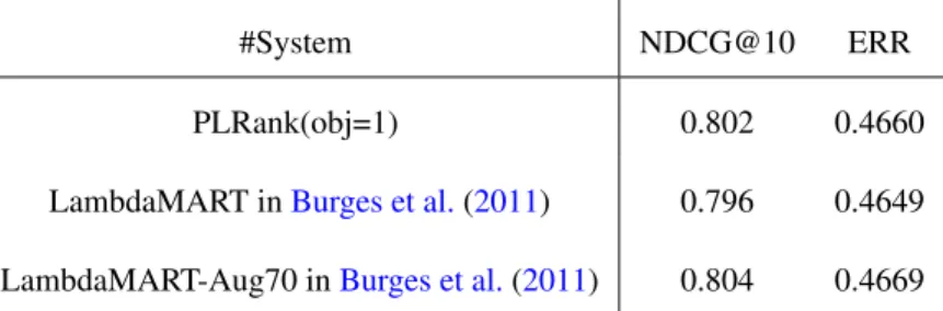
In order to examine the industry-level performance of our system, we search exhaus-tively parameters to compare to the Yahoo Challenge resultsChapelle and Chang(2011) in Table2.5.

2.2.1

Datasets

The LETOR benchmark datasets released in 2007 Qin et al. (2010b) have significantly boosted the development of learning to rank algorithms since researchers could compare

(44)

their algorithms on the same datasets for the first time. But unfortunately, the sizes of the datasets in LETOR are several orders of magnitude smaller than the ones used by search engine companies. Several researchers have noticed that the conclusions drawn from experiments based on LETOR datasets are unstable and quite different from the ones based on large real datasetsChapelle and Chang (2011). Thus in this work, we attempt to make stable system comparisons by using as large datasets as possible, and we use two real world datasets, Yahoo challenge 2010 and Microsoft 30K. The statistics oh these three data sets are reported in Table2.1which might a bit different from those inChapelle and Chang(2011) as we only give the statistics of training datasets.

#Query #Doc. #D. / #Q. #Feat.

Microsoft 30K 18.9K 2270K 120 136 Yahoo 2010 (Set 1) 20K 473K 23 519 McRankLi et al.(2007) 10-26K 474-1741K 18-88 367-619 LambdaMARTWu et al.(2010) 31K 4154K 134 416 Ohsumed 106 16K 150 45 LETOR 4.0 2.4K 85K 34 46

Table 2.1: The top two datasets are used, while the others are as a reference. Ohsumed is of LETOR 3.0. #D./#Q. means average document number per query.

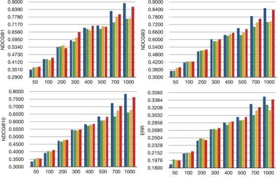
Microsoft 30K is the largest publicly released dataset in terms of the document num-ber. As its official release has provided a standard 5-fold split, we report average results. Regarding the Yahoo dataset, it only provides a 1-fold split. In order to compare to other released systems, we report results on the standard 1-fold split in Table 2.3, and report average results on a randomly generated 3-fold split in Figure2.3.

(45)

System Yahoo 2010 NDCG@1 @3 @10 ERR PLRank(obj=1) 0.7210 0.7267 0.7885 0.4598 PLRank(obj=3) 0.7228 0.7290 0.7895 0.4611 0 PLRank(obj=6) 0.7240 0.7295 0.7902 0.4609 Trees PLRank(obj=9) 0.7239 0.7298 0.7903 0.4610 PLRank(obj=15) 0.7205 0.7291 0.7896 0.4601 1 LambdaMART 0.7160 0.7187 0.7809 0.4589 2 McRank 0.7213 0.7257 0.7871 0.4586 3 MART-1 0.7112 0.7211 0.7831 0.456 4 MART-2 0.7166 0.7230 0.7858 0.4586 ref MART2 _- _- _0.782-0.789 _0.458-0.461 5 c-MART-1 0.7123 0.7221 0.784 0.454 6 CosMART 0.6979 0.6967 0.7638 0.4521 7 c-CosMART 0.6981 0.7100 0.7669 0.4510 8 KLMART 0.7012 0.7111 0.7710 0.4520 9 c-KLMART 0.7020 0.7120 0.7732 0.4525 Linear 10 CA 0.6933 0.6879 0.7549 0.444 11 l-ListMLE 0.7017 0.7014 0.7673 0.4520

Table 2.2: Main results on the Yahoo Challenge dataset. Results on the standard five splits of Microsoft data are averaged, and we follow the standard one split for the Yahoo data to compare to published results. System 1 is trained towards optimizing NDCG. System 10, CA, is a Coordinate Ascent based method directly maximizing NDCG. We provide results marked as “ref” reported in other papers. LambdaMART-Aug70 is trained on resampled training data, where our experiments are conducted on full training data. As PLRank(obj=6) in Microsoft data starts to decrease, we did not test more objectives.

(46)

System Microsoft 30K NDCG@1 @3 @10 ERR PLRank(obj=1) 0.4947 0.4814 0.5045 0.3770 PLRank(obj=3) 0.4967 0.4835 0.5063 0.3781 0 PLRank(obj=6) 0.4949 0.4828 0.5069 0.3778 Trees PLRank(obj=9) - - - -PLRank(obj=15) - - - -1 LambdaMART 0.4942 0.4793 0.4995 0.3774 2 McRank 0.4913 0.4815 0.5057 0.3735 3 MART-1 0.4856 0.4734 0.4985 0.3769 4 MART-2 0.4924 0.4788 0.5021 0.3736

ref MART inTyree et al.(2011) - - -

-5 c-MART-1 0.4860 0.4730 0.4990 0.3750 6 CosMART - - - -7 c-CosMART - - - -8 KLMART - - - -9 c-KLMART - - - -Linear 10 CA 0.4596 0.4366 0.4597 0.3401 11 l-ListMLE 0.3838 0.3880 0.4230 0.3234

Table 2.3: Main results on the Microsoft dataset. Results on the standard five splits of Microsoft data are averaged, and we follow the standard one split for the Yahoo data to compare to published results. System 1 is trained towards optimizing NDCG. System 10, CA, is a Coordinate Ascent based method directly maximizing NDCG. We provide results marked as “ref” reported in other papers. LambdaMART-Aug70 is trained on re-sampled training data, where our experiments are conducted on full training data. As PLRank(obj=6) in Microsoft data starts to decrease, we did not test more objectives.

(47)

Cos-2.2.2

l

-ListMLE vs. Other Linear Systems

We first examine the performance ofl-ListMLE (System-11) compared to another linear

system CA (System-10). Their results are shown in Table2.3 and Figure2.1. l-ListMLE

obtains 0.7673 in NDCG@10 in the Yahoo 2010 dataset after 100 iterations of quasi-Newton optimization, but performs unsatisfactorily in Microsoft 30K even after 1000 it-erations, approximately 8 percent lower in NDCG@1, and several percent lower in other measures. Tan et al. Tan et al.(2013a) also compared several linear systems in these two datasets, exceptl-ListMLE. Our implementation ofl-ListMLE outperforms their best

re-sult 0.760 from DirectRank in the Yahoo datasets, while performs significant worse in the Microsoft 30K. 0.4000 0.4800 0.5600 0.6400 0.7200 0.8000 NDCG@1 NDCG@3 NDCG@10 ERR Chart 8 Yahoo challenge 2010 CA PL-linear 0.3125 0.3500 0.3875 0.4250 0.4625 0.5000 NDCG@1 NDCG@3 NDCG@10 ERR Chart 9 Micr osoft 30K CA PL-linear 0.3125 0.3500 0.3875 0.4250 0.4625 0.5000 NDCG@1 NDCG@3 NDCG@10 ERR Chart 9 Micr osoft 30K CA l-ListMLE

Figure 2.1: The performance ofl-ListMLE and the selected linear reference system Co-ordinate Ascent (CA) on Yahoo data (left) and Microsoft 30K (right). CA is capable of representing the mainstream linear systems on these datasetsTan et al.(2013a).

The unexpectedly bad performance of ListMLE in the larger dataset contradicts the proof fromXia et al.(2009), that is ListMLE is consistent with NDCG. In another words, ListMLE theoretically should perform better with more available data. The main reason

(48)

may be that the features on Microsoft 30K is not rich enough to ensure the consistency of ListMLE. To verify this, we notice that the features of Yahoo 2010 data set are richer than Microsoft 30k, thus we conduct experiments on Yahoo 2010 dataset by adjusting the number of features and compare the performance ofl-ListMLE and CA. The results

are shown in Figure 2.2. Since the features might not be independent to each other, the NDCG performance curves are not monotonic with the size of features number. However both figures have their own critical points, 200 for NDCG@1 and 100 for NDCG@10: When the feature number is beyond this point,l-ListMLE beats CA, otherwise it performs

worse than CA.

0.5480 0.5824 0.6168 0.6512 0.6856 0.7200 10 20 40 100 200 300 500 NDCG@1 feature number CA PL-linear ! 0.6900 0.7060 0.7220 0.7380 0.7540 0.7700 10 20 40 100 200 300 500 NDCG@10 NDCG@10 feature number CA PL-linear 0.5480 0.5824 0.6168 0.6512 0.6856 0.7200 10 20 40 100 200 300 500 Chart 4 NDCG@1 feature number CA ListMLE

l-Figure 2.2: l-ListMLE and CA with different number of features.

To improve the performance ofl-ListMLE, instead of using a linear feature model,

we need to increase the model capacity that have more expressive power. Thus we decide to use decision trees as our basic weak learners, and we grown our model through gradient boosting that maximize the likelihood of ground-truth ranks. The PL loss is not the only one that is consistent with NDCG, there are other three models proposed in Ravikumar et al.(2011) that are also consistent with it, so we extend these three models to boosted

(49)

trees versions for a full comparison.

2.2.3

Different Number of Ground Truth Permutations

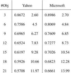
#Obj Yahoo Microsoft

3 0.8672 2.60 0.8986 2.70 6 0.7586 4.5 0.8069 4.84 9 0.6965 6.27 0.7609 6.85 12 0.6524 7.83 0.7277 8.73 15 0.6197 9.28 0.7026 10.54 18 0.5926 10.66 0.6823 12.28 21 0.5708 11.97 0.6661 13.99

Table 2.4: Compression ratio of denominator terms in Eqn. (2.3) in considering multiple ground-truth permutations.

In Section2.1.2, we introduce three strategies in selecting ground-truth permutations as model objective. The first one works well in Yahoo dataset, while it fails in Microsoft dataset: approximately 3 points in NDCG lower. The second one in PLRank(obj=1) works satisfactorily in terms of running time and performance. With respective to the third one, we locate an optimal setting to balance the running time and performance.

We empirically search an optimal setting to balance the running time and perfor-mance.Table2.4 displays actual compression ratio. For example, when objective number is 9, actual number of terms in computing the functional gradient is 69.6 percent of that without compressed storage, and this is equivalent to 6.27 objectives. From the results in

(50)

Tables2.3, 2.6, 2.4, we recommend to use PL(obj=3) in practice to gain stable improve-ments with acceptable extra training time.

2.2.4

PLRank vs.

l

-ListMLE, MART, McRank and LambdaMART

0.7000 0.7025 0.7050 0.7075 0.7100 0.7125 0.7150 0.7175 0.7200 0.7225 0.7250 Chart 13 NDCG@1 0 1 2 3 4 5 6 0.7000 0.7030 0.7060 0.7090 0.7120 0.7150 0.7180 0.7210 0.7240 0.7270 0.7300 Chart 14 NDCG@3 0.7650 0.7675 0.7700 0.7725 0.7750 0.7775 0.7800 0.7825 0.7850 0.7875 0.7900 Yahoo challenge 2010 Chart 15 NDCG@10 0.4510 0.4521 0.4531 0.4542 0.4552 0.4563 0.4573 0.4584 0.4594 0.4605 0.4615 Chart 16 ERR

PLRank(obj=1) PLRank(obj=3) PLRank(obj=6) 1 LambdaMART 2 McRank 4 MART-2 11 PL-linear

PLRank(obj=1) PLRank(obj=3) PLRank(obj=6) 1 LambdaMART 2 McRank 4 MART-2 11 PL-linear 0.7100 0.7109 0.7118 0.7127 0.7136 0.7145 0.7154 0.7163 0.7172 0.7181 0.7190 0 2 3 4 5 Chart 18 NDCG@1 0.7150 0.7161 0.7172 0.7183 0.7194 0.7205 0.7216 0.7227 0.7238 0.7249 0.7260 Chart 19 NDCG@3 0.7750 0.7764 0.7777 0.7791 0.7804 0.7818 0.7831 0.7845 0.7858 0.7872 0.7885

Yahoo Challenge with three-fold cross validation.

Chart 20 NDCG@10 0.4550 0.4553 0.4556 0.4559 0.4562 0.4565 0.4568 0.4571 0.4574 0.4577 0.4580 Chart 21 ERR

PLRank(obj=1) PLRank(obj=6) 1 LambdaMART

2 McRank 4 MART-2

PLRank(obj=1) PLRank(obj=6) 1 LambdaMART

2 McRank 4 MART-2 0.4900 0.4907 0.4914 0.4921 0.4928 0.4935 0.4942 0.4949 0.4956 0.4963 0.4970 0 1 2 3 4 5 Chart 4 NDCG@1 0.4770 0.4777 0.4784 0.4791 0.4798 0.4805 0.4812 0.4819 0.4826 0.4833 0.4840 Chart 5 NDCG@3 0.4980 0.4989 0.4998 0.5007 0.5016 0.5025 0.5034 0.5043 0.5052 0.5061 0.5070 Chart 6 NDCG@10 Microsoft 30K 0.3720 0.3726 0.3733 0.3739 0.3745 0.3752 0.3758 0.3764 0.3770 0.3777 0.3783 Chart 7 ERR

PLRank(obj=1) PLRank(obj=3) PLRank(obj=10) 1 LambdaMART 2 McRank 4 MART-2

Figure 2.3: Comparison of several tree-based systems.

(51)

Currently, the state-of-the-art learning to rank systems use boosted trees which have been proved to be more powerful than those using linear features in real world datasets. The champion of Yahoo challenge 2010 is a system that combines approximately 12 models, most of which are trained with LambdaMARTBurges et al.(2011). The other two state-of-the-art systems using trees are MART and McRank, one optimizes least-square loss and the other treat the ranking as a multi-class classification.

As shown in Table 2.3, PLRank outperforms l-ListMLE, which is a natural result

as PLRank is in a more complex function space than the linear space. However, what surprises us is that, in the Yahoo dataset there are moderate improvements, approximately 2 points in NDCG(@1, 3, 10), while in the Microsoft dataset, there are significant 8 to 10 points in NDCG(@1, 3, 10). On one aspect, boosted trees indeed could capture the dependency between features, and on another aspect, it is especially effective for the PL loss when the features are not rich.

As shown in Figure 2.3 and Table 2.3, the tree-based systems obviously perform well over linear feature systems. Among tree-based systems, PLRank demonstrates some moderate improvements over MART, McRank and LambdaMART in the Yahoo dataset, and in the Microsoft dataset, all tree-based systems perform pretty closely to each other.

McRank and PLRank are more close in six NDCG scores except NDCG@1 in the Microsoft dataset. LambdaMART performs well in ERR, and is significantly better than McRank and MART, and close to PLRank(obj=1). Comparatively, three PLRank variants act more stably. PLRank(obj=1) is always in best two systems on all measures when it is compared with McRank, on the other hand, as shown in Table 1 LambdaMART and MART. PLRank(obj=2) is considered to be the best in balancing the performance and

(52)

running time.

Two-tailed t-test results show PLRank(obj=*) systems would have significant im-provements over others when their differences are greater than about 0.5 point at 95% confidence. Unfortunately, in Table2.3, most of the improvements of PLRank(obj=*) are not significant, just matchable to these state-of-the-art systems.

Our MART baseline results are close to those reported inTyree et al.(2011). Tan et al.

Tan et al.(2013a) also used the same datasets to compare LambdaMART and MART, and

their baselines are about 1 point lower in NDCG than our reported results. We notice that their baselines are from RankLib, which is written in Java, and DirectRank is implemented in C++. In comparison, our 10 tree-based systems are re-implemented in C++ with an identical code template, thus our systems could be better to reflect differences in models rather than being impacted by coding.

2.2.5

PLRank vs.Other Consistent List-wise Method with Boosted

re-gression trees

The list-wise methods discussed in Section 2.1.5 have better performance than their in-consistent counterparts in Yahoo dataset, although the differences are not that much. In contrast, it is reported inRavikumar et al.(2011) that for all linear systems, the consistent versions improves NDCG scores of the in-consistent counterparts by several points.

As shown in Table 2.3, these consistent methods, after extended to boosted trees versions, unfortunately, have not show competitive performances when compared with LambdaMART, McRank and PLRank, so we did not run them on the larger Microsoft

(53)

dataset.

LambdaMART is a method that considers NDCG loss in optimization, and McRank optimizes unnormalized NDCG, so we only need to further analyze the surrogate functions of PLRank and the three consistent versions, that are not directly related to NDCG. A plausible explanation is the PL loss is consistent with NDCG@K, K taken 10, while

those of c-MART-1, c-CosMART, c-KLMART are consistent with NDCG with a whole list. We conjecture that when we letK go to the whole list, these systems would show

advantages.

2.2.6