Title Page
TRANSFER LEARNING FOR BAYESIAN CASE DETECTION SYSTEMS
by Ye Ye
Bachelor of Medicine, Peking University, 2006 Master of Science, Peking University, 2009
Master of Science in Public Health, Emory University, 2011
Submitted to the Graduate Faculty of
School of Computing and Information in partial fulfillment
of the requirements for the degree of Doctor of Philosophy
University of Pittsburgh 2018
Committee Membership Page
UNIVERSITY OF PITTSBURGH
SCHOOL OF COMPUTING AND INFORMATION
This dissertation was presented by
Ye Ye
It was defended on November 12, 2018
and approved by
Dr. Fuchiang Tsui, Associate Professor, Department of Biomedical and Health Informatics, Children's Hospital of Philadelphia
Dr. Michael M. Wagner, Professor, Intelligent Systems Program and Department of Biomedical Informatics, University of Pittsburgh
Dr. Gregory F. Cooper, Professor, Intelligent Systems Program and Department of Biomedical Informatics, University of Pittsburgh
Dr. Jeremy C. Weiss, Assistant Professor, Health Informatics at Heinz College, Carnegie Mellon University
Dissertation Director: Dr. Fuchiang Tsui, Associate Professor, Department of Biomedical and Health Informatics, Children's Hospital of Philadelphia
Dissertation Co-director: Dr. Michael M. Wagner, Professor, Intelligent Systems Program and Department of Biomedical Informatics, University of Pittsburgh
Copyright © by Ye Ye 2018
Abstract
TRANSFER LEARNING FOR BAYESIAN CASE DETECTION SYSTEMS Ye Ye, PhD
University of Pittsburgh, 2018
In this age of big biomedical data, a variety of data has been produced worldwide. If we could combine that data more effectively, we might well develop a deeper understanding of biomedical problems and their solutions. Compared to traditional machine learning techniques, transfer learning techniques explicitly model differences among origins of data to provide a smooth transfer of knowledge. Most techniques focus on the transfer of data, while more recent techniques have begun to explore the possibility of transfer of models. Model-transfer techniques are especially appealing in biomedicine because they involve fewer privacy risks. Unfortunately, most model-transfer techniques are unable to handle heterogeneous scenarios where models differ in the features they contain, which occur commonly with biomedical data. This dissertation develops an innovative transfer learning framework to share both data and models under a variety of conditions, while allowing the inclusion of features that are unique to and informative about the target context. I used both synthetic and real-world datasets to test two hypotheses: 1) a transfer learning model that is learned using source knowledge and target data performs classification in the target context better than a target model that is learned solely from target data; 2) a transfer learning model performs classification in the target context better than a source model. I conducted a comprehensive analysis to investigate conditions where these two hypotheses hold, and more generally the factors that affect the effectiveness of transfer learning, providing empirical opinions about when and what to share. My research enables knowledge sharing under heterogeneous scenarios and provides an approach for understanding transfer learning performance in terms of differences of features, distributions, and sample sizes between source and target. The
model-transfer algorithm can be viewed as a new Bayesian network learning algorithm with a flexible representation of prior knowledge. In concrete terms, this work shows the potential for transfer learning to assist in the rapid development of a case detection system for an emergent unknown disease. More generally, to my knowledge, this research is the first investigation of model-based transfer learning in biomedicine under heterogeneous scenarios.
Table of Contents
Preface ... xv
1.0 Introduction ... 1
1.1 Hypothesis Statement ... 3
1.2 Additional Research Questions ... 4
1.3 Contributions ... 7
1.4 Dissertation Organization ... 9
2.0 Background ... 10
2.1 Bayesian Case Detection System ... 10
2.2 Bayesian Network Learning ... 13
2.2.1 Bayesian Dirichlet Scoring Functions ... 14
2.2.2 Search Procedure ... 17
2.2.3 Some Bayesian Network Learning Algorithms ... 17
2.2.3.1 Naive Bayes ... 17
2.2.3.2 K2 ... 18
2.2.3.3 Efficient Bayesian Multivariate Classification Algorithm ... 19
2.3 Transfer Learning Techniques ... 21
2.3.1 Definition of Transfer Learning ... 21
2.3.2 Existing Transfer Learning Methods ... 22
2.3.2.1 Instance Weighting ... 22
2.3.2.4 Hyper-parameter Strategy ... 24
2.3.2.5 Model-Transfer ... 26
3.0 Bayesian Transfer Learning Framework ... 28
3.1 Summary of Notation ... 29
3.2 Identifying Different Types of Features ... 30
3.2.1 Information Gain Score ... 32
3.2.2 Correlation-based Feature Selection ... 33
3.3 BTLSD Algorithm ... 33
3.3.1 BTLSD-R: Weighting Based on Sample Size Ratio ... 34
3.3.2 BTLSD-KL: Weighting Based on Kullback-Leibler Divergence ... 34
3.3.3 BTLSD-FS-KL: Weighting Based on Feature-Specific KL ... 36
3.4 BTLSM Algorithm ... 37
3.4.1 Trimming the Source Model ... 37
3.4.2 Identifying Candidate Target-Specific Features ... 38
3.4.3 Conducting Recurring Grow-Prune Refinements ... 38
3.4.4 Proposed Score ... 39
3.4.5 Assigning Conditional Probabilities to the Selected Model Structure ... 43
3.4.6 An Illustration of BTLSM Algorithm ... 43
4.0 Evaluating the Transfer Learning Algorithms Using Synthetic Datasets ... 45
4.1 Experiment 1: Influenza Network ... 47
4.1.1 Experiment Design ... 47
4.1.2 Results Varying Source and Target Sample Sizes Across Six Transferring Scenarios ... 54
4.1.2.1 Source Size 8000, Target Size 50 ... 54
4.1.2.2 Source Size 8000, Target Size 8000 ... 56
4.1.2.3 Source Size 50, Target Size 50 ... 57
4.1.2.4 Source Size 50, Target Size 8000 ... 57
4.1.3 Discussion: Transfer Learning for Different Scenarios ... 78
4.2 Experiment 2: Intubation Network ... 80
4.2.1 Experiment Design ... 80
4.2.2 Results: Comparisons of Different Approaches for Empirical KL Divergence Estimation ... 84
4.2.3 Results: the Relationship between Transfer Learning and KL ... 86
5.0 Evaluating the Transfer Learning Algorithms Using Real-World Datasets ... 89
5.1 Datasets ... 91
5.2 Experiment Setting ... 94
5.3 Results: Influenza Detection among Suspected Visits ... 97
5.4 Results: Influenza Detection among General Emergency Room Visits ... 106
6.0 Discussion and Conclusions ... 113
6.1 Whether and When Transfer Learning Is Beneficial for the Target ... 113
6.2 Whether and When Transfer Learning Is Better Than the Source Model ... 116
6.3 Similarity Measurements for Transfer Learning Tasks ... 117
6.4 How Does the Target Data Size Impact the Effectiveness of Transfer Learning . 121 6.5 What Should Be Shared: Source Model or Source Data ... 121
6.6 Calibration Error Comparison ... 123
6.8 Conclusions ... 125
7.0 Contributions and Future Work ... 127
7.1 Contributions to Machine Learning ... 127
7.2 Contributions to Biomedical Informatics ... 129
7.3 Contributions to Disease Surveillance ... 130
7.4 Future Work ... 131
Appendix A Pseudocodes of BTLSD Algorithm ... 134
Appendix B Pseudocodes of BTLSM Algorithm... 139
List of Tables
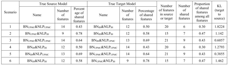
Table 1 Different types of features in transfer learning tasks ... 31 Table 2 Transfer learning scenarios and the difference between the target and the source ... 51 Table 3 Comparisons of mean AUC of models learned from 50-sample training datasets with different feature selection and machine learning algorithms ... 53 Table 4 Summative results for 10-fold experiments (source size=8000, target size=50) ... 58 Table 5 Average AUC and confidence interval of models in 10-fold experiments (source size=8000, target size=50) ... 59 Table 6 Average expected calibration error of models in 10-fold experiments (source size=8000, target size=50) ... 61 Table 7 Summative results for 10-fold experiments (source size=8000, target size=8000) ... 63 Table 8 Average AUC and confidence interval of models in 10-fold experiments (source size=8000, target size=8000) ... 64 Table 9 Average expected calibration error for models in 10-fold experiments (source size=8000, target size=8000) ... 66 Table 10 Summative results for 10-fold experiments (source size=50, target size=50) ... 68 Table 11 Average AUC and confidence interval of models in 10-fold experiments (source size=50, target size=50) ... 69 Table 12 Average expected calibration error for models in 10-fold experiments (source size=50, target size=50) ... 71 Table 13 Summative results for 10-fold experiments (source size=50, target size=8000) ... 73
Table 14 Average AUC and confidence interval of models in 10-fold experiments (source size=50, target size=8000) ... 74 Table 15 Average expected calibration error for models in 10-fold experiments (source size=50, target size=8000) ... 76 Table 16 Summary statistics of the differences between estimated KLs and true KLs in 705 runs ... 85 Table 17 Counts of encounters in IH and UPMC institutions ... 92 Table 18 Duration of outbreaks in IH and UPMC institutions ... 93 Table 19 Cumulative counts of IH and UPMC emergency room visits during 2014-15 influenza season. ... 94 Table 20 Classification performance when transferring knowledge from UPMC to IH for influenza detection among suspected visits ... 99 Table 21 Calibration performance when transferring knowledge from UPMC to IH for influenza detection among suspected visits ... 100 Table 22 Classification performance when transferring knowledge from IH to UPMC for influenza detection among suspected visits ... 101 Table 23 Calibration performance when transferring knowledge from IH to UPMC for influenza detection among suspected visits ... 102 Table 24 Features of models to detect influenza among suspected visits using first two weeks data ... 104 Table 25 Classification performance when transferring knowledge from IH to UPMC for influenza detection among emergency department visits ... 108
Table 26 Calibration performance when transferring knowledge from IH to UPMC for influenza detection among emergency department visits ... 109 Table 27 Classification performance when transferring knowledge from UPMC to IH for influenza detection among emergency department visits ... 111 Table 28 Calibration performance when transferring knowledge from UPMC to IH for influenza detection among emergency department visits ... 112 Table 29 KL between target and source distributions in datasets of UPMC and IH ... 119
List of Figures
Figure 1 Types of features in the source and the target (Red box: features in the source model.
Green box: features in the target model) ... 30
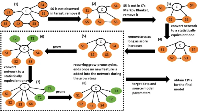
Figure 2 An illustration of the BTLSM algorithm ... 44
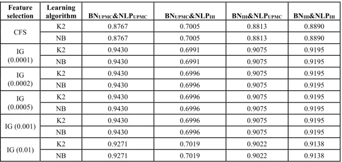
Figure 3 Four Bayesian network models developed using datasets distinguished by data resources (i.e., IH notes or UPMC notes) and NLP parsers (i.e., IH parser or UPMC parser) (from Ye et al. 2017) ... 49
Figure 4 Comparison of feature spaces of the source model and the target model between scenario 1 and 4 ... 79
Figure 5 Intubation network (a subgraph of the ALARM network, (Beinlich et al. 1989)) ... 82
Figure 6 Performance changes at different rates when KL increases (feature selection=CFS, source size=8000, target size=50) ... 87
Figure 7 Performance changes at different rates when KL increases (feature selection=information gain with threshold 0.0001, source size=8000, target size=50) ... 88
Figure 8 Three types of outbreak timelines in two regions ... 90
Figure 9 Seven-day average counts of lab-confirmed cases in IH and UPMC ... 93
Figure 10 BTLSM approach used in the real-world influenza experiment ... 96
List of Equations Equation 1 ... 5 Equation 2 ... 5 Equation 3 ... 15 Equation 4 ... 18 Equation 5 ... 20 Equation 6 ... 35 Equation 7 ... 35 Equation 8 ... 36 Equation 9 ... 39 Equation 10 ... 40 Equation 11 ... 40 Equation 12 ... 40 Equation 13 ... 40 Equation 14 ... 42 Equation 15 ... 42 Equation 16 ... 43 Equation 17 ... 54 Equation 18 ... 83
Preface
The PhD study in University of Pittsburgh is an adventure for me. This journey would not have been possible without the support of my family, friends, and professors. I would like to thank my advisor, Dr. Fuchiang Tsui, who introduced me to the Intelligent System Program, guided me all the way through the adventure, and provided me great insight into research question development, study design, and software engineering. I would like to give special thanks to my cochair, Dr. Wagner, who led me towards the path of artificial intelligence for population health, believed my potential in population health informatics, and always supported me to pursue my career. I deeply appreciate the support from my committee, Dr. Cooper, who showed me the most rigorous science, and was always available for research discussions, career advice, and recommendations. I would like to thank my committee, Dr. Weiss and Dr. Day, for their supports on study design and theoretical foundations. I would like to thank the ISP and DBMI program to design the medical informatics track, which is a bridge between artificial intelligence and biomedicine. I learned theoretical foundations and scientific thinking from Drs. Weibe, Hwa, and Litman. I appreciate Dr. Becich’s guidance and insights. He is a great coach for DBMI students. I enjoy working in the RODS lab and have learned a lot from John Arnois, Espino, Nick, and John Levander. Our Utah collaborators, Drs. Haug, Ferraro, and Gesteland provided massive high-quality research data, with which I get hands dirty. I would like to thank Dr. Druzdzel and BayesFusion Company to provide JSMILE engine for Bayesian inference in my study. I received a lot of support from Cleat, Howard, Toni, Michele, Lucy, Rob, and Jesse. I would like to thank Yun and Jannie for reviewing my dissertation. My friends and classmates (Yun, Kevin, Yuriy,
provided technique advice. I would especially like to thank my family, my father, Zhonghua, my mother, Yanghua, my younger sister, Yunhan, my husband, Diyang, my mother-in-law, Xiaofang, my father-in-law, Xiaoyong, and my lovely baby, Jane, for unconditional love and support.
1.0Introduction
In the age of big biomedical data, massive amounts of digital biomedical data have been produced worldwide. If we were able to better integrate data/knowledge from all possible resources, then a deeper understanding of biomedical phenomenon would be possible.
Although many traditional machine learning technologies have been successfully used for knowledge discovery from biomedical data, the discovered knowledge may be not ready for applying to different regions, hospitals, or laboratories. Traditional machine learning technologies usually work under the assumption that the data for model development and the data for model deployment later have the same underlying distribution. This assumption is sometimes too strict if the training and test are from different regions/hospitals. The test data could have a different set of features from the training data. Even if the training and test data have a same set of features, the correlation between predictive features and class variable could be different between training data and test data. When applying a model developed with training data to the test data, their differences could lead to a dramatic performance drop.
On the other hand, there is a need to borrow/learn knowledge from other regions, hospitals, or laboratories. Retraining a model from scratch using target data could be expensive and sometimes infeasible. There may be insufficient historical data available from the target area. Also, the amount of labeled target data for supervised machine learning may be inadequate.
The goal of transfer learning is to provide a smoother transfer of knowledge from the source to the target, which is similar but not identical to the source. Transfer learning algorithms (Lu et al. 2015) consider both the similarities and the differences between the source and the target.
Transfer learning could be a key way to increase the effectiveness of worldwide disease surveillance. The ability to predict, forecast, and control disease outbreaks highly depends on the ability of disease surveillance. Compared to traditional laboratory reporting and physician reporting system, automated case detection based on electronic medical records has much less time delay and may cover a large population. However, development of an automated case detection system may require a large training dataset for modeling, but not all regions have it. One solution is that, when region A were affected by an outbreak first, it could share its developed case detection system to region B before region B was significantly affected. Since both regions cover different populations that are served by healthcare institutions with different electronic medical record systems, their features and distributions for case detection could be different. These differences usually lead to a dramatic performance drop. When region B has a few cases, with these cases, transfer learning techniques could adapt a case detection system from region A with data pattern in region B and thus increase the case detection capability for region B.
Similarly, transfer learning will help enhance the capabilities of nationwide collaborations in secondary use of electronic medical records (Chute et al. 2011), patient-centered outcome research (Selby et al. 2012), and observational scientific research (Hripcsak et al. 2015).
1.1Hypothesis Statement
This dissertation aims to develop and evaluate a transfer learning framework for case detection using Bayesian networks over discrete variables following multinomial distributions. The developed framework (Chapter 3) is able to conduct transfer learning in two different scenarios: (1) source data and target data are available, (2) source model and target data are available.
I tested two hypotheses. Hypothesis 1: a transfer learning model that is learned using source knowledge and target data performs classification in the target context better than a target model that is learned solely from target data. This hypothesis is explored under several conditions that vary with respect to the degree of difference in features, distributions, and sample sizes in the source and the target contexts. To test this hypothesis, I compared the discriminative ability of a target model developed with the target data only, with the discriminative ability of another target model developed with both the target data and the source data (or the source model) using the proposed transfer learning algorithms. To evaluate model performance, I used a set of target instances that have not been used for model development, measuring each model’s discriminative ability for the classification task.
The second hypothesis tested is that a transfer learning model learned using source knowledge and target data performs classification in the target context better than a source model that was learned in the source context. This hypothesis is explored under several conditions, including those in which (1) the source and target distribution differences are relatively large and there is a need to adjust the transferred source model, and (2) the target training data are large enough to adjust the target model to the target context. To test this hypothesis, I compared the
discriminative ability of a source model with the discriminative ability of a target model developed with both the target data and the source data (or the source model).
1.2Additional Research Questions
To clearly define the conditions of the hypotheses and better understand the conditions where transfer learning improves over conventional machine learning methods, I explored three additional research questions: (1) how does similarity between the source and the target relate to the transfer outcomes (positive or negative)? (2) How does the target data sample size affect the effectiveness of transfer learning? (3) What should be shared, source model or source data, and when?
Question (1): How does similarity between the source and the target relate to the transfer outcomes?
Transfer learning aims to transfer knowledge from the source to the target. However, not every transfer is beneficial for the target. When the two domains are very different (e.g., few generalizable features, completely different distributions), transfer learning could be unnecessary or even harmful (i.e., negative transfer).
The study of the relationship between similarity of domains and the effect of transfer learning could provide insight into how to avoid worthless or negative transfer. In my study, similarity between the two domains is measured using two indicators: (1) the KL divergence between the distributions of the two domains (Eq. 1), which penalizes the situation when 𝑃𝑃(𝑖𝑖) is
large and 𝑄𝑄(𝑖𝑖) is small, and (2) the proportion of overlapping features among all features (POF) from both domains (Eq. 2).
Equation 1
𝐾𝐾𝐾𝐾(P|| Q) =∑iP(i) ×Q(i)P(i)
where 𝑃𝑃(𝑖𝑖) and 𝑄𝑄(𝑖𝑖) are joint probability distributions for the ith configuration of feature values.
Equation 2
𝑃𝑃𝑃𝑃𝑃𝑃 = 𝑁𝑁𝑁𝑁𝑓𝑓∈�𝐹𝐹𝑆𝑆∩𝐹𝐹𝑇𝑇�
𝑓𝑓∈�𝐹𝐹𝑆𝑆∪𝐹𝐹𝑇𝑇�
where 𝑃𝑃𝑆𝑆 represents the feature set of the source data, and 𝑃𝑃𝑇𝑇 represents the feature set of the target data.
The effect of transfer learning is indicated by the difference between the performance of a target model developed with both the target data and the source data (or the source model) and the performance of a target model developed with only the target data. If a transferred model performs significantly better than a local model in testing target instances, then the transfer is positive. If a transferred model performs significantly worse than a local model in testing target instances, then the transfer is negative. If the two models perform similarly, then the transfer is unnecessary.
The relationship between similarity of domains and the effect of transfer learning may depend on the number of instances of the target data. When the target has sufficient data to develop a reliable local model, transfer learning may become unnecessary even if source and target distributions are identical.
This dissertation investigates these relationships in synthetic experiments (Chapter 4) and real-world experiments (Chapter 5).
Question (2): How does the target data sample size impact the effectiveness of transfer learning? Target models with more features and/or greater complexity usually require a larger training sample in order to learn a model. In other words, similarity between the two domains and complexity of the underlying target model impact how large a target dataset is required to learn a model. If the two domains are very different, a transferred model may not perform better than a less reliable model developed with a few target instances.
To study the effects of target sample size on the effectiveness of transfer learning, I generated synthetic datasets with different target sample sizes (Chapter 4). I also assessed different timelines in real-world datasets, which corresponds to different sizes of target training data (Chapter 5).
Question (3): What should be shared, source model or source data, and when?
Although sharing a model is more feasible than sharing data, researchers may still have concerns about information loss.
The comparison between the effects of sharing a source model and the effects of sharing source data under different transfer learning tasks (Chapter 4 and 5) varying for degree of feature space overlapping, similarities of distributions, and sample sizes provides insight into the critical questions in biomedical knowledge sharing of what to share and when.
1.3Contributions
This dissertation develops a framework for transfer of knowledge (in the form of a model) across institution boundaries in heterogeneous scenarios (feature space differences and distribution differences). I developed an innovative score for model searching, which considers both source model information (structure and conditional probabilities) and the data pattern (correlations between features and class variables) in the target domain. The score allows for features that were measured in the target domain but not in the source domain, making the localization of a transferred model more flexible for heterogeneous scenarios.
To my knowledge, the developed algorithm is the first transfer learning algorithm for Bayesian network transfer for heterogeneous scenarios. Compared to another linear SVM based model-transfer technique for heterogeneous scenarios (Mozafari et al. 2016), my algorithm does not require relatively large target sample for target model development, while at the same time integrating much more parameter information from the source model rather than just using a one-dimensional offset parameter from the source model. It has fewer restrictions than other algorithms as well: it neither assumes linear correlations between features and the classification task, nor assumes a very similar feature distribution in a transformed common dimension. Compared to popular deep transfer learning techniques, my algorithm does not require a large number of target samples for model tuning, and it can handle the feature space difference issue that is not rare in machine learning tasks and also is very common in medical data. Compared to traditional transfer learning techniques, my algorithm does not necessarily need to use original source data, which makes model reuse an appealing alternative for knowledge sharing.
the algorithm does not require a prior network to cover all predictive features, and it allows different levels of confidence for different features. These extensions make model learning more flexible and reliable.
I conducted a comprehensive analysis in both synthetic datasets and real-world datasets to investigate critical questions about transfer learning tasks: when to share and what to share (model or data). I recommended four measurements to estimate the success of transfer learning: percentage of shared features among all features, percentage of shared features among target features, average KL divergence, and performance of source model on target data. When the target domain has few samples, sharing the source model was found to archive a performance comparable to that of sharing the source data. When the target domain has many samples, sharing the source data was more flexible for knowledge discovery.
In addition, to my knowledge, this is the first study of model transfer using biomedical data in heterogeneous scenarios. The results demonstrate an impact of task similarity on the success of transfer learning; therefore, I recommend a well-established terminology standard and a generalizable natural language processing parser to enhance knowledge sharing for biomedical research.
Also, this is the first study on transfer learning techniques for infectious disease detection tasks. This dissertation demonstrates the transferability of case detection systems and shows the benefits of sharing in the early stage of outbreaks. Using influenza as a proxy for an emergent unknown disease, it demonstrates the possibility of quickly developing a high-performance case detection system that uses natural language processing to extract clinical findings (features) from routinely collected emergency room reports.
1.4Dissertation Organization
The rest of the dissertation is organized as follows. Chapter 2 provides transfer learning and offers a review of transfer learning techniques in two categories: data transfer (instance weighting, feature representation, self-labeling, and hyper-parameter), and model transfer. Chapter 2 then describes the design of my Bayesian case detection systems. Chapter 3 explains the developed transfer learning framework, including description of Bayesian transfer learning using the source data algorithm (BTLSD) and Bayesian transfer learning using the source model algorithm (BTLSM). Chapter 4 presents the experimental results of the proposed algorithms on synthetic datasets and Chapter 5 presents the experimental results on real-world datasets. Chapter 6 summarizes the research findings and discusses the dissertation hypotheses in light of the results obtained. Finally, Chapter 7 summarizes the contributions and discusses future lines of research.
2.0Background
This Chapter provides an introduction of Bayesian case detection system, Bayesian network learning, and current transfer learning techniques.
2.1Bayesian Case Detection System
The control of epidemic diseases is an increasingly important global problem. The spread of an infectious disease could be very fast in a dense population with low immunity levels. The increasing incidence of domestic and international travel further hastens the speed of contamination. In in multi-region epidemics, efficient and effective infectious disease control strategies strongly rely on the capability of disease surveillance, which must be amenable to widescale rapid deployment.
Traditional case detection mainly relies on notifiable disease reporting and sentinel physician systems; however, issues with time delay and underreporting often occur. As a result, substantial investment and research has been put into public health to include automated surveillance that leverages routinely collected electronic information such as laboratory test orders and results (Panackal et al. 2002, Overhage et al. 2008), chief complaints (Ivanov et al. , Espino et al. 2001, Wagner et al. 2004, Chapman et al. 2005), sales of over-the-counter medications (Wagner et al. 2004, Rexit et al. 2015), and encounter notes (Elkin et al. 2012, Gerbier-Colomban et al. 2013).
Since 2011, our research lab has been developing a type of Bayesian case detection system (BCD) as part of a probabilistic framework for case and outbreak detection (Tsui et al. 2011, Wagner et al. 2011, Cooper et al. 2015). This system uses natural language processing (NLP) to infer the presence or absence of clinical findings from narrative notes. With these findings, a Bayesian network model infers each patient’s diagnosis probabilities. The BCD also provides the likelihood of patient clinical evidence supporting outbreak detection and prediction at the population-level. We chose Bayesian network models because they separately represent prior probability of the diagnosis (i.e., P(diagnosis)) and likelihood of clinical findings (i.e., P(clinical
findings | diagnosis)). This representation allows our outbreak detection algorithms (Cooper et al.
2015) to use dynamic priors for the diagnosis node, which reflects the changing prevalence of disease during an outbreak.
The initial focus of the disease surveillance was influenza, which was fielded in Allegheny County, PA in 2009. We showed that our influenza case detection system performed well in the location in which it was built (Tsui et al. 2011, López Pineda et al. 2015). For the input of a case detection system, another researcher, Elkin first showed that using whole encounter notes was more accurate for case detection than using only the chief complaint field (Elkin et al. 2012). Ruiz’s study found the benefit of using multiple clinical notes associated with an encounter (Ruiz 2014). For the NLP component of the case detection system, I compared performance of BCD using human annotated findings with performance using NLP extracted findings, and found that the latter led to a drop in AUC of about 0.06 (Ye et al. 2014).
We also conducted three studies that analyzed the Bayesian network model component. The first study (Ye et al. 2014) showed that feature selection increases performance. Specifically, models using a subset of findings had better performance than models using a full set of findings.
Although the full set of findings had been defined by experts, NLP extraction changed the strength of associations between many clinical findings and diagnosis. The second study (López Pineda et al. 2015) showed that machine learning alone was as good as a combination of expert knowledge and machine learning, thus providing support that we might be able to eliminate a labor-intensive development step. The third study (Tsui et al. 2017) showed that using the actual dynamic prior of diagnosis could increase the discriminative ability of an influenza detection model comapred to using a constant diagnosis prior.
Overall, effective and efficient management of disease outbreaks would benefit from automated case detection systems such as those described above that can be rapidly deployed across institutional and geographical boundaries. For example, my recent research about transferability demonstrated high influenza case detection performance in two large healthcare systems in two geographically separate regions, the University of Pittsburgh Medical Center (UPMC) and the Intermountain Healthcare (IH) System in Utah, providing support for the use of automated case detection from routinely collected electronic clinical notes in national influenza surveillance (Ye et al. 2017). In addition, I identified the influence of natural language processing on transferability. However, for a BCD developed with IH training data experienced reduced performance. We attribute this to the lower recall of an IH natural language processing parser on the UPMC notes, from which the section-specific rules in IH parser failed to extract influential findings.
These results indicate that case detection using NLP-extracted clinical findings may encounter transferability challenges. NLP-extracted findings of clinical notes from different institutions may have different feature sets with different distributions. Most medical NLP parsers (Friedman et al. 2004, Harkema et al. 2009, Savova et al. 2010)rely on rule-based processing
engines, which rules are usually manually built by knowledge engineers based on expert-annotated sample clinical notes from one institution. It is difficult to automatically refine these rules for another institution. Moreover, different institutions may have different templates in their electronic medical record systems and their clinicians may also write notes differently. Therefore, it is very common that NLP-extracted findings of clinical notes from different institutions have different feature sets with different distributions. Transfer learning of Bayesian network models could thus be helpful.
2.2Bayesian Network Learning
To increase the transferability of case detection systems, my dissertation study focuses on transfer learning for Bayesian network models. The Bayesian network models represent the uncertainty of a disease using probabilistic graphic models. Typically, the structure of the models represents the correlations between clinical findings and diseases. Their strength is represented by a set of conditional probability tables. Both the structure and the parameters of a Bayesian network model can be automatically induced from data by machine learning algorithms.
Learning a Bayesian network model usually involves both structure learning and parameter learning. Learning Bayesian network structures is NP-hard (Chickering et al. 1994). Three strategies have been used for machine learning: a score-and-search approach, a constraint-based approach, and a dynamic programming approach (Daly et al. 2011), which is a score-based approach without search procedure.
knowledge. Many score-based structure-learning algorithms estimate parameters as part of the scoring process. When calculating a score, an implicit parameterization is always given. The parameter learning is usually a subroutine in structure learning. For Bayesian scores, there is usually not a single parameterization, but rather all possible parameterizations are considered by integrating over them and using a parameter prior while doing so.
The constraint-based approach constructs a dependency structure based on conditional independencies identified by statistical tests on the data. While the score-and-search approach usually works better with less data and with probability distributions with dense graphs and is able to represent probability distributions easily (Daly et al. 2011), the constraint-based approach is typically quicker and is good at modeling hidden common causes and selection bias (Daly et al. 2011).
The dynamic programming approach uses dynamic programming to compute optimal models for a small set of variables (no larger than 30) (Daly et al. 2011). It is similar to the score-and-search approach but performs an exhaustive search.
My proposed transfer learning algorithms uses the Bayesian Dirichlet scoring function and a local search approach, described below.
2.2.1 Bayesian Dirichlet Scoring Functions
Bayesian Dirichlet scoring functions usually compute the relative posterior probability of each candidate network-structure hypothesis given data and prior knowledge, assuming multinomial distributions on the data, parameter independence, parameter modularity, a Dirichlet distribution to represent the parameter priors, and complete independent and identically distributed
The Parameter independence assumption includes global and local independence. Global independence means that parameters associated with each node in a network are independent, while local independence means that parameters associated with each state of the parents of a node are independent. With these independence assumptions, I can transform the probability density of all parameters into the multiplication of the individual probability density of each parameter that is associated with each state of the parents of a node. These independence assumptions make the score decomposable: the score of a network structure is the product of the score of each node given its parents.
The parameter modularity assumption assumes identical probability density functions of parameters associated with a node in two distinct networks if the node has the same parents in those two networks.
The assumptions of parameter independence and parameter modularity make the comparison between two different network structures more efficient, enabling a focus solely on those nodes that have different parents in two network structures.
The Dirichlet assumption means that prior parameters associated with each state of the parents of a node follow a Dirichlet distribution.
Under these assumptions, the joint probability of a network structure 𝐵𝐵𝑆𝑆ℎ and data D can be calculated as shown in Eq. 3 (Heckerman et al. 1995):
Equation 3 𝑝𝑝�𝐷𝐷,𝐵𝐵𝑆𝑆ℎ�𝜉𝜉�= 𝑝𝑝�𝐵𝐵𝑆𝑆ℎ�𝜉𝜉� ∏ ∏ 𝛤𝛤(𝑁𝑁𝑖𝑖𝑖𝑖 ′) 𝛤𝛤(𝑁𝑁𝑖𝑖𝑖𝑖′+𝑁𝑁𝑖𝑖𝑖𝑖) 𝑞𝑞𝑖𝑖 𝑗𝑗=1 𝑛𝑛 𝑖𝑖=1 ∏ 𝛤𝛤(𝑁𝑁𝑖𝑖𝑖𝑖𝑖𝑖 ′ +𝑁𝑁 𝑖𝑖𝑖𝑖𝑖𝑖) 𝛤𝛤(𝑁𝑁𝑖𝑖𝑖𝑖𝑖𝑖′ ) 𝑟𝑟𝑖𝑖 𝑘𝑘=1
The term 𝑁𝑁𝑖𝑖𝑗𝑗𝑘𝑘′ denotes prior parameters of the Dirichlet distribution, where the prior probability of one configuration of parameters is the product of these parameters powered by the
a user’s prior knowledge about the model. For the special case when 𝑁𝑁𝑖𝑖𝑗𝑗𝑘𝑘′ =1, the BD measure is the K2 measure (Cooper et al. 1992).
Another example of a BD measure is the Bayesian Dirichlet likelihood equivalent (BDe) measure (Heckerman et al. 1995). The BDe measure is a likelihood-equivalent Bayesian scoring metric. The likelihood-equivalence assumption assumes that network structures representing the same assertions of conditional independence have the same likelihood. The assumptions of likelihood equivalence and parameter independence imply that the parameter priors must follow a Dirichlet distribution (Heckerman et al. 1995).
The definition of the BDe measure is given in (Heckerman et al. 1995): Given a domain U of n discrete variables x1, …, xn, suppose that prior distribution ρ(ΘU|𝐵𝐵𝑆𝑆𝑆𝑆ℎ ,ξ) is Dirichlet with prior
equivalent sample size 𝑁𝑁′ for network structure BSC in U. Then, for any network BS in U, assumptions of a multinomial sample, parameter independence, parameter modularity, complete data, and structure possibility, imply 𝑁𝑁𝑖𝑖𝑗𝑗𝑘𝑘′ =𝑁𝑁′p(𝑥𝑥𝑖𝑖 = k,𝜋𝜋𝑖𝑖 = j|𝐵𝐵𝑆𝑆𝑆𝑆ℎ ,ξ). In situations with uniform joint distribution constraint (i.e., all configurations have same probabilities), 𝑁𝑁𝑖𝑖𝑗𝑗𝑘𝑘′ can be calculated as 𝑟𝑟𝑁𝑁′
𝑖𝑖𝑞𝑞𝑖𝑖. The BDe with this assignment is called BDeu (Bayesian Dirichlet with likelihood
equivalence and a uniform joint distribution) (Daly et al. 2011).
Since the variance of the parameters is proportional to 1/𝑁𝑁′, the prior equivalent sample size reflects a user’s confidence for the prior network. Thus, 𝑁𝑁′ can be assessed as the number of observations that would have been seen in order to have the same confidence as a prior knowledge. Using simulation data generated by a gold-standard network, (Heckerman et al. 1995) studied the behavior of a learning Bayesian network initiated using a prior network, and found that the optimal equivalent sample size for a prior network decreases as the difference in distributions between the
2.2.2 Search Procedure
For tree-like Bayesian networks (every node has at most one parent), the search for the network structure with the highest score is a “finding maximum branching” problem, which can be solved in polynomial time (Karp 1971, Gabow et al. 1984). When the score assumes likelihood equivalence, a maximum spanning tree algorithm can identify the undirected forest with the highest score, followed by adding any directionality to the arcs to obtain a collection of equivalent network structures.
When allowing some nodes to have more than one parent, the search for the network structure with the highest score is NP-hard (Heckerman et al. 1995). One simple heuristic search algorithm is a local search, which makes the most valuable change (measured by score) at each move in the search process until no change leads to an increase of score. The local search approach is relatively fast when using a decomposable measure (e.g., BD metric), because this type of measure allows us to avoid re-computing all terms after every change. One potential problem with a local search is that it may get struck at a local maximum. To avoid this problem, I can use an iterated local search or simulated annealing. Compared to random initiation, prior structure knowledge is found to be more useful for initiating a local search (Heckerman et al. 1995).
2.2.3 Some Bayesian Network Learning Algorithms
2.2.3.1Naive Bayes
The Naïve Bayes algorithm assumes conditional independence of predictive nodes given the class node. This assumption dramatically simplifies the structure of a Bayesian network: arcs
reduces the number of parameters (i.e., conditional probabilities) from exponential to linear in the number of nodes.
The conditional probabilities of a Naïve Bayesian network can be estimated using either maximum likelihood estimates or maximum a posterior (MAP) estimates (Mitchell 1997). One potential problem with the maximum likelihood approach is that the estimated conditional probability will be 0 if a particular event does not appear in the training data. This is common when the training data has a small sample size. The MAP approach uses prior distributions to smooth the parameter estimation. Eq. 4 shows Laplace smoothing.
Equation 4
𝑃𝑃 (𝑋𝑋𝑗𝑗 = 𝑥𝑥𝑗𝑗𝑘𝑘 | 𝑌𝑌 = 𝑦𝑦𝑚𝑚) =∑ 𝐼𝐼(𝑋𝑋 ∑ 𝐼𝐼( 𝑌𝑌 = 𝑦𝑦𝑖𝑖 = 𝑥𝑥𝑖𝑖𝑖𝑖, 𝑌𝑌 = 𝑦𝑦𝑚𝑚) + 𝑟𝑟𝑚𝑚𝑖𝑖)+ 1
The performance Naïve Bayes algorithm has been shown to be comparable to much more complicated models (Domingos et al. 1997). Although the traditional Naïve Bayes learning algorithm does not conduct any feature selection, it is usually very robust against overfitting in terms of discrimination. However, it is sensitive to strong correlations between features that violate the conditional independence assumption. Inference on a Naïve Bayesian network is computationally easy, but the posterior probabilities are usually not well calibrated: they are too close to 0 or 1 (Zadrozny et al. 2001).
2.2.3.2K2
The Naïve Bayes algorithm has a conditional independence assumption, which may not be able to represent the complicated correlations between variables in biomedical data. After relaxing this assumption, in order to find the most probable network structure in a polynomial time, many Bayes learning algorithms use some restrictions and assumptions to reduce the search space.
The K2 algorithm (Cooper et al. 1992) assumes a uniform prior over structures, and requires input of an ordering of the candidate variables and the maximum number of possible parents. Starting from an empty Bayesian network, the algorithm incrementally adds the parents of nodes as long as the addition increases the K2 score. Candidate parents of a node are restricted by the ordering of the candidate variables. Only variables proceeding a variable in the ordering can be considered as candidates of parents. The number of parents of a node is also restricted by the maximum number of possible parents.
The complexity of the K2 algorithm is O (mn4r), where m is sample size of the training
data, n is the size of the feature space, and r is the maximum number of possible values for any variable.
2.2.3.3Efficient Bayesian Multivariate Classification Algorithm
The above two algorithms do not conduct feature selection. The efficient Bayesian multivariate classification algorithm (EBMC) (Cooper et al. 2010) was developed to efficiently identify a Bayesian network that predicts a target variable.
EBMC conducts a greedy forward-stepping search. The search starts from an empty model and conducts recurring grow-and-prune cycles. During a growth phrase, EBMC uses a score to add the single best predictive node as a parent of the class node. After that, EBMC continuously adds parent nodes of the class node as long as the addition increases the score. When no additional node improves the score, EBMC starts a pruning phase. It converts the Bayesian network into a statistically equivalent Bayesian network that has the same score. Then, EBMC searches for an arc such that removing the arc increases the score the most. It keeps removing arcs until no single arc removal would increase the score. When the pruning phase stops, the search starts a new
grow-the score in grow-the growth phrase. In this way, EBMC finds a high-scoring Markov blanket Bayesian network of the class node.
The score in EBMC uses a supervised (prequential) scoring. It also uses the BDeu strategy to incorporate prior knowledge through a prior equivalent sample size parameter. A structure prior of a candidate model in the EBMC search are estimated using a binomial distribution, and it is the product of the probability of including predictive variables in the model and the probability of excluding other variables as candidate predictors (Eq. 5, which is from (Cooper et al. 2010, Jiang et al. 2014),
Equation 5
𝑃𝑃𝑃𝑃𝑖𝑖𝑃𝑃𝑃𝑃= 𝑝𝑝𝑁𝑁𝑃𝑃+𝑁𝑁𝐶𝐶× (1− 𝑝𝑝)𝑁𝑁−(𝑁𝑁𝑃𝑃+𝑁𝑁𝐶𝐶)
where p is the probability of including any given predictor in the model, and it is estimated as the ratio between the expected number of predictors and the total number of candidate predictors. 𝑁𝑁𝑃𝑃 is the number of parents of the outcome node, 𝑁𝑁𝑆𝑆 is the number of children of the outcome node. The prior is a product of the probability of each predictor in the model, and that probability is estimated using the proportion of expected number of predictors of the class node.
The complexity of an EBMC search is O (rs2mn), where r is the total number of children
node clusters, s is the maximum size of parents of the class node, n is the size of the feature space, and m is the size of the training data.
EBMC has been used to predict clinical outcomes from genome-wide data (Cooper et al. 2010, Jiang et al. 2014), and to detect influenza from emergency department free-text reports (López Pineda et al. 2015). In the studies performed to date, EBMC often has the predictive performance comparable to other traditional machine learning approaches while taking less time to learn a model.
2.3Transfer Learning Techniques
In this section, I provide a definition of transfer learning, and then introduce five different transfer learning strategies.
2.3.1 Definition of Transfer Learning
(Pan et al. 2010) gave a definition of transfer learning as follows: “Given a source domain
DS and learning task TS, a target domain DT, and learning task TT, transfer learning aims to help
improve the learning of the target predictive function (target model) fT(.) in DT using the knowledge
in DS and TS, where DS≠ DT, or TS≠ TT.” In this definition, a domain is denoted by D = {χ, P(X)},
where χ is the feature space, and P(X) is the marginal probability distribution of features. A task
is denoted by T={Y, f(.)}, where Y is the label space of the class variable, and f(.) is an objective predictive function to be learned.
The main difference between a transfer learning problem and a traditional machine learning problem is whether the source and the target have an identical domain and task. In the definition of transfer learning, the source and the target may have different but related domains or have different but related tasks. Most transfer learning studies only focus on transfer learning tasks under one condition (i.e., domains are different, but tasks are identical; or domains are identical, but tasks are different).
2.3.2 Existing Transfer Learning Methods
Transfer learning techniques aim to provide a smoother transfer of knowledge in the form of models from the source to a different but related target. Existing transfer learning techniques can be divided into two branches: data transfer and model transfer. Data transfer includes four main categories: instance weighting (Huang et al. 2006, Jiang 2008, Sugiyama et al. 2008), feature representation (Aue et al. 2005, Arnold et al. 2007, Jiang et al. 2007, Satpal et al. 2007, Ciaramita et al. 2010, Pan et al. 2010, Pan et al. 2011, Wiens et al. 2014, Ogoe et al. 2015), self-labeling (Dai et al. 2007, Tan et al. 2009), and the hyper-parameter strategy (Roy et al. 2007, Finkel et al. 2009).
2.3.2.1Instance Weighting
In order to adjust for difference between the marginal distribution of the source and of the target, some transfer learning algorithms assign different weights to instances from the two resources.
Jiang (Jiang 2008) represented a classification problem in the transfer learning setting as an optimization problem, with the aim of finding an optimal solution that minimized the expected loss with respect to the distribution of the target. The optimization process involved assigning different weights to instances from the source and the target in order to adjust the estimated loss. For each instance (𝒙𝒙𝒊𝒊,𝑦𝑦𝑖𝑖) in the source, the suggested weight was PPst(𝑦𝑦(𝑦𝑦𝑖𝑖𝑖𝑖| 𝒙𝒙| 𝒙𝒙𝒊𝒊𝒊𝒊)) , which was the ratio between the conditional probability in the target data and the conditional probability in the source data. For each labelled instance in the target, the suggested weight was the ratio between the number of instances in the source and the number of labelled instances in the target.
Other approaches aim to increase the similarity between the source and target distributions. To reweight instances in the source, Huang et al. (Huang et al. 2006) proposed a kernel mean matching approach, and Sugiyama et al. (Sugiyama et al. 2008) proposed a Kullback-Leibler importance estimation procedure.
2.3.2.2Feature Representation
Many transfer learning algorithms manipulate features to maximize the similarity between the source and the target distributions. Two strategies (Weiss et al. 2016) may be utilized to maximize the similarity: (1) asymmetric transformation of the source domain to the target domain, (2) symmetric transformation mapping of the source and target domains into a common feature space.
Asymmetric transformation aims to transform features in the source to be similar to features in the target. For example, Wiens et al. (Wiens et al. 2014) conducted two transformations for source data: (1) remove source-specific features, (2) map source data to the target feature space by augmenting with zeros. Other distribution similarity approaches (Aue et al. 2005, Arnold et al. 2007, Jiang et al. 2007, Satpal et al. 2007) penalize or remove features whose distributions are different in the source and the target.
Symmetric transformation aims to map the source and target domains into a common feature space. For example, latent feature methods construct new features by analyzing large amounts of unlabeled source and target data (Ciaramita et al. 2010, Pan et al. 2010). Ogoe et al. (Ogoe et al. 2015) implemented a gene ontology-similarity-based method to identify common variables in the source and target datasets. Using this functional mapping, the performance of their transfer rule learner was improved and was shown to perform better than other integrative models
based deep learning algorithms (Ajakan et al. 2014, Long et al. 2016, Luo et al. 2017, Tzeng et al. 2017), which use an adversarial layer to achieve the lowest performance to discriminate the origin of the data (i.e., source or target)
2.3.2.3Self-labeling
When the target has few labelled instances and many unlabeled instances, the unlabeled instances can be made valuable by assigning them pseudo-labels. For example, (Dai et al. 2007) applied the Expectation–Maximization (EM) algorithm to iteratively update the conditional probability tables in a transferred Naïve Bayes model using both source instances and unlabeled target instances. The tradeoff parameter between source instances and target instances was estimated using the Kullback-Leibler divergence (KL).
(Tan et al. 2009) conducted other adjustments for the traditional EM algorithm: (1) they used frequently co-occurring entropy to select generalizable features from the source and only used these features in the initial model for EM iteration; (2) they used all of the features that appeared in the target; (3) during the EM iteration, they gradually increased the weight of the data from the target and decreased the weight of the data from the source.
2.3.2.4Hyper-parameter Strategy
The hyper-parameter strategy for multi-task learning can be applied to transfer learning, by viewing transfer learning as a special case of multi-task learning, where the source and the target are two tasks in a multi-task learning setting.
(Roy et al. 2007) developed a clustered Naïve Bayes model that was a hierarchical extension of a classic Naïve Bayes model. They placed a Dirichlet process prior over the
probability tables to be similar. The Dirichlet process coupled the multiple Naïve Bayes models by first partitioning the dataset into a number of clusters, each of which followed the same distribution (shared the same parameterization). Complete parameterizations of all these clusters were then drawn from the same base distribution from a Dirichlet process mixture model with a mixing parameter. Experiments showed that the clustered Naïve Bayes model performed better than the classic Naïve Bayes model when (1) the source and target were related (e.g. similar classification tasks), and (2) there were few instances from the target.
(Finkel et al. 2009) proposed a hierarchical model that added a layer over a general discriminative probabilistic model. For each domain, a Gaussian prior was centered on top-level parameters (hyperparameters). This design had two effects. First, if a feature appeared solely in domain A, domain B would have a similar parameter for the feature, because training instances in domain A will largely determine top-level parameters, which will then determine the parameters in domain B and there is no evidence in domain B to override the effect. Second, if a feature appeared in both domain A and domain B but with different strength in classification task, then the domain-specific evidences from both would eventually outweigh the effect of top-level parameters.
As described in these two examples, hyper-parameter algorithms use high-level parameters to capture the similarity among models for different domains, and at the same time allow variances among these models. When applying multi-task learning algorithms to transfer learning tasks, one potential problem is that these algorithms usually optimize the “average” performance over all tasks, which means that they always consider the source and the target equally important. Therefore, the target model developed by hyper-parameter algorithms may not perform as well as a model built using other types of transfer learning algorithms that aim to achieve a high
performance on target tasks. In addition, the assumptions in these hyper-parameter algorithms may be too strong and models may be too complicated when the source and the target have different feature sets and largely different distributions.
All four transfer learning strategies above require source data to be available.
2.3.2.5Model-Transfer
Another branch of transfer learning is model-transfer, which focuses on sharing previously trained source models. Model-transfer techniques may reduce the adaptation time when the source sample size is extremely large. When only a model is publicly available for a task, the knowledge represented by this model can be reused for a similar task by anyone with a few training samples for model tuning.
Currently popular transfer learning methods using deep neural networks can be viewed as one type of model-transfer. Network-based deep learning algorithms reuse the structure (and sometimes the connection parameters) of the first few layers of the source network for the target domain. The rationale is that the first few layers are usually more general and the last few layers are more specific for tasks. For deep neural networks in computer vision tasks, the first layer is usually similar to Gabor filter and color blot which are general for different tasks. (Yosinski et al. 2014) experimentally quantified the generality of each layer of a deep convolutional network. They found that transferability was negatively impacted by the specialization of higher layers in the source model and optimization difficulties related to splitting networks occurred between co-adapted neurons when tuning source model for the target domain. The impact of these two issues on performance depends on whether features are transferred from the bottom, middle, or top of the source network.
One major function of deep transfer learning techniques is to tune the task-specific layers using a lot of target samples. (Long et al. 2015) developed a deep adaptation network (DAN), by embedding hidden representations of all the task-specific layers in a reproducing kernel Hilbert space and using a multiple kernel variant of “maximum mean discrepancies based multi-layer adaptation regularizer” to the loss function. The proposed algorithm achieved higher accuracy on unsupervised and semi-supervised transfer learning tasks on the Office-31 dataset and Office-10 plus Caltech-10 dataset, which are commonly used as standard testing datasets of transfer learning in the computer vision area. The researchers later proposed a new loss function, joint maximum mean discrepancy, and they showed that this algorithm outperformed the previous DAN approach on the same tasks (Long et al. 2016).
A main limitation of these deep transfer learning techniques (Long et al. 2015, Long et al. 2016) and other model-transfer learning techniques (Yang et al. 2007, Yang et al. 2007, Aytar et al. 2011) is their inability to perform transfer learning for heterogeneous scenarios where the source and the target have different feature spaces. (Mozafari et al. 2016) developed the first model-transfer method that conducted transfer learning in heterogeneous scenarios. This linear SVM based algorithm adds a regularizer in an objective function that minimizes the distance between target and source model in one-dimensional space. However, this algorithm has an overfitting problem for scenarios with a high feature dimension and a small number of target samples, and it is not robust to noise and outliers (Mozafari et al. 2016).
3.0Bayesian Transfer Learning Framework
In the definition of transfer learning, the source and the target may have different but related domains or have different but related tasks. Most transfer learning studies only focus on transfer learning tasks under one condition. However, the reality is that it is common in real-world biomedical data for the source and the target to have different domains and different tasks at the same time.
My research focuses on a more general transfer learning scenario, heterogeneous transfer learning, which is learning when both domains and tasks are different for the source and the target. The feature space, marginal probability distribution, and objective predictive function can also be different; however, the label space of the class variable must be the same.
I designed two algorithms that differ in how the source and the target are connected. The first algorithm connects the data, conducting Bayesian transfer learning using both target data
and source data (BTLSD algorithm), which belongs to the instance weighting category. The
second algorithm focuses on model-transfer. Model-transfer involves much fewer privacy risks and so is more appealing for the biomedical field. This second algorithm, called Bayesian transfer
learning using source model (BTLSM algorithm), processes the shared source information in the
format of a Bayesian network model.
These two algorithms both focus on Bayesian network modeling for the classification task, where all predictive features and class are discrete variables. These two algorithms have two key processes: feature selection and model development.
3.1Summary of Notation
X: the vector of input variables. X = (X1, X2, …., Xp). I use uppercase X to denote a random
variable and lowercase x to denote its value. I use bold uppercase X to denote a vector of random variables and bold lowercase x to denote a vector of values of random variables.
Y: the class label. Similarly, lower case y denotes a value of Y.
Source: the party sharing data or a model. The source usually has abundant instances of data with both input variables and class labels. I use the character s to indicate the source. The source dataset is denoted as 𝐷𝐷𝑠𝑠 = {(𝒙𝒙𝑖𝑖𝑠𝑠,𝑦𝑦𝑖𝑖𝑠𝑠)}𝑖𝑖=1𝑁𝑁𝑠𝑠 , where Ns is the sample size of the dataset.
Target: the party to which the developed models will be applied. The target usually has a few instances of data with both input variables and class labels (denoted as 𝐷𝐷𝑡𝑡,𝑙𝑙 =
��𝒙𝒙𝑖𝑖𝑡𝑡,𝑙𝑙,𝑦𝑦𝑖𝑖𝑡𝑡,𝑙𝑙��𝑖𝑖=1𝑁𝑁𝑡𝑡,𝑙𝑙).
P (X, Y): the joint distribution of X and Y. Ps (X, Y) denotes the joint distribution in the
source, while Pt (X, Y) denotes the joint distribution in the target. P (x, y) refers to the joint
distribution when X=x and Y=y.
Ps(X) and Ps(Y) are marginal distributions in the source, while Pt(X) and Pt(Y) are marginal
distributions in the target.
Ps(X|Y) and Ps(Y|X) are conditional distributions in the source, while Pt(X|Y) and Pt(Y|X)
3.2Identifying Different Types of Features
Both algorithms have two key processes: feature selection and model development. In this section, I will explain the feature selection procedure, which includes identifying the different types of features constituting the feature pool (or candidate features) and selecting features using two methods.
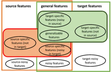
A source model usually includes both generalizable features and source-specific features. A target model will include generalizable features and target-specific features. Therefore, the intersection of source model and target model is the set of generalizable features (Figure 1).
Figure 1 Types of features in the source and the target (Red box: features in the source model. Green box: features in the target model)
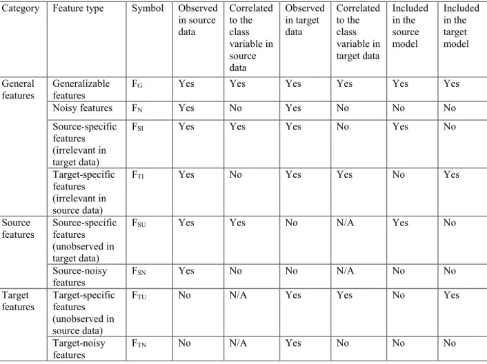
Table 1 summarizes eight different types of features of transfer learning tasks. General features are features of both the source and the target. General features include generalizable features, noisy features, source-specific features that are irrelevant in the target, and target-specific features that are irrelevant in the source. Source features are features that only appear in the source, including source-specific features that are unobserved in the target and source-noisy features. Target features are features that only appear in the target, including target-specific features that are unobserved in the source and target-noisy features.
Table 1 Different types of features in transfer learning tasks
Category Feature type Symbol Observed in source data Correlated to the class variable in source data Observed in target data Correlated to the class variable in target data Included in the source model Included in the target model General
features Generalizable features FG Yes Yes Yes Yes Yes Yes
Noisy features FN Yes No Yes No No No
Source-specific features (irrelevant in target data)
FSI Yes Yes Yes No Yes No
Target-specific features (irrelevant in source data)
FTI Yes No Yes Yes No Yes
Source
features Source-specific features (unobserved in target data)
FSU Yes Yes No N/A Yes No
Source-noisy
features FSN Yes No No N/A No No
Target
features Target-specific features (unobserved in source data)
FTU No N/A Yes Yes No Yes
Target-noisy
When I build the target model, a key step is to identify the generalizable features and the target-specific features. Once I have both source data and target data to identify different feature types, I can use some feature selection approaches to identify influential feature sets for source data and target data respectively. In this dissertation, I mainly used information gain score (Kent 1983) or correlation-based feature selection (Hall 1999).
3.2.1 Information Gain Score
The information gain score is commonly used as an indicator of a finding’s discriminative ability. It is the expected reduction in entropy after using a candidate feature to divide data into subgroups. Entropy is calculated using ∑ −𝑝𝑝𝑖𝑖 𝑖𝑖𝑙𝑙𝑃𝑃𝑙𝑙2𝑝𝑝𝑖𝑖, where 𝑝𝑝𝑖𝑖 is the probability of class i, and it is estimated using the proportion of class i in the training dataset.
As described in Table 1, the intersection of relevant feature sets in the source and the target are generalizable features. The remaining features in the relevant feature set of the target are target-specific features. They are either unobserved or irrelevant in the source. I calculate the information gain score of each candidate feature in the source and the target, respectively. Features with information gain scores greater than a threshold are included.
3.2.2 Correlation-based Feature Selection
Another feature selection approach is correlation-based feature selection (CFS). This approach has a central criterion that good feature sets contain features that are highly correlated with the class, yet uncorrelated with each other. The CFS approach has been found to be able to quickly identify noisy features and influential features as long as their relevancies do not strongly depend on other features (Hall 1999).
Similar to the information gain score approach, the CFS approach can be used to select a relevant feature set of the source and the target, respectively. Then, the intersection of the two sets is the set of generalizable features. The remaining features in the relevant feature set of the target is the set of target-specific features.
3.3BTLSD Algorithm
The BTLSD algorithm aims to combine source data and target data for the classification task in the target. After obtaining data from the source, the simplest way is to mix source and target data and use the shared features of them (general features in Figure 1) for model development. However, this approach is not able to include target-specific features into final models.
The BTLSD algorithm is particularly designed to be able to remove source-specific features (noisy in target) and inject target-specific features into the model. The algorithm first identifies the generalizable features and target-specific features. Some target-specific features may be unobserved (FTU in Table 1), or irrelevant (FTI in Table 1) in the source data. Their counts are
(Naïve Bayes and K2) to build Bayesian network models with the selected features (i.e., generalizable features and target-specific features) using both target data and source data. The pseudocodes are provided in Appendix A.
Because transfer learning tasks usually have a large source training sample and a relatively small target training sample, it is possible that the source data will dominate the target data for model development. This can be harmful especially when the source and the target distributions are very different. Therefor