Cap-and-Trade Programs Under Delayed Compliance
Makoto Hasegawa
yStephen Salant
zApril 19, 2012
Abstract
Although sometimes exceedingly complex, cap-and-trade regulations share some common features which have escaped notice. Previous analyses have assumed that …rms must be in continual compliance, surrendering permits as they pollute. As we showed in a companion paper (Hasegawa and Salant, 2010), if …rms must cover their emissions on a continuing basis, then in the absence of uncertainty, the price path of permits may remain constant over measurable intervals while the government sells additional permits at a ceiling price or may even collapse in response to an anticipated injection of permits through a government auction.
Despite the implicit assumption of this literature, however, no cap-and-trade pro-gram actually requires continual compliance. The three federal bills and California’s AB-32, for example, all permit …rms to be out of compliance for substantial intervals (one year in some cases and as long as three years in other cases). Such “delayed compliance” programs require that …rms surrender permitsperiodically to cover their cumulative emissions since the last compliance period. Anticipated injections of ad-ditional permits during the compliance period should not a¤ect the rate of change of price under delayed compliance although they will a¤ect the position of the equilibrium price path. We develop a general methodology for analyzing the e¤ects of such injec-tions of additional permits. Using it, we explain why the sales provisions of one federal bill (Kerry-Lieberman) might generate a speculative attack in the permit market and why one provision of the California program may undermine the very existence of an equilibrium.
We would like to thank Andrew Stocking for alerting us to the delayed compliance provision and Har-rison Fell for helpful discussions. Hasegawa acknowledges the …nancial support provided by the Nakajima Foundation and the Yamada Academic Research Fund. Salant presented an earlier draft of this work at the Community Colloquium and at the 13th Occasional California Workshop on Environmental and Resource Economics at UCSB, when he was in residence at the Bren School as a UCE3 Senior Fellow.
yDepartment of Economics, University of Michigan. E-mail: [email protected].
zDepartment of Economics, University of Michigan and Resources for the Future. E-mail:
1
Introduction
Cap-and-trade programs are being utilized as the main vehicle to combat global warming by national and state governments of advanced countries. Such regulations are sometimes exceedingly complex. Nonetheless they share some common features. First, although …rms subject to the regulations are required to surrender permits to cover their carbon emissions, they are not required to surrender permits on a continuing basis (“continual compliance”) but only periodically. As a result, a …rm may emit carbon without possessing the permits to cover its emissions as long as it acquires su¢ cient permits by the compliance date. We refer to this aspect of the regulations as “delayed compliance.” In the case of the California law (AB-32), for example, the compliance period is initially two years and subsequently three years (although a fraction of the permits must be surrendered earlier as a down-payment). In the case of the three federal bills that failed to become law, the compliance period was one year.1 Second, while some permits are issued at the outset of a compliance period,
provision is made for the government to inject additional permits into the market later in the compliance period. Third, while permits may be stored (“banked” ) over time for later use, these programs prohibit or severely restrict the opportunity to borrow from future allocations.
These common features have consequences that have escaped notice. Previous analyses have assumed that …rms must be in continual compliance. Under this assumption, a sizable literature has developed to assess the welfare bene…ts of holding back some of the permits that could have been allocated at the outset and using them subsequently to hold down the price through auctions or sales at …xed prices. Such policies are classi…ed as “price collars”or “safety valves.”2Burtraw et al. (2010) …nd that a price collar (also called a “symmetric safety
valve” in the paper) outperforms a safety valve in a static setting. Fell and Morgenstern (2010) and Fell et al. (2010) simulate a dynamic stochastic model of a cap-and-trade program with a price collar or a safety valve.3 Fell and Morgenstern (2010) …nd that price collar mechanisms are more cost-e¤ective than both purely quantity-based mechanisms and safety valve mechanisms for a given level of expected cumulative emissions. They also …nd that the combination of a price collar with banking and borrowing systems can achieve expected cost as low as a tax with lower emissions variance. Fell et al. (forthcoming) …nd that hard
1Waxman-Markey’s “American Clean Energy and Security Act of 2009,”, Kerry-Boxer’s “Clean Energy
Jobs and American Power Act of 2009,” and Kerry-Lieberman’s “American Power Act of 2010.”
2For a valuable explanation of the origins of the safety valve concept and its evolution in the climate
context, see Jacoby and Ellerman (2004).
3In a dynamic context, intertemporal trading of emissions permits matters for economic e¢ ciency.
Cron-shaw and Kruse (1996) and Rubin (1996) show that emissions trading allowing banking and borrowing of emission permits achieves the least-cost outcome.
collars, which ensure unlimited supply of reserve allowances to defend a ceiling price yield lower net present value of expected abatement costs than soft collars, price collars with limited supply of reserve allowances, for the same level of the expected cumulative emissions net of o¤sets. Most recently, Hasegawa and Salant (2010) have shown that if …rms must cover their emissions on a continuing basis, then in the competitive equilibrium, the price path of permits may remain constant over periods while the government is selling additional permits at a ceiling price or may even collapse in response to a government auction. Clearly, no rational private agent would hold permits in the face of such capital losses. But the government sales of additional permits would enable …rms to acquire the necessary permits to remain continually in compliance.4
Despite this sizable literature analyzing the e¤ects of permit auctions and sales under a regime of continual compliance, such policies remain to be investigated under the actual regime of delayed compliance.5 With delayed compliance, …rms purchase the permits they
will ultimately need only at those instants within the compliance period when the permit price has the lowest capitalized value at the compliance date.
In the absence of uncertainty, prices can never rise faster than the rate of interest under either compliance regime; otherwise traders would attempt to buy low and sell high on an in…nite scale. In contrast to the case of continual compliance, however, under delayed compliance prices can also never rise slower than the rate of interest. For suppose the contrary. Then the highest capitalized price would strictly exceed the lowest capitalized price. But then everyone with an initial allocation of permits would want to sell them at the highest capitalized price and there would be no one on the other side of the market willing to buy permits at that price; as a result, there would be massive excess supply. It follows that in any equilibrium under delayed compliance, prices must rise throughout the compliance period at the rate of interest. Anticipated government auctions or sales from a …nite reserve at a …xed price will not slow this rate of price appreciation although, as we will show, they will determine the position of the price path or, equivalently, the permit price prevailing at the compliance date.
The equilibrium permit price at the compliance date equates the demand for permits
4If unlimited “borrowing” were permitted, such price drops would not occur since permits could be
borrowed from a future low-price period and sold earlier at a higher price. But every proposal severely restricts such borrowing.
5There are three exceptions: Murry et al. (2009) and Wood and Jotzo (2011) were the …rst to note that
a price collar implemented by reserve auctions would not provide a ceiling or a ‡oor on emission permits depending on the demand for permits at the time of the auctions and the amount of initially grandfathered permits; however they do no formal modelling. Holland and Moore (2011) identify circumstances su¢ cient for equilibria under the two regimes to coincide, which as we shall see excludes from consideration most of the auctions and sales imbedded in these programs.
required to cover the cumulative emissions which have occurred since the last compliance date with the cumulative supply of permits provided by the government over that period.6
The following algorithm can then be used to determine the permit price at the compliance date.
For each possible terminal price, determine the (unique) associated price path over the compliance period. To determine the cumulative demand for permits along that path, note that at every instant …rms will abate up to the point where their marginal cost of abatement capitalized to the compliance date equals the permit price anticipated to prevail at that date. Compute the aggregate cumulative emissions of the regulated entities over time. Firms will need a matching number of permits at the compliance date. This procedure provides one price-quantity pair on the cumulative demand curve for permits. Repeat the procedure to generate the other points on the demand curve.
Deriving the cumulative supply of permits as a function of the terminal price is somewhat trickier. Since all prices on each associated price path will have the same capitalized value, private agents will not care when they sell as long as they hold zero permits after the compliance period ends. Hence cumulative supply of permits over the period will consist of the initial allocationsplus the subsequent injections of additional permits. These injections depend on the …ne details of particular regulations as we will illustrate using provisions from California’s cap-and-trade program AB-32 which begins later this year and from the three Congressional bills which died in Congress. All four programs envision an initial allocation of permits supplemented by subsequent injections of additional permits during the compliance period. The programs di¤er, however, in the rules governing these injections. For example, while all these programs prescribe a periodic sequence of auctions with pre-announced reserve prices, the programs di¤er in whether permits unsold in one auction can be re-o¤ered in subsequent auctions. As we show, California AB-32 has a troublesome provision for o¤ering unsold permits in subsequent auctions that induces a jump in the supply of permits; under this rule, there may be no price path that will clear the permit market.
In addition to auctions, the programs envision sales at pre-determined prices; but here too the terms of these sales di¤er. The California plan contemplates sales of speci…ed amounts at speci…ed prices from an “Allowance Price Containment Reserve”shortly after each quarterly auction whereas the Kerry-Lieberman (2010) bill proposed sales of permits at a …xed price over a designated time interval or until the “Cost Containment Reserve” was depleted.
In the next section, we discuss the determination of cumulative demand for permits as a
6As an analytical simpli…cation, we assume that it is illegal or unpro…table to carry permits from one
compliance period to the next. The following algorithm can then be used to determine the permit price at the compliance date. However, the algorithm in the text is easily modi…ed if carryovers between compliance periods is permitted.
function of the last price on a price path rising at the rate of interest. We then discuss the cumulative supply of permits as a function of the last price on that path. We show how the supply curve depends on the particular provisions of the emissions trading program. The last price on the equilibrium price path is determined by the intersection of the cumulative demand and supply curves. We will also note when the equilibrium price path under continual compliance di¤ers from the path under delayed compliance. Such di¤erences occur when …rms would not receive injections of permits soon enough to surrender them under continual compliance. In such cases, excess demand occurs and permit prices must initially be higher (and emissions per unit time initially lower) under continual compliance.
2
Preliminaries
Under delayed compliance, …rms will purchase permits at the lowest price, capitalized to the date of compliance. Since, as explained previously, the equilibrium price path under delayed compliance must rise at the rate of interest, every price is lowest and we may index such paths by the price expected to prevail at the date of compliance. Denote that price as P:
We assume that …rm i (i2 f1; : : : ; ng) can reduce its emissions to rate ei(t) by abating
at cost ci(ei(t)); where …rm i’s cost is a strictly decreasing, strictly convex, di¤erentiable
function of emissions. To avoid corners, we assume the Inada condition holds: c0
i(e)! 1
as e ! 0: Moreover, at a su¢ ciently high level of emissions (“baseline emissions,”ei), the
…rm’s cost declines to zero and approaches that level at a zero slope: ci(ei) = c0i(ei) = 0:
Then …rmi chooses its emissions pathei(t) to minimize its total cost of complying with the
cap-and-trade regulation. It minimizes ci(ei(t))er(T t)+ei(t)P: Its optimal emissions path
therefore solves:
c0i(ei(t)) =Per(t T); for t2[0; T] and i= 1; : : : n: (1)
Given the properties of then cost functions, the emissions of each …rm at any instant are a continuous, strictly decreasing function of P. From the emissions paths of the …rms, we can determine the cumulative aggregate demand for permits through time as a function of
P: D(P; ) = Z t=0 n X i ei(t)dt for 2[0; T]: (2)
D(P; ) is continuous, strictly decreasing in its …rst argument and strictly increasing and strictly concave in its second argument. The intercepts are D(P;0) = 0 and D(0; ) =
Pn
For any particular government method of injecting permits, we can de…ne S(P; ) as the government’s cumulative supply of permits until time on a price path rising at the rate of interest and ending at P. Under delayed compliance, any price path such that
D(P; T) = S(P; T)equilibrates the market.
To determine when the equilibrium price path under delayed compliances generates a disequilibrium under continual compliance, we will have to compute the cumulative supply and demand for permits at any time under continual compliance when the price rises throughout at the rate of interest, reaching P at T: A given method of injecting permits will generate the same cumulative supply S(P; ) under the two regimes. Moreover, under continual compliance …rmi’s demand for permits at is also given by equations (1) and (2). Provided the price path rises at the rate of interest, each …rm’s cumulative demand from the outset to timeT will be the same under the two regimes.7
However, equilibrium under continual compliance requires thatD(P; ) S(P; )forall 2 [0; T) in addition to D(P; T) = S(P; T). That is, in the continual compliance regime, agents must be provided enough permits to be able to cover their emissions at every instant and not merely the last one. Since the requirement of equilibrium is more restrictive under continual compliance, price paths that equilibrate the market under delayed compliance fail to equilibrate it under continual compliance.
3
Auctions with Reserve Prices
Throughout we will assume that g permits are “grandfathered” at the outset and that the number grandfathered is smaller than the cumulative emissions that would have occurred without a cap-and-trade program (g < T Pni=1ei).
In this section, we assume that the government commits at the outset to conduct a sequence of auctions. The date, amount, and reserve price of each auction is announced at the outset. Let ti denote the date of theith auction, ai its amount, and pi its reserve price
(assumed strictly positive) for i = 1; : : : A, where A is the total number of auctions to be held during the compliance period, [0; T].
To determine the equilibrium price path under delayed compliance, we construct the cumulative demand and cumulative supply curves and determine their unique point of
inter-7The cumulative demands no longer coincide on price paths that rise somewhere more slowly than the
rate of interest. Suppose, for example, that the price is constant atPuntilT. Then at every instant under continual compliance emissions would solve c0
i(ei(t)) = P; fort 2 [0; T]andi = 1; : : : nwhich is strictly smaller than the solution to (1); hence, cumulative demand untilT would be strictly smaller on such a price path under continual compliance. However, this observation is unimportant since the equilibrium price path under delayed compliance must always rise at the rate of interest and we will be checking whether such a price path equilibrates the permit market under continual compliance.
section. The cumulative demand curve is simply D(P; T), which is downward-sloping with respect to P. The cumulative supply curve S(P; T) is a step-function. For the price path with the terminal price of zero, aggregate supply consists of the g grandfathered permits. As the terminal price is increased, it eventually equals lowest capitalized reserve price. At that terminal price, the cumulative supply is indeterminate— as small as g and as large as
g plus the amount o¤ered at the auction with the lowest capitalized reserve price. If the terminal price is slightly higher, the cumulative supply equals the upper end of this interval. Cumulative supply would remain at that level until the terminal price reached the next-to-the-lowest capitalized reserve price. A su¢ ciently high terminal price will equal the highest of the capitalized reserve prices of the A auctions. Any higher terminal price will elicit the maximal supply of g+PAi=1ai permits.
There exists a unique equilibrium price path and terminal price,P:Existence follows since a zero terminal price would generate excess cumulative demand (by assumption,T Pni=1ei >
g) while a su¢ ciently high terminal price would generate excess cumulative supply (cumula-tive supply g+PAi=1ai is bounded away from zero and cumulative demand approaches zero
for su¢ ciently highP). Moreover the intersection point must be unique since, at any higher price, demand is strictly smaller and supply weakly larger while, at any lower price, demand is strictly larger and supply weakly smaller.
To construct the supply curve geometrically, proceed as follows: (1) on a diagram with time on the horizontal axis and price per permit on the vertical axis (see Figure 1), record the date and reserve-price pair (ti;pi) of each of theAauctions; (2) determine the capitalized
value (Pi) of each reserve price by drawing through each of theseApoints a price path rising at the rate of interest and noting its height atT (Pi =pier(T ti)). For terminal prices smaller
than the smallest capitalized reserve price, only theg grandfathered permits are supplied to the market. For higher prices, the cumulative supply functionS(P; T)will have a horizontal step of length ai at height Pi for i= 1; : : : A:
Whenever the exogenous reserve prices rise by less (respectively, more) than the rate of interest, Pi > Pi+1 (respectively, Pi < Pi+1). Whenever the exogenous reserve prices rise by exactly the rate of interest, every reserve price has the same capitalized value at the compliance date.
In Figure 1, all auctions have the same reserve price (pi =pj). Since these reserve prices rise by less than the rate of interest, P1 > P2 > P3 > P4. In the example portrayed, the equilibrium terminal price P* is contained in the open interval (P4;P3): Hence, no bids are accepted at the …rst three auctions but a4 is sold at the fourth auction. Therefore, in equilibrium emissions equal g+a4:
equilibrium price path Permit Price 1
P
2P
3P
4P
p
1t
t
2t
3t
4T
0
Cumulative EmissionsTerminal Permit Price
S
(
P
,
T
)
g
4a
3a
2a
1a
)
,
P
(
T
D
)
P
,
(
g
+
a
4 * TimeFigure 1: The Cumulative Demand and Supply, and the Equilibrium Price Path in the Case of Reserve Price Auctions
to the number grandfathered, then the cumulative supply curve would become g +a4 for terminal prices belowP4 but the modi…ed cumulative supply curve would still intersect the unchanged cumulative demand curve at the same point. Hence, the equilibrium price path would not change under delayed compliance nor would the cumulative emissions it induces. Alternatively, if the government had grandfathered no permits but had instead auctioned these g permits along with thea4 permits at t4, then the cumulative supply at prices below P4 would be zero and the cumulative supply atP4 would be as large asg+a4: Nonetheless this modi…ed cumulative supply curve would still intersect the cumulative demand curve at the same point. Neither change would a¤ect the equilibrium under delayed compliance.
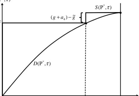
If the entire sum of permits was grandfathered at the outset, then this same price path would also equilibrate the market under continual compliance. But if all of these permits were made available instead at t4, then a disequilibrium would inevitably occur since, for some < T; D(P; ) > S(P; ): In Figure 2, we plot cumulative supply and demand until along the equilibrium price path under delayed compliance (the price path ending atP ):
Since the path generates an equilibrium under delayed compliance, the two curves intersect at T: An equilibrium under continual compliance requires in addition that the cumulative supply curve lies nowhere strictly below the cumulative demand curve for 2[0; T):We have drawn the boundary case where ~g =D(P ; t4) permits are grandfathered and (g +a4) g~
g ~ g a g ~ ) ( + 4 − ) , P ( * τ D ) , P ( * τ S τ T 4 t ) , P ( * τ S ) , P ( * τ D 0
Figure 2: The Boundary Case in the Case of Reserve Price Auctions
are auctioned att4. If the government grandfathered strictly less than ~g permits and added them instead to the amount auctioned att4, then the equilibrium under delayed compliance could no longer be supported as an equilibrium under continual compliance. Instead, the price path would consist of segments rising at the rate of interest, separated by a downward jump at t4.
Returning to the case of delayed compliance, suppose that cumulative demand was so large thatP 2(P2;P1):That is, every auction aftert1sells out, but bids in this …rst auction are below its reserve price (p1): Under the rules of California’s AB-32, thea1 permits which failed to sell in the …rst auction would be returned to the “Auction Holding Account.” Some of these permits would be available for sale in the fourth auction since it would have occurred “after two consecutive auctions have resulted in an auction settlement price greater than the applicable Auction Reserve Price.” However, not all of the a1 permits could be made available. At most the number of permits which can be added to the auction at t4 is 25% ofa4:It is not clear to us how many of these permits would be o¤ered and who decides, but at the old equilibrium price excess supply would occur because these unsold additional permits would be o¤ered in an auction where the market price exceeds the reserve price. As a result, the equilibrium price path under delayed compliance would rise to a lower terminal price.
O¤ering unsold permits for sale if and only if permits are sold at two subsequent auctions in a row can create a situation where no competitive equilibrium exists. Suppose, for example, that no bids exceed the reserve price in the …rst auction but the next two auctions sell out. Suppose cumulative demand is su¢ ciently high that in the absence of the rule regarding unsold permits that P 2(P2;P1). Under this rulemin(a1;0:25a4) of the permits from the …rst auction can be o¤ered in the fourth auction. If min(a1;0:25a4) > D(P2) g a2 a3 a4 = D(P2) D(P ) then there will be excess supply at any terminal price equal to or exceeding P2.8 But at any terminal price strictly belowP2, there will be excess demand since, in the absence of two consecutive auctions where permits sold, none of the unsold permits from auction 1 can be o¤ered for sale in auction 4, and then D(P) > g+a3+a4 holds for all P<P2.
4
Sales at Speci…ed Prices
Permits can also be injected during the compliance period by sales at a speci…ed price, which we denotep:To simplify, we assume in this section that all permits not grandfathered at the outset are injected by such sales. Such sales can occur over a speci…ed time interval which commences at tc and …nishes at tf or until all of the R permits in the “Cost Containment
Reserve”have been sold. The Kerry-Lieberman bill envisioned such sales over a …nite inter-val. They resemble a continuum of auctions with reserve price p over the time interval[tc; tf]
but withRavailable in the initial auction, andeverything unsold in one auction immediately available for sale in subsequent auctions.
Since the sales price over the interval is constant, the price at tf has the smallest
capital-ized value (Pf =per(T tf)). In Figure 3, we depict the interval of o¤ers and the sales price. As in Figure 1, we depict Pf by noting the terminal price on the path through the point (tf; p) rising at the rate of interest. To derive the cumulative supply curve, note that if the
terminal price is strictly smaller than Pf; then nothing would sell during this time interval and the cumulative supply would just be g. If the terminal price is strictly larger, then the cumulative supply would be g+R: If the terminal price is exactly Pf then the cumulative supply is any number of permits in the closed interval [g; g+R]:
Suppose cumulative demand is su¢ ciently large that under delayed compliance the ter-minal price strictly exceedsPf. ThenR permits sell instantaneously, either at some interior date 2 (tc; tf) or at the …rst moment of the sale (tc). In either case, such purchases at
an in…nite rate are just like “…rst-generation” speculative attacks which have been widely
8We use the excess supply condition atP
2: D(P2)< g+ min(a1;0:25a4) +a2+a3+a4and the de…nition ofP : D(P ) =g+a2+a3+a4.
equilibrium price path Permit Price c
P
fP
p
ct
t
fT
0
Cumulative EmissionsTerminal Permit Price
S
(
P
,
T
)
g
R
)
,
P
(
T
D
)
P
,
(
g
+
R
* *τ
TimeFigure 3: The Cumulative Demand and Supply, and the Equilibrium Price Path in the Case of Sales at Speci…ed Prices
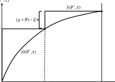
discussed in the literatures on foreign exchange markets and on commodity agreements.9 Suppose in the equilibrium under delayed compliance that the terminal price is P and cumulative emissions are g+R: Suppose the speculative attack occurs at the interior point
> tc. Reallocating theg+R permits between the initial allocation and the Cost
Contain-ment Reserve will not alter the equilibrium price path or the date of the attack under delayed compliance. Such reallocation may however a¤ect the price path under continual compli-ance. In Figure 4, we depict the boundary case where the initial allocation g = D(P ; ) andg+R =D(P ; T), implying thatR=D(P ; T) D(P ; ). If more permits are moved from the initial allocation to the Cost Containment Reserve, the equilibrium under contin-ual compliance will di¤er from the equilibrium under delayed compliance. In that case, the equilibrium price path under continual compliance will have a segment rising at the rate of interest until tc and then (weakly) dropping to p for an endogenous interval of time before
rising continuously frompagain at the rate of interest. A speculative attack must occur here too but it occurs later than under delayed compliance.
9For a discussion of speculative attacks on commodity ceilings defended by bu¤erstock sales, see Salant
and Henderson (1978) and Salant (1983). For discussions of how their idea was developed further in the international …nance literature, see Krugman (1999) and Flood et al. (2012).
g ~ g R g ) ~ ( + − ) , P ( * τ D ) , P ( * τ S τ T * τ ) , P ( * τ S ) , P ( * τ D 0
Figure 4: The Boundary Case in the Case of Sales at Speci…ed Prices
5
Conclusion
Cap-and-trade programs rather than emissions taxes are being utilized as the main vehicle to combat global warming by national (and state) governments of advanced countries. In the United States, some permits are withheld from the initial allocation and injected sub-sequently into the market by auctions or sales at …xed prices in an attempt to limit price increases (through so-called “price collars”or “safety valves”). The e¤ect of these subsequent injections depends on whether the program requires regulated …rms to be in compliance con-tinually or merely periodically. Until now, virtually all analyses have assumed continual compliance even though actual programs always require delayed compliance.
The purpose of our paper has been to develop a methodology for analyzing the e¤ects of such injections in a regime of delayed compliance. In the process of illustrating the use of this methodology, we identi…ed two consequences of the provisions of cap-and-trade programs (potential speculative attacks and nonexistence of equilibrium) that have escaped notice.
We have also clari…ed when the equilibrium under continual compliance di¤ers from the equilibrium under delayed compliance. We have not described in detail the e¤ects of such injections under continual compliance since no actual programs require that.10
10Interested readers are referred to our companion paper (Hasegawa and Salant (2010) where such a
We have assumed away all forms of uncertainty in the current analysis but will address this issue in the future. Permit markets may be subject to three kinds of uncertainty: (1) ongoing regulatory uncertainty that, when resolved, will result in a nonstochastic environment; (2) uncertainty about the aggregate demand for permits that will be resolved at a …xed date in the future by an information disclosure; and (3) aggregate demand shocks each period. McWilliams and Moore (2011) have shown the importance of regulatory uncertainty in the SO2 permit market. The consequences of disclosing information at a known time about the demand for permits is illustrated by the collapse of the permit price in Europe following the disclosure of low demand for permits. In the case of demand shocks each period, the price path would become stochastic rather than deterministic. But it appears that little would change under uncertainty if agents are risk neutral. In no equilibrium will the current price be strictly smaller than the price expected at any date in the future discounted back to the current period; otherwise, risk-neutral speculators would purchase for subsequent re-sale on an in…nite scale. If the current price is strictly higher than every price expected in the future, properly discounted, then holders of the initial allocation will want to sell their permits in the current period but no buyers would want to buy them. Since there can be no competitive equilibrium in either situation, It follows that, if any equilibrium exists, the price in any period must be equal to the price then expected in every future period, discounted back appropriately. Moreover, in the …nal period of the compliance period, all permits would be surrendered to the government and, if agents had insu¢ cient permits to cover their cumulative emissions, they would have to pay a well-speci…ed penalty.
References
[1] Burtraw, Dallas, Karen Palmer, and Danny Kahn. 2010. “A Symmetric Safety Valve.”
Energy Policy 38(9), pp. 4921-4932.
[2] Cronshaw, Mark B. and Jamie B. Kruse. 1996. “Regulated Firms in Pollution Permit Markets with Banking.”Journal of Regulatory Economics 9(2), pp. 179-189.
[3] Fell, Harrison, Dallas Burtraw, Richard D. Morgenstern, and Karen L. Palmer. Forth-coming. “Soft and Hard Price Collars in a Cap-and-Trade System: A Comparative Analysis.”Journal of Environmental Economics and Management.
[4] Fell, Harrison and Richard D. Morgenstern. 2010. “Alternative Approaches to Cost Containment in a Cap-and-Trade System.”Environmental and Resource Economics
47(2), pp. 275-297.
Thinking about Currency Crises,” In Lucio Sarno, Jessica James, and Ian Marsh (eds.), Handbook of Exchange Rates, John Wiley & Sons, Inc., Chapter 25.
[6] Hasegawa, Makoto and Stephen Salant. 2010. “The Proposed Cap-and-Trade Program under Continual Compliance: The Case of the Unbuttoned Collar.”Working Paper, University of Michigan.
[7] Holland, Stephen P. and Michael R. Moore. 2011. “Market Design in Cap and Trade Programs: Permit Validity and Compliance Timing.” mimeo.
[8] Jacoby, Henry D. and A. Denny Ellerman. 2004. “The Safety Valve and Climate Policy.”
Energy Policy 32(4), pp. 481-491.
[9] Krugman, Paul. 1999. “Currency Crises,” available at:
http://web.mit.edu/krugman/www/crises.html.
[10] McWilliams, Michael and Michael R. Moore. 2011. (Conference Presentation)
[11] Murray, Brian C., Richard G. Newell, and William A. Pizer. 2009. “Balancing Cost and Emissions Certainty: An Allowance Reserve for Cap-and-Trade.”Review of Environmental Economics and Policy 3(1), pp. 84-103.
[12] Rubin, Jonathan D. 1996. “A Model of Intertemporal Emission Trading, Banking, and Borrowing.”Journal of Environmental Economics and Management 31(3), pp. 269-286.
[13] Salant, Stephen W. 1983. “The Vulnerability of Price Stabilization Schemes to Specu-lative.”Journal of Political Economy 91(1), pp. 1-38.
[14] Salant, Stephen W. and Dale Henderson. 1978. “Market Anticipations of Government Policies and the Price of Gold.”Journal of Political Economy 86(4), pp. 627-648. [15] Wood, Peter J. and Frank Jotzo. 2011. “Price Floors for Emissions Trading.”Energy