Dynamic Particle Swarm Optimization to Solve Multi-objective Optimization Problem

Procedia Technology 6 ( 2012 ) 283 – 290

2212-0173 © 2012 The Authors. Published by Elsevier Ltd. Selection and/or peer-review under responsibility of the Department of Computer Science & Engineering, National Institute of Technology Rourkela

doi: 10.1016/j.protcy.2012.10.034

2nd International Conference on Communication, Computing & Security [ICCCS-2012]

Dynamic Particle Swarm Optimization to Solve

Multi-objective Optimization Problem

a_{Department Of Computer Science And Engineering, RTMNU University, RCERT, Chandrapur (M.S), 442401, India} b_{Department Of Computer Science And Engineering, RTMNU University ,RCERT, Chandrapur (M.S),442401,India}

Abstract

Multi-objective optimization problem is reaching better understanding of the properties and techniques of evolutionary algorithms. This paper presents the Dynamic Particle Swarm Optimization algorithm for solving multiobjective

PSO in terms of swarm size, topology and search space. In this paper swarm size criteria for dynamic PSO is considered. Experiment conducted for standard benchmark functions of multi-objective optimization problem, which shows the better performance rather the basic PSO.

© 2012 Published by Elsevier Ltd.

Selection and/or peer-review under responsibility of the Department of Computer Science & Engineering, National Institute of Technology Rourkela

Keywords- Optimization, Particle swarm optimization, Dynamic PSO, Multiobjective Optimization

______________________________________________________________________________________________________________ 1. Introduction

Numerous works related to subpopulation manipulation in multiobjective evolutionary algorithms (MOEAs) have consistently shown that the implementation of the subpopulation concept coupled with other techniques yields more efficient and effective designs, particularly in enhancing the population diversity. In recent years, the subpopulation concept is incorporated into particle swarm optimization (PSO), generically referred to as swarm PSO. In fact, multiple-swarm PSO bears a remarkable resemblance with the mixed-species flocking. The particle multiple-swarm optimizer (PSO) is a relatively new technique. Particle swarm optimizer (PSO), introduced by Kennedy and Eberhart in 1995[1], emulates flocking behaviour of birds to solve the optimization problems. In PSO, each solution is regarded as a particle. All particles have fitness values and velocities. During an iteration of the PSO, each particle accelerates independently in the direction of its own personal best solution found so far, as well as the direction of the global best solution discovered so far by any other particle. Therefore, if a particle finds a promising new solution, all other particles will move closer to it, exploring the

© 2012 The Authors. Published by Elsevier Ltd. Selection and/or peer-review under responsibility of the Department of Computer Science & Engineering, National Institute of Technology Rourkela Open access under CC BY-NC-ND license.

solution space more thoroughly. Typical implementations of PSO start with a reasonably sized swarm (about 40 particles). These particles are initialized with a random distribution within the solution space. As the iterations proceed, the particles will tend to cluster towards a global optimum. In each iteration, the fitness function is evaluated to find the optimality of each proposed solution (particle), and then the location of each particle is updated to drive towards convergence. Typically, the optimization process is repeated about minimum 10,000 times to allow the particles to converge on the global optimum. If the fitness function is complex, then the per-iteration evaluation and update process will tend to be long. After a while, the particles tend to converge and repeating the evaluation for all particles per iteration will not add substantial improvement. Most particles would have converged on extremely close locations that there is no need to repeat the evaluation and update for each and every one of them.

In this paper we have conducted the experimental performance on some multi-objective

with the dynamic PSO. The simple PSO is considered as fixed swarm size and fixed topological environment. We perform this simulation work with different swarm size in each iteration of PSO and also having variation in topology. The remainder of this paper is organized as follows: section 2 present a brief review on PSO , section 3 describe some relevant works of multiobjective optimization, section 4 describe detail of the Dynamic PSO algorithm is elaborated. Comprehensive study and Experimental results are discussed in section 5, and finally, section 6 provides concluding remarks of study.

2. Literature Survey

PSO was originally proposed by Kennedy and Eberhart [1] for optimization. The optimization technique was inspired by bird flocking and animal social behaviours. In PSO, the particles operate collectively like a swarm that flies through the hyper dimensional space to search for possible optimal solutions. The behaviour of the particles is influenced by their tendency to learn from their personal past experience and from the success of their peers to adjust the flying speed and direction. Research in fusing the multipleswarm concept into PSO is well established in solving SOPs and multimodal problems [2]. Swarm Intelligence (SI) is an innovative distributed intelligent paradigm for solving optimization problems that originally took its inspiration from the biological examples by swarming, flocking and herding phenomena in vertebrates. Ant colony optimization, Genetic algorithm, particle swarm optimization are various evolutionary algorithms proposed by researchers. Due to simplicity in PSO equation and fast convergence, PSO is found to be best among these. After analysing each parameter in PSO equation

inertia weight in the basic equation. It can be imagined that the search process for PSO without the first part is a process where the search space statistically shrinks through the generations. It resembles a local search algorithm. Addition of this new parameter causes exploration and exploitation in search space. Firstly value of w was kept static. Later on it was kept linear from 0.9 to 0.4. Eberhart Russell and Shi Yuhui [4] in 2000 compare these results with constriction factor. A small

constriction method is used,

to 0.729. According to Clerc, addition of constriction factor may be necessary to insure convergence of particle swarm optimization algorithm The PSO algorithm with the constriction factor can be considered as a special case of the algorithm with inertia weight.

F. van den Bergh, A. P.E ngelbrecht invented Guaranteed Convergence Particle Swarm Optimizer (GCPSO) [5]. The GCPSO has strong local convergence properties than original PSO. This algorithm performs much better with the small number of particle. The new phenomenon is defined called as

position coincides with the global best position particle, then the particle will only move away from the point if its previous velocity and w are non-zero. If their previous velocities are very close to zero, then all the particles will stop moving once they catch up with the global best particle, which may lead to premature convergence of the algorithm. In fact, this does not even guarantee that the algorithm has converged on a local minimum it merely means that all the

particles have converged on the best position discovered so far by the swarm.

The original PSO is easily fall into local optima in many optimization problems. The problem of premature convergence is solved by the OPSO. It allows OPSO [6] to continue search for global optima by applying opposition based learning. The OPSO use the concept of Cauchy mutation operator. The OPSO based on opposition- based learning method. The OBL method has been given by Hamid R.Tizhoosh, it is explained as when evaluating a solution x to a given problem, we can

guess the opposite ion can reduce. The opposite solution x can be calculated as

x`= a + b - x

where x. R within [a, b]

Hierarchical PSO [7] is known as hierarchical version of PSO called as H-PSO. In this algorithm the particles are arranged in a dynamic hierarchy. In H-PSO, a particle is influenced by its own so far best position and by the best position of the particle that is directly above it in the hierarchy. In H-PSO, all particles are arranged in a tree that forms the hierarchy so that each node of the tree contains exactly one particle. If a particle at a child node as found a solution that is better than the best so far solution of particle at parent node, then these two particles are exchanged. In this algorithm the topology used as regular tree in which hierarchy is defined in terms of height and branching degree. This hierarchy gives the particles different influence on the rest of the swarm with respect to their fitness. Each particle is neighboured to itself and its parent in the hierarchy. Only the inner nodes on the deepest level might have a smaller number of children so that the maximum difference between the numbers of children of inner nodes on the deepest level is at most one. In order to give the best individuals in the swarm a high influence, particles move up and down the hierarchy

Mendes [1] proposed another efficient approach which deals with stagnation is the fully informed particle swarm optimization algorithm (FIPSO) [8]. FIPSO use best of neighbourhood velocity update strategy. In FIPSO each particle uses the information from all its neighbours to update its velocity. The structure of the population topology has, therefore, a critical impact on the behaviour of the algorithm which in turn affects its performance as an optimizer. It has been argued that this happens because the simultaneous

updating its velocity, provoking a random behaviour of the particle swarm.

New Particle Swarm Optimization(NPSO)[9] is the idea of NPSO came from our personal based experience that an also learns from his or her own and worst positi

NPSO has the better solution result than the originally PSO as more seeds are needed when the search dimension gets larger and other parameters might need to change too. The solutions might get out of local minima with more random numbers generated. Position change limits may be tuned too rather than original PSO. Eberhart proposed a discrete binary version of PSO for binary problems [10]. In their model a particle will decide on "yes" or " no", "true" or "false", "include" or "not to include" etc. also this binary values .In binary PSO, each particle represents its position in binary values which are 0 or 1. r better say mutate) from one to zero or vice versa. In binary PSO the velocity of a particle defined as the probability that a particle might change its state to one. The novel binary PSO [9] solve the difficulties those are occurred in binary PSO. In this algorithm the velocity of a particle is its probability to change its state from its previous state to its complement value, rather than the probability of change to 1.

In the PSO world, there exist global and local PSO versions. Instead of learning from the personal best and the best position achieved so far by th velocity is adjusted according to its personal best and the best performance achieved so far within its neighborhood. Kennedy claimed that PSO with large neighborhood would perform better for simple problems and PSO with small neighbourhoods might perform better on complex problems. Kennedy and Medes discussed the effects of different neighborhood topological structures on the local version PSO. Suganthan applied a combined version of PSO where a local version PSO is run first followed by a global version of PSO at the end. Hu and Eberhart proposed a dynamically adjusted neighborhood when they solve the multi-objective optimization problems using PSO. In their dynamically adjusted neighborhood, for each particle, the m closest particles are selected to be its new neighborhood. Veeramachaneni and his group developed a new version of PSO; Fitness-Distance-Ratio based PSO (FDR-PSO) [11], with near neighbor interactions. When updating each velocity dimension, the FDR_PSO algorithm selects one other particle, nbest, which has higher fitness value and near the particle being updated, in the velocity updating

3. Multi-objective Optimization

3.1 Basic of MOP

A multiobjective optimization problem (MOP) can be formally stated as follows: Minimize F(X) = [f1(X), f2 M(X)] T

Subject to X F (1)

Where X is a decision vector with n decision variables, F(X) is the M- -region. Here, we are interested in solving multi objective

optimization problems; that is, the subset of MOPs involving M > 1 objectives [12]. In multi-objective optimization we wish to determine, from among all X F, the particular X* which yields the optimum value for all the objective functions. However, it is unusual that there is a single solution simultaneously optimizing all the (conflicting) objectives. Instead, we are interested in finding a set of trade-off solutions. The most commonly adopted notion of optimality is the so-called Pareto optimality [13] [19].

Let us first define the Pareto dominance (PD) relation. Given two solutions X, Y F, we say that X Pareto-dominates Y, denoted by X Y, if and only if:

m fm(X) fm(Y) ^

m fm fm(Y) (2)

Otherwise, we say that Y is non dominated with respect to X. Finally, we say that a point X* F is Pareto optimal if there is no X F such that X X*.The set of all X* F satisfying this condition constitutes the Pareto optimal set, whose image in objective space is called the Pareto front or trade-off surface.

3.2 Pareto dominance in multi-objective optimization

Pareto dominance (PD) is known to become ineffective as the number of optimization criteria raises. Figure 1 show how the proportion of non dominated solutions in the population behaves with respect to the number of objectives and as the search progresses. We adopted a well-known scalable test problem, ZDT1 [14], and Dynamic PSO (described later in Section 4.4.1) with a population of 100 individuals. A total of 31 independent executions were performed.

From Figure 1, we can clearly see that the increase in the number of objectives raised the proportion of non dominated individuals in the population. Even in the case of the initial population (at generation zero), which is randomly generated, a high percentage of the individuals are non dominated. After a few generations, the population became completely non

dominated in all cases. Thus, no preferences can be set among individuals for selection purposes, leading the algorithm to perform practically a random search. Recently, alternative ranking approaches have been adopted to cope with this issue [6] [15].

4. Dynamic Particle Swarm Optimization

While searching for food, the birds are either scattered or go together before they locate the place where they can find the food. While the birds are searching for food from one place to another, there is always a bird that can smell the food very well, that is, the bird is perceptible of the place where the food can be found, having the better food resource information. Because they are transmitting the information, especially the good information at any time while searching the food from one place to another, conducted by the good information, the birds will eventually flock to the place where food can be found.As far as particle swam optimization algorithm is concerned, solution swam is compared to the bird

moving from one place to another is equal to the development of the solution swarm, good information is equal to the most optimist solution, and the food resource is equal to the most optimist solution during the whole course.

Particle swarm optimization is a global optimization algorithm for dealing with problems in which a best solution can be represented as a point or surface in an n-dimensional space. Hypothesis are plotted in this space and seeded with an initial velocity, as well as communication channel between the particles. Particles then move through the solution space and are evaluated according to some fitness function after each timestamp. Over time particles are accelerated towards those particles within their grouping which have better fitness values. In dynamic PSO there is variation with swarm size and variation in topology. The dynamic particle swarm optimization concept consists of, at each time step, changing the velocity of (accelerating) each particle toward its pbest and lbest (for lbest version). Acceleration is weighted by random term, with separate random numbers being generated for acceleration towards pbest and lbest locations. After finding the best values, the particle updates its velocity and positions with following equations.

V[id]=v[ id]+c1*r(id)*(pbest[id ]-x[ id])+c2*r*(id)(gbest[id]-x[ id])--- (a) x[ id] = x[ id]+v[ id]---(b)

where,

v[id] is particle velocity x[ id] is the current particle

r(id ) is random number between (0,1) c1 and c2 are learning factors usually c1=c2=2.

Algorithm 4.1:- Algorithm for Dynamic Particle Swarm Optimization (DPSO)

The pseudo code of the procedure is as follows, For each particle

Initialize Function value END

Calculate average fitness value Do

For each particle

If fitness value is less than average Consider the particle

Calculate fitness value.

If the fitness value is better than the best Fitness value (pbest) in history Set current value as the new pbest. END

Choose the particle with the best fitness value of all the particles as the gbest

For each particle

Calculate particle velocity according to equation (a) Update particle position according equation (b) END

5. Experimental Work

Here our aim is to solve multi-objective optimization problem with using Dynamic PSO. Dynamic PSO can be defined as varying characteristics of PSO while experimentation is running. Characteristic include topology, swarm size, search space. If topology or swarm size can be change during process, then it is treated as dynamic particle swarm optimization. So we carry out the simulation work with varying swarm size at each iteration .For experimental status we have considered some standards benchmark function of multi-objective optimization.

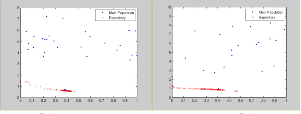
Problems ZDT1, ZDT2 and ZDT3 [14] [21] were adopted for our experimental study. These problems can be scaled to two numbers of objectives and decision variables. We perform simulation to study particle behavior for dynamic PSO to apply for solving multi-objective optimization in 6 dimensional spaces. Values of parameter involved in equation are considered as 0.7 for inertia, 1.49 for c1 and c2 and particle swarm size 100 for first iteration. Simulation has been carried out for 10000 iterations. We first find the dominated point (in figure it has shown by main population) and then we find the cost function value of each dominated point which gives us the set of optimized dominated point.

We find non dominated point ( repository optimized dominated point) and finally we compare this point by using non dominated sorting algorithm which gives us optimized non dominated point. The set of such non dominated point gives us true Pareto front. The result for this problem has shown in following figure.

)LJD)LJE

)LJF

Figure 2. (a), (b) & (c). Superimposed results of dynamic PSO, on benchmark function ZDT1, ZDT2 and ZDT3 with populationsize 100. (a) Showing result for ZDT1 with true Pareto front (convex Pareto- optimal front). (b) Showing result for ZDT2 with truePareto front (non-convex Pareto-optimal front). (c) showing result for ZDT3 with true Pareto front (discreteness feature to the front).{blue point (main population) indicates dominated particle and red point (repository) indicate non dominated particle. The set of nondominated particle gives Pareto front}

6. Conclusion:

The review of Multi-objective PSO algorithm has studied with considering the pre-existing algorithms. Our basic aim of project is to solve multi-objective optimization problem with the help of dynamic PSO. so on the basis of simulation result we conclude that the dynamic PSO gives better optimized value for multi-objective optimization problem

.

References:-

1995.

Multi-[5] 2004.

2007

[7] Stefan Janson & Martin Midden IEEE2005.

[8] [9]

[11] IEEE 2007

in Proceedings of the NAFIPS- Service Center, June 2002, pp. 233 238.

[13] Points are Better

D. Thierens, Ed., vol. 1. London, UK: ACM Press, July 2007, pp. 773 780.

Multiobjective Applications, A. Abraham, L. Jain, and R. Goldberg, Eds. USA: Springer, 2005, pp. 105 145.

- Intelligence, R.

Monroy, C. Reyes, and A. Hernandez, Eds. Guanajuato, M´exico: Springer. Lecture Notes in Artificial Intelligence Vol. 5845, November 2009, pp. 633 645.

[16] 2000

[17] S.- imization for unconstrained

[18] Marco A. Montes de Oca, Thomas Stutzle, Mauro Birattari, Member, IEEE, and Marco Dorigo, Fellow, IEEE, [19] Mario Garza-Fabre, Gregorio Toscano-Pulido, Carlos A. Coello Coello And Eduardo Rodriguez- Effective

Ranking+Speciation=Many-[20] Multiobjective