D S Sharma, R Sangal and E Sherly. Proc. of the 12th Intl. Conference on Natural Language Processing, pages 118–123, Trivandrum, India. December 2015. c2015 NLP Association of India (NLPAI)
Perplexed Bayes Classifier
Cohan Sujay Carlos
Aiaioo Labs Bangalore
India
Abstract
Naive Bayes classifiers estimate posterior probabilities poorly (Zhang, 2004). In this paper, we propose a modification to the Naive Bayes classification algorithm which improves the classifier’s posterior probability estimates without affecting its performance.
Since the modification involves the use of the reciprocal of the perplexity of the class-conditional feature probabilities, we call the resulting classifier the Perplexed Bayesclassifier.
We demonstrate that the modification re-sults in better calibrated posterior proba-bilities on a gender categorization task.
1 Introduction
Probabilistic classifiers work by selecting the most probableclassgiven thefeaturesof the data point being classified, as shown in Equation 1.
arg max
c P(C|F) (1)
Bayesian classifiers transform P(F|C) into
P(C|F)as shown in Equation 2.
P(C|F) = P(F|C)×P(C)
P(F) (2)
Naive Bayes classifiers additionally assume that the featuresf1, f2, f3,etc. are all independent of one another, conditional on the classC, yielding
the following equation.
P(F|C) =Y
i
P(fi|C) (3)
Equation 3 can be substituted into Equation 2 to obtain Equation 4.
P(C|F) =
Q
iP(fi|C)
×P(C)
P(F) (4)
The posterior probability estimates obtained us-ing Equation 4 tend to be extreme as observed in Eyheramendy et al (2003).
Improving the posterior probability estimates of Naive Bayes classifiers might make them more useful for NLP (Nguyen and O’Connor, 1999).
In this paper, we present the Perplexed Bayes
classification algorithm that produces better cali-brated posterior probabilities than the Naive Bayes algorithm and operates with the same accuracy.
2 Related Work
The Naive Bayes classification algorithm is still commonly used as a baseline algorithm for many classification tasks (Rennie et al, 2003), and is re-puted to perform surprisingly well (McCallum and Nigam, 1998; Rennie et al, 2003; Zhang, 2004) though the posterior probabilities might be esti-mated poorly (Eyheramendy et al, 2003; Rennie et al, 2003; Zhang, 2004).
Attempts to improve the Naive Bayes classi-fier have relied on augmentations to relax indepen-dence assumptions (Peng and Schuurmans, 2003; Peng et al, 2004), transformations to correct sys-temic errors (Rennie et al, 2003), the weighting of counts or probabilities (Zaidi et al, 2013; Frank et al, 2003; Webb and Pazzani, 2004) and the subset-ting of features (Langley and Sage, 1994).
0 0.2 0.4 0.6 0.8 1 0
0.1 0.2 0.3 0.4 0.5 0.6 0.7 0.8 0.9 1
Posterior Probability
Observ
ed
Probability
of
Classes
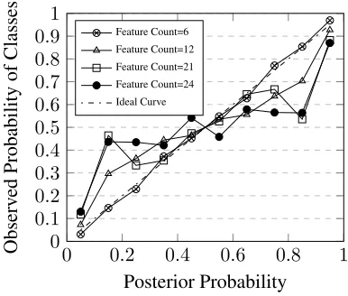
[image:2.612.82.275.41.205.2]Feature Count=6 Feature Count=12 Feature Count=21 Feature Count=24 Ideal Curve
Figure 1: Reliability diagram for a Naive Bayes (NB) classifier.
Our approach is closer to that of Zaidi et al (2013) who used weighted class-conditional fea-ture probabilities. One of the equations that Zaidi suggests could be used (but does not go on to ex-plore) is identical to Equation 8 in this paper.
None of the previous studies has, to our knowl-edge, explored in detail, attempted to generalize, or developed a theoretical foundation for the ap-proach that we describe in this paper.
3 Naive Bayes
In this section, we show that the posterior proba-bilities of the Naive Bayes classification algorithm are not well calibrated.
A Naive Bayes classifier’s posterior probabili-ties were measured on a classification task (iden-tifying the gender of names using the dataset described in Section 5) and a reliability dia-gram (Br¨ocker and Smith, 2007) plotted for differ-ent numbers of features used as shown in Figure 1. A perfectly calibrated classifier’s reliability di-agram would show a straight line (like the ideal curve of Figure 1). As can be seen, the Naive Bayes classifier does not produce well-calibrated posterior probabilities, except for the feature count of6. The calibration is seen to deteriorate as the number of features increases.
In the next section, we propose a modification to the Naive Bayes algorithm to attempt to solve the problem of poor posterior probability estimation.
4 Perplexed Bayes
The perplexityP P(p1, p2, . . . pn)of a set of
prob-abilities{p1,p2, . . . ,pn}is computed as shown in
Equation 5.
P P = 1
(p1×p2×. . .×pn)
1
n
(5)
So, thereciprocal of the perplexityof the prob-abilities is merely theirgeometric meanas shown in Equation 6.
P P–1 = (p1×p2×. . .×pn)
1
n (6)
In the Perplexed Bayes classifier, we combine the class conditional feature probabilities using the geometric mean, as shown in Equation 7.
P(F|C) =
Y
1≤i≤n
P(fi|C)
1
n
(7)
So, the posterior probability equation can be written as shown in Equation 8, where n is the
number of features, andN is the normalizer.
P(C|F) =
Q
iP(fi|C)
1
n ×P(C)
N (8)
We call a classifier that uses the posterior prob-ability equation in Equation 8 the fullyPerplexed Bayesclassifier.
4.1 Assumption
We can show that Equation 8 can be derived from Equation 2 if we assume that the class C is in-dependent of all features but one, and that none of the features is special as shown in Equation 9, where1≤i≤n.
P(C|f1, f2, . . . fn) =P(C|fi) (9)
We can write Equation 9 inndifferent ways, as
follows, because no feature is special.
P(C|f1, f2, . . . fn) =P(C|f1) =P(C|f2) ... =P(C|fn)
(10)
We show below that the assumption embodied in Equation 9 is sufficient for the derivation of Equation 8 (but we have not shown that it is also necessary).
4.2 Derivation
Multiplying together all the terms on both sides of Equation 10 we get Equation 11.
P(C|f1, f2, . . . fn)n=
= Y
1≤i≤n
P(C|fi) (11)
Inverting the terms on the right-hand side of Equation 11 using the Bayesian inversion equation (2), we get Equation 12.
P(C|F)n=
Y
1≤i≤n
P(fi|C)×P(C) P(fi)
(12)
SinceP(C)andP(F)are independent ofi, we
can write Equation 12 as Equation 13.
P(C|F)n=
Y
1≤i≤n
P(fi|C)
× P(C)
n Q
1≤i≤nP(fi)
(13)
P(C|F) =
Y
1≤i≤n
P(fi|C)
1
n
× P(C)
N (14)
Finally, taking thenth root on both sides, we get
Equation 14 (whereN is the normalizer) and this
is substantially the same as Equation 8.
So we have shown that the assumption thatthe class C is independent of all features but one, and that none of the features is special (written as Equation 10) can give us Equation 8.
It is interesting to note that Equation 15, rep-resenting the posterior probabilities of a classifier that uses thearithmetic mean instead of the geo-metric mean, can be derived by a similar sequence of steps from Equation 10 as well.
P(C|F) =
X
1≤i≤n
P(fi|C)
× P(C) n×N (15)
4.3 Interpretation
It can be shown that the independence of classes and featuresP(C|F) =P(C)is a direct result of Equation 10 as follows.
P(ci) = X
F
P(ci, F) = X
F
P(ci|F)P(F)
(16) But, sinceP(ci|F) is a constantmi by reason
of Equation 10, we get:
P(ci) =mi× X
F
P(F) (17)
But,PFP(F) = 1.
So,P(ci) =mi =P(ci|F)for alli.
So, it has been shown that Equation 10 implies thatP(C|F) = P(C) and therefore the features are independent of the classes.
Moreover, it can be seen that the constraints in Equation 10 are only constraints on the classes.
It follows that the features are not constrained in any way by Equation 10 and do not have to be class-conditionally independent of one other.
4.4 Generalization
It appears possible to model assumptions that fall between those of the Naive Bayes classifier and the fully Perplexed Bayes algorithm described above through the use of anattenuation coefficient kin the geometric mean as shown in Equation 18.
P P–k = (p1×p2×. . .×pn) k
n (18)
By plugging Equation 18 into Equation 2, we get the following posterior probablity equation.
P(C|F) =
Y
1≤i≤n
P(fi|C) k
n
×P(C)
N000 (19)
The attenuation coefficientkranges from1ton,
where lower values correspond to more perplexity. It may be noted that if we setk=n, Equation 19
becomes Equation 4 used in the Naive Bayes clas-sifier.
On the other hand, if we setk=1, Equation 18 becomes the same as Equation 8 used in the fully Perplexed Bayes classifier.
4.5 Approximation
It is possible to obtain the same accuracy as a Naive Bayes classifier and yet retain the excel-lent posterior probability characteristics of the Per-plexed Bayes classifier using the approximation shown in Equation 20.
P(C|F) = (
Q
iP(fi|C))×P(C) k
n+1
N00 (20)
It can be seen from Equation 20 that the numer-ator is thek/(n+ 1)th root of the numerator of the posterior probability equation of the Naive Bayes classifier as shown in Equation 4.
So, the posterior probability approximation of Equation 20 provably makes classification deci-sions about data points in exactly the same way as Equation 4 because if a positive real number
a/N0 is greater thanb/N0, thenak/N00must also
be greater than bk/N00 where k, N0 andN00 are
constants.
5 Experimental Results
For our experiments, we used a collection of7944 gender-labelled names with 2943 marked male and5001marked female.
The data set was randomized and then split into a training set consisting of the first 6354 names and a test set consisting of the remaining 1590 names1.
In all experiments, the approximation in Equa-tion 20 was used. Unless otherwise stated, for all experiments where the attenuation coefficient was automatically computed, it was chosen (through a binary search) so as to minimize the standard de-viation of the normalized histogram of posterior probabilities on the training data.
5.1 Distribution Experiments
The curves of the standard deviation of normalized histogram counts of posterior probabilities plotted against feature counts in Figure 2 show that pos-terior probabilities are more evenly distributed in Perplexed Bayes classifiers than in Naive Bayes classifiers for higher feature counts.
5.2 Accuracy Experiments
It is to be expected that as the Perplexed Bayes classifier’s confidence in its results increases, so would its accuracy. So, the accuracy of the clas-sifier for different ranges of posterior probabilities was computed and is presented in Table 1. It can be seen from Table 1 that with higher thresholds, it is possible to obtain higher accuracies in the Per-plexed Bayes classifier.
1The randomized collection of names used may be
down-loaded from http://www.aiaioo.com/downloads/namesfile.txt
8 12 16 20 24 28 0
0.1 0.2 0.3 0.4 0.5 0.6 0.7
Average Feature Count
Histogram
Standard
De
viation
Naive Bayes Perplexed Bayes (k = 1.0)
[image:4.612.319.509.45.203.2]Perplexed Bayes (automatically computed k)
Figure 2: The standard deviation of the normal-ized histogram counts of the posterior probabili-ties plotted against the average number of features.
0.5 0.6 0.7 0.8 0.9 1 0.5
0.6 0.7 0.8 0.9 1
Posterior Probability
Accurac
y
[image:4.612.317.511.278.438.2]Avg. Acc.=0.71 Avg. Acc.=0.81 Avg. Acc.=0.85
Figure 3: The accuracy of the Perplexed Bayes classifier against its posterior probability.
0 0.2 0.4 0.6 0.8 1 0
0.1 0.2 0.3 0.4 0.5 0.6 0.7 0.8 0.9 1
Posterior Probability
Observ
ed
Probability
of
Classes
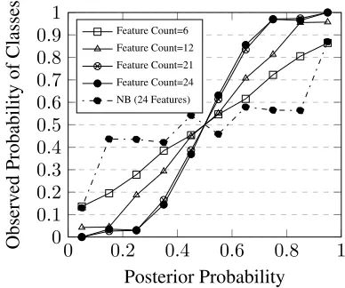
Feature Count=6 Feature Count=12 Feature Count=21 Feature Count=24 NB (24 Features)
Figure 4: Reliability diagram for a Perplexed Bayes classifier with the attenuation coefficient
[image:4.612.316.510.502.664.2]P(C|F) Points PB Acc Points NB Acc 0.5-0.6 387 0.6149 26 0.5000 0.6-0.7 421 0.8361 22 0.3636 0.7-0.8 439 0.9703 26 0.5000 0.8-0.9 300 0.9766 42 0.5238 0.9-1.0 43 1.0000 1474 0.8792
Table 1: Perplexed and Naive Bayes classifier ac-curacies for different confidence intervals (average of 24.4 features, and overall accuracy of 0.85).
0 0.2 0.4 0.6 0.8 1 0
0.1 0.2 0.3 0.4 0.5 0.6 0.7 0.8 0.9 1
Posterior Probability
Observ
ed
Probability
of
Classes
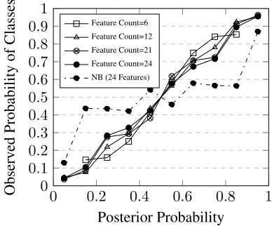
Feature Count=6 Feature Count=12 Feature Count=21 Feature Count=24 NB (24 Features)
Figure 5: Reliability diagram for a Perplexed Bayes classifier with the attenuation coefficient
optimized for good calibration a validation set, and a Naive Bayes (NB) curve for comparison.
In contrast, measurements for the Naive Bayes classifier, also shown in Table 1, indicate that 92.7%of the data points are classified with a con-fidence of above 0.9, and that the remaining data points are assigned to classes almost randomly, so the accuracy is not very sensitive to threshold changes between 0.5 and 0.9. Figure 3 shows an increase in the accuracy of classification with an increase in the posterior probability.
The reliability diagram for the Perplexed Bayes classifier with the Y-axis values representing the probability of a data point’s real class equalling the class for which the classifier’s posterior probabil-ity is plotted on the X-axis, is shown in Figure 4.
The reliability diagram in Figure 5 was obtained similarly using a Perplexed Bayes classifier where the attenuation coefficient was estimated so as to mimimize the Root Mean Square Error (RMSE) of the observed posterior probabilities from ideal values over a held-out validation set of data points. The RMSEs of the observed posterior proba-bilities of Figure 5 were0.069, 0.043, 0.049and
0 0.2 0.4 0.6 0.8 1 0.3
0.4 0.5 0.6 0.7 0.8 0.91
Posterior Probability Threshold
Precision
/Recall
Precision Female Precision Male Recall Female Recall Male
Figure 6: The precision and recall of the Perplexed Bayes classifier against decision thresholds.
0.064 for 6, 12, 21 and24 features respectively, whereas the RMSEs for a Naive Bayes classifier were0.016,0.093,0.173and0.164(at accuracies of71.5%,81.5%,85.7%and84.5%), establishing that on this data setthe Perplexed Bayes classifier produced better calibrated posterior probabilities for higher feature counts than a Naive Bayes clas-sifier of the same accuracy.
5.3 Precision & Recall Experiments
The precision and recall of the Perplexed Bayes classifier plotted against confidence thresholds for the selection of one class over the others are as shown in Figure 6.
6 Conclusions
We have shown that it is possible to build a clas-sifier (the Perplexed Bayes clasclas-sifier) that makes classification decisions that are identical to those of a Naive Bayes classifier without assuming that the features used are class-conditionally inde-pendent, by combining the class-conditional fea-ture probabilities into posterior probabilities using their geometric mean unlike the Naive Bayes sifier that takes their product, and that such a clas-sifier incorporating an attenuation coefficient can produce better calibrated posterior probabilities on the given data set than a Naive Bayes classifier for higher feature counts.
7 Future Work
We should like to see if the mathematics used in the Perplexed Bayes classifier could be used to make improvements to Hidden Markov Models and in Probabilistic Graphical Models.
[image:5.612.80.306.38.121.2] [image:5.612.81.275.191.352.2]Acknowledgments
The author is grateful to Srivatsan Laxman for the assistance he willingly offered with matters related to probability theory and mathematics, to Sumukh Ghodke for his feedback, and to the reviewers for their helpful and very useful comments.
References
Alexandru Niculescu-Mizil and Rich Caruana. 2005. Predicting good probabilities with supervised learn-ing. InProceedings of the 22nd international con-ference on Machine learning (ICML ’05),625–632.
Andrew McCallum and Kamal Nigam. 1998. A com-parison of event models for Naive Bayes text clas-sification. AAAI-98 workshop on learning for text categorization,752:41–48.
Antonio Bella and C`esar Ferri and Jos´e Hern´andez-Orallo and Mar¨ıa Jos´e Ram´ırez-Quintana. 2009. Similarity-binning Averaging: A Generalisation of Binning Calibration. In Proceedings of the 10th International Conference on Intelligent Data Engi-neering and Automated Learning (IDEAL’09),341– 349. Springer-Verlag.
Bianca Zadrozny and Charles Elkan. 2001. Obtaining calibrated probability estimates from decision trees and naive bayesian classiers.ICML, 609–616.
Bianca Zadrozny and Charles Elkan. 2002. Trans-forming classier scores into accurate multiclass probability estimates.KDD, 694–699.
Eibe Frank and Mark Hall and Bernhard Pfahringer. 2003. Locally Weighted Naive Bayes. In Proceed-ings of the Nineteenth Conference on Uncertainty in Artificial Intelligence, 249–256. Morgan Kaufmann Publishers Inc.
Fuchun Peng and Dale Schuurmans. 2003. Com-bining Naive Bayes and N-Gram Language Models for Text Classification. InProceedings ofThe 25th European Conference On lnformmion Retrieval Re-search (ECIR03).
Fuchun Peng and Dale Schuurmans and Shaojun Wang. 2004. Augmenting Naive Bayes Classifiers with Statistical Language Models.Information Retrieval, 7(3-4):317–345. Springer.
Geoffrey I. Webb and Michael J. Pazzani. 1998. Ad-justed probability naive Bayesian induction. In Pro-ceedings of the Eleventh Australian Joint Confer-ence on Artificial IntelligConfer-ence, 285–295. Springer-Verlag.
Harry Zhang. 2004. The Optimality of Naive Bayes. InProceedings of the Seventeenth Interna-tional Florida Artificial Intelligence Research Soci-ety Conference (FLAIRS 2004). AAAI Press.
Jason D. M. Rennie and Lawrence Shih and Jaime Tee-van and David R. Karger. 2003. Tackling the Poor Assumptions of Naive Bayes Text Classifiers. In
Proceedings of the Twentieth International Confer-ence on Machine Learning, 20:616–623.
Jochen Br¨ocker and Leonard A. Smith. 2007. In-creasing the Reliability of Reliability Diagrams. In
Weather and Forecasting, 22:651661.
John C. Platt. 1999. Probabilistic outputs for sup-port vector machines and comparisons to regular-ized likelihood methods.Advances in Large Margin Classiers, 61–74. MIT Press.
Khanh Nguyen, Brendan O’Connor. 2015. Posterior calibration and exploratory analysis for natural lan-guage processing models. Proceedings of EMNLP 2015.
Nayyar A. Zaidi and Jes´us Cerquides and Mark J. Car-man and Geoffrey I. Webb. 2013. Alleviating Naive Bayes Attribute Independence Assumption by At-tribute Weighting.Journal of Machine Learning Re-search, 14(1):1947–1988. JMLR.org.
Pat Langley and Stephanie Sage. 1994. Induction of Selective Bayesian Classifiers. Conference on Un-certainty in Artificial Intelligence, 399–406. Mor-gan Kaufmann.
Paul N. Bennett. 2000. Assessing the calibration of naive Bayes posterior estimates. Technical Report. Carnegie Mellon University.
Paul N. Bennett. 2003. Using Asymmetric Distri-butions to Improve Text Classifier Probability Es-timates. In Proceedings of the 26th Annual Inter-national ACM SIGIR Conference on Research and Development in Informaion Retrieval (SIGIR ’03), 111–118. ACM.
Rich Caruana and Alexandru Niculescu-Mizil. 2006. An Empirical Comparison of Supervised Learn-ing Algorithms. In Proceedings of the 23rd in-ternational conference on Machine learning (ICML ’06),161–168. ACM.
Stefan R¨uping. 2006. Robust Probabilistic Calibra-tion. InProceedings of the 17th European Confer-ence on Machine Learning, 743–750. Springer.
Susana Eyheramendy and David D. Lewis and David Madigan. 2003. On the Naive Bayes Model for Text Categorization. In9th International Workshop on Artificial Intelligence and Statistics.