Numerical Study of Burning of Biomass in Fixed Bed

ISSN Online: 1947-3818 ISSN Print: 1949-243X

DOI: 10.4236/epe.2019.112003 Feb. 21, 2019 35 Energy and Power Engineering

Numerical Study of Burning of Biomass in Fixed

Bed

Chamga Tchana Armand

, Obounou Akong

, Beguide Bonoma

1_{Unit for Research and Doctoral Studies in Physics and Applications, Postgraduate School of Science, Technology and Geoscience,}

University of Yaounde 1, Yaounde, Cameroon

2_{Department of Physics, Faculty of Sciences, University of Yaounde 1, Yaounde, Cameroon}

3_{Laboratory of Analysis of Energy Technologies and the Environment (LATEE), University of Yaounde 1, Yaounde, Cameroon} 4_{Department of Physics, ENS Yaounde, University of Yaounde 1, Yaounde, Cameroon}

Abstract

The combustion of biomass not only falls in energy production, but also in the recovery of waste. The treatment method most used for the recovery of waste is incineration because this method of treatment can minimize the vo-lume of waste. In this work, it comes to realize a numerical modeling of the combustion of biomass in a fixed grate furnace. A literature review allowed us to describe the stages of combustion in terms of mathematical equations. Taking into account the results of elemental analysis and immediate analysis, solid and gaseous species used to simulate their transport equations are: Dry fuel (biomass), char, CH4, O2, CO, H2O, CO2, and N2. From equations of

energy transportation, we deducted the TS temperature of the solid fuel bed and Tg of gas. Subsequently, we simulated the resolution 1-D transport equa-tions using a computer code written by us and this on the basis of mathemat-ical modeling of the transport equations. This 1-D unstationnary model takes into account the different stages of load transformation. In this calculation code, we used the explicit Euler method for space discretization, and for the time resolution, we used an implicit method which solves stiff problems of differential equations to ordinary derivatives. The results are satisfactory be-cause the calculated numerical profiles follow the experimental profiles, such as, the temperature profiles, the loss of mass of the fuel bed and the speed of propagation of the flame front.

Keywords

Multiphasic Combustion, Biomass, Modeling, Numerical Computation, Fixed Bed

How to cite this paper: Armand, C.T., Akong, O. and Bonoma, B. (2019) Numer-ical Study of Burning of Biomass in Fixed Bed. Energy and Power Engineering, 11, 35-57.

https://doi.org/10.4236/epe.2019.112003

Received: January 18, 2019 Accepted: February 18, 2019 Published: February 21, 2019

Copyright © 2019 by author(s) and Scientific Research Publishing Inc. This work is licensed under the Creative Commons Attribution International License (CC BY 4.0).

DOI: 10.4236/epe.2019.112003 36 Energy and Power Engineering

1. Introduction

Nowadays, the energies have an important place in the life of man and our cur-rent level of development requires an energy consumption increasingly growing. To meet this great need for energy, man has long had use of fossil fuels, rejecting into the atmosphere huge amounts of pollutants, including CO2. Given the need

to protect the environment by reducing the emission of greenhouse gases (GHGs), uncertainty about the uncertain future of fossil fuels, and especially our strong energy demand research have turned to new energy sources, which one of the main is combustion of biomass.

Renewable energies are numerous (biomass, solar, geothermal, waste, wind, hydraulic) and energy research grants them special attention. Here we focus es-pecially on the use of biomass as solid fuel that can be burned in a suitable oven to harness the energy released. The technologies used for burning biomass are numerous and the choice of a burner may depend on such factors as the nature of the fuel and its moisture content.

The combustion of biomass not only falls in energy production, but also in the recovery of waste. The treatment method most used for the recovery of waste is incineration because this method of treatment can minimize the volume of waste.

The multiphase combustion is a phenomenon that is part of our daily life: Cooking food using firewood or sawdust furnaces, incineration of household waste (HW), to name a few. This phenomenon, which seems simple, actually falls a physicochemical complexity. The multiphase combustion involves the phases solid, liquid and gaseous, noted, however, that obtaining a good combus-tion quality depends on the quality of fuel distribucombus-tion on the grid, on the turn-ing efficiency ensurturn-ing the best touch fuel/oxidizer to a sufficient temperature in drying zone-pyrolyse and on the nature of the fuel used. Several studies have al-ready been conducted in this area: This is the case of Shin and Choi [1] who are studying the burning of wood particles on fixed bed. Reaction rates are available in several chemical kinetic models [2]-[7]. Yann [8] presents the characteristics of fixed grate incinerators and Benkoussas et al.[9] are interested to thermal de-gradation of the wood particles.

This work is in search of a numerical method to solve equations, and for ap-proaching the experimental results. So we proposed writing a numerical compu-tation code that allows to numerically modeling the combustion of solid biomass particles. This numerical modeling is a combustion control to optimize the con-version of fuel into heat and reduce the production of pollutants. Controlling combustion involves controlling its various stages, namely drying, pyrolysis and combustion of the gases and the carbon residue released during the pyrolysis phase. One of the peculiarities of our numerical model is to use a stiff method for the resolution of the temporal part, which makes the numerical model more stable and more robust.

2. Combustion in Solid Fuel Bed

chem-DOI: 10.4236/epe.2019.112003 37 Energy and Power Engineering

ical reactions due to rapid oxidation of the fuel elements. The kinetics of the combustion of a load involves several stages from the drying to the heterogene-ous and homogeneheterogene-ous combustion.

On a smoldering wood particle (Figure 1), the main areas where the three preceding steps take place, can be observed (drying, pyrolysis, combustion of solid and gaseous phases). We can observe in this figure that the central section is made of raw wood and surrounded by a zone where the drying takes place. The following outer layer constitutes the pyrolysis zone and therefore devolatili-zation, and finally the last layer is the combustion zone of the carbonaceous re-sidue (coke plant).

Combustion is a complex process that involves several related equations to-gether and acting on two levels: In solid phase and gas phase.

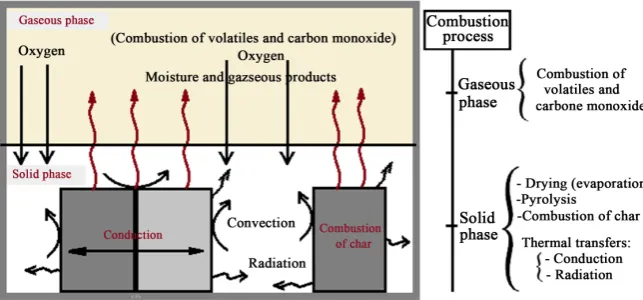
There is a significant interaction between the combustion in the solid phase and in the gas phase. This interaction is shown in Figure 2.

The main phenomena that take place in the solid phase are: drying or evapo-ration, pyrolysis and coal combustion. The heat transfer between solid particles here is by conduction and radiation. In this phase, the moisture produced during the drying as well as the volatiles produced during the pyrolysis and the carbon monoxide produced during the combustion of the coal will be returned to the gas phase. In the gas phase, there is therefore combustion of gaseous products from the solid phase. As another interaction, it is the gaseous phase that pro-vides the solid phase with the oxygen necessary for coal combustion, and the heat transfer between these two phases is by convection.

Figure 1. Representative section of burning wood particle.

DOI: 10.4236/epe.2019.112003 38 Energy and Power Engineering

The combustion process thus leads to the destruction of the solid fuel. During its degradation in an incinerator, or a burner, the solid fuel degrades in the presence of oxygen. This combustion results in a gradual decrease of the height of the solid fuel bed into the incinerator, as shown in Figure 3. The carbona-ceous residue obtained after the pyrolysis phase can also be gasified by steam or by the CO2 for subsequent use. After combustion, there is production of ashes

which are gradually cooled by the air injected into the bed always at room tem-perature.

Figure 3 which shows a schematic view of the process of combustion of the

wood particles in the fuel bed, one obtains the gradual decrease in height of the fuel bed.

To implement all these steps, here we have conducted a 1-D modeling of the combustion of the wood particles having a constant diameter and assumed the same for all particles.

3. Experimental Device

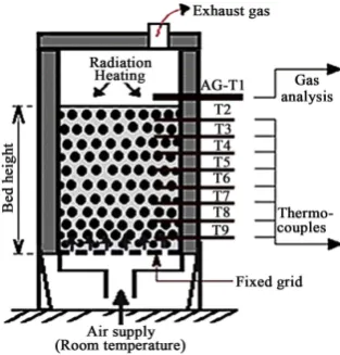
Figure 4 shows the experimental device. The combustion chamber of the device

is a cylinder of 18 cm internal diameter. It is thermally insulated by a refractory wall 3.5 cm thick, surrounded by an outer steel jacket of 0.3 cm thick. The grate to the base is perforated with holes to allow air entry.

Figure 3. Schematic of combustion in the solid fuel bed.

DOI: 10.4236/epe.2019.112003 39 Energy and Power Engineering

The fuel is made of wooden particles having a density ρ = 600 kg/m3_{, of radius}

of between 1 and 3 cm and its PCS is 19.8975 MJ/kg. The height of the fuel bed is 45 cm. The air enters under the grate at a speed of 0.05 m/s.

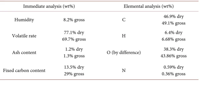
Table 1 presents the results of elemental and immediate analyzes of wood

particles used as fuel.

4. Mathematical Description of the Combustion Process

4.1. Conservation Equations

The conservation equations are written for solid and gaseous phases. These con-servation equations applied to a volume element can describe the instantaneous evolution of different variables anywhere in the field. One thus obtains transport equations whose general form is:

 convection term diffusion term

( )

u J S

t

ρ

_ρ

∅ ∅

+

∂ ∅ _{∇ ⋅ ∅ = ∇ ⋅ +}

∂   (1)

where ∅ represents the variables of mass, the total enthalpy (energy) or spe-cies; J∅ represents the broadcast stream, S∅ source terms, ρ the densities

of the solid or gaseous species and u the speeds of evolution of species. View test results in Table 1, the transport equations to solve are:

H2O:

(

) (

)

H O H O H O

,

b g g g b

b a eff g Y

Y Y Y

D R

t x x x

ε ρ

ρ ν

ε

ε

ρ

∂ ₊∂ ₌ ∂  ∂ ₊

 

∂ ∂ ∂ _ ∂ _ (2)

O2:

(

) (

)

O O O

,

b g g g b

b a eff g Y

Y Y Y

D R

t x x x

ε ρ

ρ ν

ε

ε

ρ

∂ ₊∂ ₌ ∂  ∂ ₊

 

∂ ∂ ∂ _ ∂ _ (3)

CH4:

(

) (

)

CH CH CH

,

b g g g b

b a eff g Y

Y Y Y

D R

t x x x

ε ρ

ρ ν

ε

ε

ρ

∂ ₊∂ ₌ ∂  ∂ ₊

 

∂ ∂ ∂ _ ∂ _ (4)

CO2:

(

) (

)

CO CO CO

,

b g g g b

b a eff g Y

Y Y Y

D R

t x x x

ε ρ

ρ ν

ε

ε

ρ

∂ ₊∂ ₌ ∂  ∂ ₊

 

∂ ∂ ∂ _ ∂ _ (5)

CO:

(

) (

)

,

b g g g b

b a eff g Y

Y Y _Y

D R

t x x x

ε ρ ρ ν ε

ε ρ

∂ ∂ _{∂  ∂ }

+ = _{ }+

∂ ∂ ∂  ∂  (6)

Table 1. Elementary and immediate analysis of fuel.

Immediate analysis (wt%) Elemental analysis (wt%)

Humidity 8.2% gross C _{49.1% gross} 46.9% dry

Volatile rate _{69.7% gross} 77.1% dry H _{6.68% gross} 6.4% dry

Ash content _{1.3% gross} 1.2% dry O (by difference) _{43.86% gross} 38.3% dry

DOI: 10.4236/epe.2019.112003 40 Energy and Power Engineering

N2:

(

) (

)

N N N

,

b g g g b

b a eff g

Y Y Y

D

t x x x

ε ρ

ρ ν

ε

ε

ρ

∂ ₊∂ ₌ ∂  ∂ 

 

∂ ∂ ∂ _ ∂ _ (7)

Energy Transport equation in:

Gas phase:

(

) (

)

(

)

b g pg g g g pg g b

g

g S g g lg

c T c T

t x

T

hS T T Q Q

x x

ε ρ ρ ν ε

λ ∂ ∂ + ∂ ∂ ∂   ∂ = _{ }+ − + + ∂ _ ∂ _ (8) Solid phase:

(

)

(

)

(

(

)

)

(

)

1 b s ps s 1 b s s ps s

s

eff g s s ls

c T c T

t x

T _{hS T T Q Q}

x x

ε ρ ε ρ ν

λ ∂ − ∂ − + ∂ ∂ ∂ ∂   = _{ }+ − + + ∂  ∂  (9) Humidity:

(

)

(

)

(

(

)

)

(

)

b s hum b s s hum

hum

b s s Y

Y Y

t x

Y

D R

x x

ε ρ ε ρ ν

ε ρ ∂ − ∂ − + ∂ ∂ ∂ ∂   = _ − _+ ∂  ∂  (10)

Dry solid fuel:

(

)

(

)

(

(

)

)

(

)

1 1

1 _Fuel

b s Fuel b s s Fuel

Fuel

b s s Y

Y Y

t x

Y

D R

x x

ε ρ ε ρ ν

ε ρ ∂ − ∂ − + ∂ ∂ ∂ ∂   = _ − _+ ∂  ∂  (11) Char:

(

)

(

)

(

(

)

)

(

)

b s char b s s char

char

b s s Y

Y Y

t x

Y

D R

x x

ε ρ ε ρ ν

ε ρ ∂ − ∂ − + ∂ ∂ ∂ ∂   = _ − _+ ∂  ∂  (12) Ash:

(

)

(

)

(

(

)

)

(

)

b s Ash b s s Ash

Ash

b s s Y

Y Y

t x

Y

D R

x x

ε ρ ε ρ ν

ε ρ ∂ − ∂ − + ∂ ∂ ∂ ∂   = _ − _+ ∂  ∂  (13)

Continuity equation in the gas phase: b

( )

(

)

ρ ρ ν

ε ∂ +ε ∂ =

∂ ∂ (14)

Continuity equation in the solid phase:

(

(

)

)

(

(

)

)

ε ρ ε ρ ν

∂ − ∂ −

+ =

∂ ∂

(15)

4.2. Modeling the Combustion of Solid Particles

During combustion of the wood particles, the phenomena of drying, pyrolysis, homogeneous and heterogeneous combustion act to reduce fuel in combustion products. The following equations will model these different physico-chemical phenomena.

4.2.1. Modeling of Drying

corres-DOI: 10.4236/epe.2019.112003 41 Energy and Power Engineering

ponds to the reaction:

Wet biomass→Dry biomass Moisture+ ₍₁₆₎

Drying the reaction rate is given by the Arrhenius equation [9] [10]:

e

vap s

Ea RT

vap vap h ap

R A Yρ

−

= ₍₁₇₎

where Avap, Eavap, TS, Yh and ρap are respectively the pre-exponential factor

( _{5.13 10}10

vap

A = × [11]), the activation energy (Eavap =88000 [11]), the

tem-perature of the solid, the mass fraction of water in the fuel and the density of wet biomass.

4.2.2. Modeling of Pyrolysis

Pyrolysis is the degradation of the organic portion of the dry fuel under the ef-fect of heat and leading to the formation of carbonaceous residue (coal) and the release of volatile gases. We have considered here for the process of thermal de-gradation of the wood particles in a two-step mechanism (blasi [12]):

 The first step corresponds to the production of volatile by the following reac-tion:

Solid fuel

→

Volatile

6

_

10700 5.6 10 exp

dev S Fuel

S

R M

T

− 

= × _{ }

  (19)

where MS Fuel_ is the mass of dry fuel present in each moment in the combus-tion chamber and TS the temperature of the solid fuel.

Here the volatile is supposed to be CH4 [1].

 The second step is the production of coal according to the reaction:

Solid fuel

→

Char

10

_

12800 2.66 10 exp

char S Fuel

S

R M

T

− 

= × _{ }

  (21)

4.2.3. Modeling of Homogeneous Combustion

Taking account of the elemental analysis of this solid fuel, the gaseous species that undergo homogeneous combustion (CH4, CO) burn according to the

reac-tions:

4 3 2 2

CH O CO 2H O

2

+ → + _{[14] (22)}

With the reaction rate [13] [14] [15]:

[

] [ ]

1 2 CH4 O2 exp

a b _a

g

g

E

R A

T

 

= _− _

  (23)

2 2

1

CO O CO

2

DOI: 10.4236/epe.2019.112003 42 Energy and Power Engineering

With the rate of reaction [17] [18]:

[ ][

] [ ]

2 3 CO H O O2 2 exp

a b _a

g

g

E

R A

T

 

= _− _

  (25)

α = 0.5 is a weighting factor, the average temperature Te to which the

reac-tion rate is calculated is given by [13] [19]:

(

)

e g s g s e g g s

T =αT + −α T T ≤T T =T T >T ₍₂₆₎

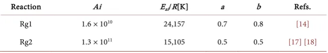
The constants Ai, E Rai (i = 2, 3, 4), a and b are given in Table 2.

4.2.4. Modeling of Heterogeneous Combustion

Char combustion may be described by the following two processes:

2 2 2

C O+ →CO and 2C O+ →2CO ₍₂₇₎

By combining these two equations, we obtain: [13]

(

)

(

)

2 2

C+ϕO →2 1−ϕ CO+ 2ϕ−1 CO (28) The constant ϕ _{is given by:}

(

)

2 2 1

f f

ϕ= +

+ (29)

where f is the CO/CO2 ratio (

2

CO CO

f = _{). It is given by [2]:}

3300 12e Ts

f

−

= ₍₃₀₎

The speed of the carbon combustion reaction is written as [20]:

( )

( ) 2

2

O

π _s

s

p C C C

d M k P

R = _ϕ (31)

where dp is the diameter of the particle, Mc the molar mass of carbon, PO2 the partial pressure of oxygen and kC_{( )s} the rate constant which is given by [20]:

( )

1

1 1

s

C

c act d

k

k k

=

+ Ω

(32)

This rate constant has three terms, namely:

→ _{The ash factor which takes into account the effect of the presence of ash on}

the oxidation kinetics and whose expression can be written [20]:

( )

( )

s

s

C act

C ash

Y

Y Y

Ω =

+ (33)

Table 2. Reaction parameters for the combustion of volatile.

Reaction Ai Eai/R[K] a b Refs.

Rg1 1.6 × 1010 _{24,157 0.7 0.8 [14]}

DOI: 10.4236/epe.2019.112003 43 Energy and Power Engineering

where YC_{( )s} and Yash are respectively the mass fractions of carbon residue

(char) and ash.

→ _{The rate constant due to chemical kinetics which is given by [10]:}

9000 1.175 e Ts

c s

k T

−

= ₍₃₄₎

where TS is the temperature of the solid.

→ _{The mass transfer coefficient} k_d which is defined by [20]:

2,m O d p ShD k d

= (35)

where DO_2,m is the mass diffusion coefficient of oxygen in air and Sh the

Sher-wood number defined by [21]:

0.5 1 3

2 0.6

Sh= + Re Sc ₍₃₆₎

where Sc is the Schmidt number given by:

2,m g g O Sc D µ ρ

= , and Re the Reynolds

number whose expression is: Re=ρg g pu d µg [22], where ug represents the

superficial gas velocity, µg the dynamic viscosity of the gas defined at the

temperature Tg of the gas by the expression [13]: 2 3 5 1.98 10 300 g g T

µ −  

   

= × (37)

And ρg the density of the gas calculated at the temperature of the gas phase

at a specific point of the bed; it is calculated according to the equation:

2 2 2 2 O N O N g g P Y Y RT M M ρ =   +       (38) 2 O

M and MN₂ are respectively the molar masses of dioxygen and

dinitro-gen, and P, the gas pressure. Taking air as the inlet gas, we have: YO2 =23.3%,

2

N 76.7%

Y = .

The Sherwood number can also be written [23]: 1 3

Sh JSc Re= ₍₃₉₎

where J which allows taking into account the diffusion of the gaseous mixture flowing through the fuel bed is the Colburn factor whose expression is [22] [23]:

0.82 0.368

1 0.765 0.365

b J Re Re ε   = _ + _

  (40)

With εb, the porosity of the fuel bed and the expression of which is:

,0 ,0 1 app b s ρ ε ρ

= − (41)

where ρapp,0 is the apparent density determined experimentally

( 3

,0 550 kg m

app

ρ = for wood particles), and ρs,0 the initial density of solid biomass particles estimated from the formula:

,0 _ 1 1 s b b dry water S Fuel

H H

ρ

ρ ρ

=

−

DOI: 10.4236/epe.2019.112003 44 Energy and Power Engineering

With Hb, the moisture on crude supplied by immediate analysis, ρwater the

density of water, and

ρ

The density of the solid during the thermal conversion is calculated from the following relationship: ( ) ( ) 1 s s C v Ash

water MV C s Ash

Y

Y Y

Yh

ρ

ρ ρ ρ ρ

=

+ + +

(43)

where Yh Y Y, v, C_{( )s} ,YAsh are respectively the mass fractions of moisture, volatile,

char and ash, and

ρ

ρ

ρ

ρ

vo-latiles, char and ash.

4.3. Transport Equations to Solve

The continuity equation for the gas phase is given by [15]:

( )

(

)

b _t b _x Rg

ρ ρ ν

ε ∂ +ε ∂ =

∂ ∂ (44)

The transport equation of the gaseous species is given by [13]:

(

) (

)

, ig

b g ig g g ig b ig

b a eff g Y

Y Y Y

D R

t x x x

ε ρ ρ ν ε

ε ρ

∂ ∂ ∂  ∂ 

+ =  +

∂ ∂ ∂ _ ∂ _ (45)

With ig = H2O, O2, CH4, CO2, CO, and N2.

The transport equation of the energy in the gas phase is given by [13] [15] [23]:

(

) (

)

₍

₎

g S g g lg

c T c T T

hS T T Q Q

t x x x

ε ρ ρ ν ε

λ

∂ ₊∂ ₌ ∂  ∂ _{+ − + +}

 

∂ ∂ ∂ _ ∂ _ (46)

where h is the heat transfer coefficient of gas-balance (W/m2_{K), S the specific}

exchange surface of the bed of particles (here S = 54 m2_/m3_{), Q}

g the heat gain due

to the combustion in gaseous phase (Qg =

∑

(

)

speed and the heat of reaction in the gas phase), and Qlg the loss of energy

(en-thalpy) along the bed wall. Qlgis given by [15]:

(

)

(

)

lg b g

Q =ε k L T T− ∆l (47) where k is the bed conductivity coefficient, L the length/height of the bed, T0 the

room temperature, and

∆

l

4.3.2. Equations of the Solid Phase

The continuity equation for the solid phase is given by [16]:

(

)

(

)

(

(

)

)

R

t x

ε ρ ε ρ ν

∂ − ∂ −

+ =

∂ ∂ (48)

The general form of the transport equation of solid species is given by [16]:

(

)

(

)

(

(

)

)

₍

₎

1 _is

b s is b s s is _is

b s s Y

Y Y _Y

D R

t x x x

ε ρ ε ρ ν

ε ρ

∂ − ∂ − _{∂  ∂ }

+ = _ − _+

DOI: 10.4236/epe.2019.112003 45 Energy and Power Engineering

where is = Humidity, dry fuel (solid biomass), char, ash.

The transport equation of the energy in the solid phase is given by [16]:

(

)

(

)

(

(

)

)

(

)

1 b s ps s 1 b s s ps s

s

eff g s s ls

c T c T

t x

T _{hS T T Q Q}

x x

ε ρ ε ρ ν

λ

∂ − ∂ −

+

∂ ∂

∂

∂  

= _{ }+ − + +

∂  ∂ 

(50)

Qs is the heat generation due to char combustion (W/m3) given by: s char char

Q =r x H∆ _where r_char and ∆Hchar represent speed and heat of reaction

of char combustion reaction in the solid phase. Qls is the loss of energy

(enthal-py) along the bed wall and is given by [15]:

(

)(

)(

)

ls b s

Q = −ε k L T T− ∆l ₍₅₁₎

where k is the bed conductivity coefficient, L the length/height of the bed, T0 the

room temperature, and ∆l the wall thickness.

In these transport equations, Ds represents the particle mixture coefficient

due to random movements of the particles in the bed, Da eff, the axial disper-sion coefficient which is given by [16]:

2,

, m 0.5

a eff O g p

D =D + v d ₍₅₂₎

And λeff the effective thermal conductivity coefficient given by [24]:

,0 0.5

eff eff gPrRe b

λ =λ + λ ε ₍₅₃₎

2,m

O

D is the mass diffusion coefficient of oxygen in the air, vg the gas

veloc-ity, and λeff,0 the conduction coefficient in the absence of gas flow.

The heat transfer coefficient by convection between the particles and the gas is:

g p

h Nu= λ d ₍₅₄₎

where λg is the thermal conductivity of the gas and is [13]:

4 0.717

4.8 10

g Tg

λ = × (55)

And Nu is the Nusselt number defined by:

0.625 0.33 2 b 0.295

Nu= ε + Re Pr (56)

where Pr is the Prandtl number which is written:

g pg g

Pr=µ C λ ₍₅₇₎

where cpg is the specific heat of the gas.

The reaction heats are derived from the formula:

,

d d

ig s reaction reaction

M

Q H

t

= ∆ ₍₅₈₎

where ∆Hr?action and ,

d d

ig s

M

t are respectively the enthalpy and the rate of the

DOI: 10.4236/epe.2019.112003 46 Energy and Power Engineering

4.4. Simplifying Assumptions

To solve these equations, we propose a number of assumptions including:

- The diffusion coefficients of temperature and species are assumed to be con-stant;

- Particles of solid biomass used as fuel are supposed to be dry, which allows us to neglect the drying step during the combustion modeling;

- The particles are assumed to average size, which allows us to accept the hy-pothesis of the diffusion regime [25].

4.5. System of Equations to Solve

The new system obtained after taking into account the above assumptions is:

 Transport equations of gas species:

( )

( )

, ig

ig ig ig

b g g g b b a eff g Y

Y Y Y

D R

t x x x

ε ρ ∂ +ρ ν ε ∂ =ε ρ ∂ _∂ _+

∂ ∂ ∂ _ ∂ _ (59)

where ig = {H2O, O2, CH4, CO2, CO, N2}.

 _{Transport equations of temperatures (energy):}

Gas Temperature:

g g g

b g pg g pg g b g g

T T T

c c Wt

t x x x

ε ρ ∂ +ρ ν ε ∂ =λ ∂ _∂ _+

∂ ∂ ∂ _ ∂ _ (60)

Temperature of the solid bed:

(

)

(

)

b s psc T_t b s s psc T_x eff _x T_x Wts

ε ρ ∂ ε ρ ν ∂ λ ∂ ∂ 

− + − = _{ }+

∂ ∂ ∂ _ ∂ _ (61)

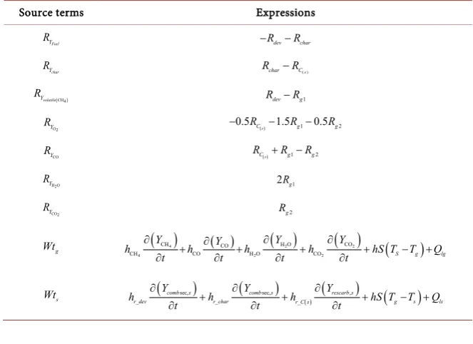
Table 3 gives the expressions of the source terms of transport equations based

on reaction rates.

Table 3. Summary of source terms of transport equations.

Source terms Expressions

Fuel Y

R −Rdev−Rchar

char Y

R Rchar−RC_{( )s}

(CH4)

volatile Y

R R_dev−R_g1

O2 Y

R −0.5RC( )s −1.5Rg1−0.5Rg2

CO Y

R RC( )s +Rg1−Rg2

H O2 Y

R 2Rg1

CO2 Y

R Rg2

g

Wt

( )

( )

( )

₍

₎

4 2 2

CH CO H O CO

CH CO H O CO S g lg

Y Y Y Y

h h h h hS T T Q

t t t t

∂ ∂ ∂ ∂

+ + + + − +

∂ ∂ ∂ ∂

s

Wt

(

)

(

)

(

)

₍

₎

_ _ _

comb s comb s rescarb s

r dev r char r C s g s ls

Y Y Y

h h h hS T T Q

t t t

∂ ∂ ∂

+ + + − +

DOI: 10.4236/epe.2019.112003 47 Energy and Power Engineering

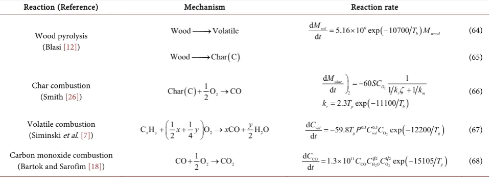
5. Summary of Reaction Equations

Table 4 summarizes the main reaction models used in our model.

6. Numerical Modeling

6.1. Numerical Methods

As a reminder, we have seen in the theoretical tools that all the equations we are trying to solve are of the form:

( )

0i i 1i i 1i i 1i i,

Y Y Y

a a b W Y t

t x x x

∂ _{= −} ∂ ₊ ∂ ∂ ₊  

∂ ∂ ∂ ∂  (62)

where Yi = {species (solid Yis or gaseous Yig), temperatures (of gaz Tg or of

solid bed Ts)}.

As numerical methods we use:

 An explicit method for space discretization and based on the explicit Euler: The Euler method is based on an explicit finite difference method. It allows approximating the derived differential equations. This method is widely used in programming because it provides great writing simplicity.

 An implicit method for the time resolution:

For solving the unstationnary term, we used an implicit method based on numerical differentiation formulas (NDFs) that solve stiff problems of differen-tial equations to ordinary derivatives. For this, we put the equation in the form:

( )

_{( )}

i Y F Y t ∂ =

∂ (63)

With F Y

( )

( )

(

)

( )

(

)

( )

6.2. Initial and Boundary Conditions

The initial conditions are as follows: The combustion process is initiated above the fuel bed. For this, the upper surface of the bed is exposed to a temperature of about 850˚C. This temperature is that of the source of ignition. The exposure of

Table 4. Summary of reaction models used in our model.

Reaction (Reference) Mechanism Reaction rate

Wood pyrolysis (Blasi [12])

Wood→Volatile d _{5.16 10 exp 10700}6 ( )

dvol b wood

M _{T M}

t = × − (64)

( )

Wood→Char C (65)

Char combustion

(Smith [26]) ( ) 2

1

Char C O CO

2

+ →

( )

2

2

d ₆₀ 1

d 1 1

2.3 exp 11100

char

O

r m

r p b

M _SC

t k k

k T T

ζ  = −

 ₊



= − (66)

Volatile combustion

(Siminski et al. [7]) C Hx y 1₂x 1₄y O2 xCO ₂yH O2

 

+_ + _ → +

  2

(

)

0.3 0.5 O

d _{59.8 exp 12200}

dvol g vol g

C _{T P C C T}

t = − − (67)

Carbon monoxide combustion

(Bartok and Sarofim [18]) 2 2

1

CO O CO

2

+ →

(

)

2 2

11 1 2 1 2

CO

CO H O O

d _{1.3 10 exp 15105}

d g

C _{C C C T}

DOI: 10.4236/epe.2019.112003 48 Energy and Power Engineering

the top of the bed at this temperature is done during a relatively short time ne-cessary for the appearance of the flame front that gradually spread in the fuel bed.

For solid and gaseous species, we consider here the mass fractions and calcu-lations are initialized at the onset of the flame front on the surface of the fuel bed.

Initial conditions (t = 0):

t = 0 and x = 0 (at the bottom of the fuel bed): Yis,0: YFuel,0 = 0.69; Ychar,0 = 0.1

and Yig,0: Yvolatile,0 = 10−2; Yo2,0 = 0.2; Yco,0 = 10−2; Yh2o,0 = 10−6; Yco2.0 = 10−6 et Yn2.0 = 0.747.

t = 0 and x < H: Tg,0 = TS,0 = T0 = 300 K, where H represents the height of the

fuel bed.

t = 0 and x = H (at the top of the fuel bed): Tg,0 = TS,0 = 1123 K.

Boundary conditions:

t > 0 and x = H (at the top of the fuel bed): d d 0

d d

is s

Y T

x = x = ; is = {dry fuel

(Solid biomass), char, ash} and d d 0

d d

ig g

Y T

x = x = ; ig = {H2O, O2, CH4, CO2, CO,

N2}.

7. Results and Discussion

The combustion process is initiated above the fuel bed. For this, the upper sur-face of the bed is exposed to a temperature of about 850˚C. This temperature is that of the source of ignition. The exposure of the top of the bed at this temper-ature is done during a relatively short time necessary for the appearance of the flame front that gradually spread in the fuel bed.

The combustion process is initiated above the fuel bed. For this, the upper surface of the bed is exposed to a temperature of about 850˚C. This temperature is that of the ignition source. The exposure of the surface of the bed at this temperature is for a fairly short time and necessary for the appearance of the flame front which will spread progressively in the fuel bed.

We have in Figure 4 the presentation of our burner. This burner is modeled on a model widely used in households. Figure 4 shows a modeling of said furnace, as well as the provision of thermocouples for measuring temperatures at different points. The thermocouple T9 (see Figure 4) is located 5 cm from the bottom of the oven, and the other thermocouples are spaced 5 cm each relative to the position of the other closest thermocouple.

The combustion process is performed in this burner, after introduction of the fuel. At the very beginning, the fuel (biomass) is introduced into the oven, up to a height of 45 cm. The fuel introduced is supposed to be initially at room temperature.

DOI: 10.4236/epe.2019.112003 49 Energy and Power Engineering

xposure temperature will cause pyrolysis of the fuel particles thus dried, allowing the release of volatiles and coal. These volatile gases will react in the gas phase. It follows a phenomenon of solid phase combustion of coal produced, and a gas phase combustion of volatiles (here mainly CH4) and CO produced during the

combustion of coal and CH4.

Figure 5 shows the temperature curves of the fuel bed. Figure 5(a) shows the

experimental results, Figure 5(b) is the one predicted by Shin & Choi [1], and

Figure 5(c) curve is the one predicted by our model.

(a)

(b)

(c)

DOI: 10.4236/epe.2019.112003 50 Energy and Power Engineering

Due to exposure to high temperatures of the upper surface of the fuel bed, the temperature in the bed increases rapidly, and the progression of the flame in the bed is gradually felt at the thermocouple T2 (see Figure 4 for its layout) which begins to heat up. At this time, the thermocouple T3 (respectively G3) located at 5 cm from T2 (respectively G3) remains almost always at room temperature, proof that the flame front has not yet arrived at this level. This weak progression of the flame front can be explained not only by the low conductivity of the fuel bed, but also by the supply air that always arrives at room temperature, thereby cooling the bed continuously. After a while, the temperature of thermocouple T3

(see Figure 5) explodes in its turn, and this same phenomenon is observed

successively for thermocouples T4 to T9 (respectively G4 to G9). The first peak of temperature is observed around 10 minutes, and the second peak of temperature, measured by the thermocouple T3, it meanwhile obtained around 18 minutes. The flame front progressively progresses to the bottom of the bed, leaving ash on its way. And when this flame front reaches the bed, then the fuel is completely transformed into ash and the combustion ends. The hot ash produced is cooled by the supply air, which explains the rapid temperature drop of thermocouple T9 (respectively G9) as shown in Figure 5(c) (respectively 5-a). The numerical temperature curves of thermocouples T2 to T9 have substantially the same ignition delays as the respective experimental curves G2 to G9 (see Figure 5). Referring to ignition delays, temperature peaks and also the shape of the temperature curves at the post-combustion phase, we can say that our numerical curves of temperature (see Figure 5(c)) seem to stick better with the experimental measurements (see Figure 5(a)).

Figure 6 shows the prediction curve by our model of the variation of the dry

fuel mass fraction (obtained after the drying phase). These curves are obtained for each observation point, and these points correspond here to the positions of the different thermocouples T2 to T9 as indicated in Figure 4.

DOI: 10.4236/epe.2019.112003 51 Energy and Power Engineering

For the position of thermocouple T2, we observe a first plateau up to about 10 minutes, at which time the mass fraction of dry fuel decreases sharply until it vanishes, proof that the pyrolysis process is complete. After this time, the mass fraction of dry fuel is kept at 0, thus forming a plateau again at this value. For the position of the thermocouple T3, the same phenomenon is observed with the only difference that the pyrolysis is carried out a little later, or about 18 minutes.This proves that the heat has progressed in the furnace, and that the rise in temperature due to this heat supply is already sufficient to cause the pyrolysis of our fuel.

This proves that the heat has progressed in the furnace, and that the rise in temperature due to this heat supply is already sufficient to cause the pyrolysis of our fuel. We then observe and successively the same phenomena for the points of observation of T4 to T9, and this at different times. These curves therefore have the same profile and differ only in the ignition delay. The lags between the ignition delays of these different profiles are due to the convection and diffusion phenomena that create a transport in the bed.

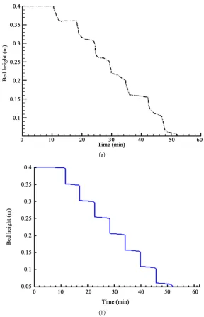
During the propagation of the flame front along the bed, there is degradation of the fuel with production of ash and energy, which causes a loss of mass. This loss of mass is characterized by a gradual decline in the volume or height of the bed during combustion. This decrease in bed height modeled in Figure 1 is shown in Figure 7. Figure 7(a) from Shin and Choi [1] presents the experimental results obtained by measuring the decrease in the height of the fuel bed, and Figure 7(b) shows the numerical results obtained at fixed observation points. These numerical and experimental results are similar.

The significant decrease in bed mass observed at each stage correspond to the temperature peaks observed previously, and these levels are due to the limited number of measuring or observation points. The loss of mass in the fuel bed is normal and can be explained by the transformation of the starting fuel into energy, ashes and burnt gases.

Figure 8 shows the speed of propagation of the flame front along the fuel bed,

a speed predicted by our model. We find that the flame front progresses steadily along the fuel bed. However, it should be noted that when the flame front arrives at the end of the bed (located 45 cm from the initial bed height), then the combustion stops, and the flame front is stopped at this position because not only the starting fuel is totally degraded and turned into ashes, but also the hot ashes produced are cooled by the air supply that always arrives at room temperature. As a result, the speed of propagation of the flame at the bed is therefore zero.

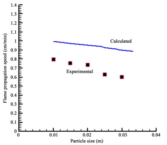
Figure 9 shows the influence of the size of the fuel particles on the propagation speed of the flame front.

DOI: 10.4236/epe.2019.112003 52 Energy and Power Engineering (a)

(b)

Figure 7. Loss of mass of the fuel bed: (a) measurement; (b) prediction.

DOI: 10.4236/epe.2019.112003 53 Energy and Power Engineering Figure 9. Effect of particle size on the propagation velocity of the flame front.

the particle size increases, the speed of propagation of the flame decreases. To explain this decrease in the propagation velocity of the flame front, we can say that when the particle size increases, the surface per unit mass decreases, and consequently the cooling effect of the air also decreases.In order to make the combustion stable, therefore, a higher maximum air ratio is required than in the case of smaller particles. Increasing the particle size therefore increases the drying time, and therefore the burning time of the fuel particles, and so the flame front evolves more slowly, which explains the decrease in flame front velocity when particle size increases, as shown in Figure 9.

8. Conclusions

The study of biomass combustion was carried out here on a fixed bed grid. For this study, we have modeled the different stages of solid combustion in terms of mathematical equations of evolution of species and energy. Multiphasic combustion is a physicochemical complexity. We used a 1-D model here. This 1-D modeling of the transport equations allowed us to propose a numerical model of multiphase combustion of biomass.

DOI: 10.4236/epe.2019.112003 54 Energy and Power Engineering

The distribution of the fuel on the grid, the size of the particle, the ignition temperature and also the supply air flow are important parameters for obtaining good combustion.

Here, the energy produced during combustion in the form of heat can be used for example in households for cooking meals, drying fruit, etc.

In view of the results obtained, and with some differences, we can say that our model reproduces the physico-chemical and heat transfer phenomena that occur during combustion in this fixed bed.

Conflicts of Interest

The authors declare no conflicts of interest regarding the publication of this paper.

References

[1] Shin, D. and Choi, S. (2000) The Combustion Of Simulated Waste Particules in a Fixed Bed. Combustion and Flame, 121, 167-180.

https://doi.org/10.1016/S0010-2180(99)00124-8

[2] Badzioch, S. and Hawksley, P.G.W. (1970) Kinetics of Thermal Decomposition of Pulverized Coal Particles. Industrial & Engineering Chemistry Process Design and Development, 9, 521-530. https://doi.org/10.1021/i260036a005

[3] Kobayashi, H., Howard, J.B. and Sarofim, A.F. (1977) Coal Devolatilization at High Temperatures. The Sixteenth Symposium (International) on Combustion, Massachusetts Institute of Technology, Cambridge, Massachusetts, 15-20 August 1976, Vol. 16, 411-425.

[4] Baum, M.M. and Street, P.J. (1971) Predicting the Combustion Behavior of Coal Particle. Combustion Science and Technology, 3, 231-243.

https://doi.org/10.1080/00102207108952290

[5] Fletcher, T.H., Kerstein, A.R., Pugmire, R.J. and Grant, D.M. (1990) Chemical Per-colation Model for Devolatilization: 2. Temperature and Heating Rate Effects on Product Yields. Energy and Fuels, 4, 54. https://doi.org/10.1021/ef00019a010

[6] Field, M.A. (1969) Rate of Combustion of Size-Graaded Fractions of Char from a Low Rank Coal between 1200 K - 2000 K. Combustion and Flame, 13, 237-252.

https://doi.org/10.1016/0010-2180(69)90002-9

[7] Siminski, V.J., Wright, F.J., Edelman, R.B., Economos, C. and Fortune, O.F. (1972) Research on Methods of Improving the Combustion Characteristics of Liquid Hy-drocarbon Fuels’. Rept. AFAPL TR 72-74, Vols. I and II, Air Force Aeropropulsion Laboratory, Wright Patterson Air Force Base, Dayton, Ohio.

[8] Rogaune, Y. (2005) Production de chaleur à partir du bois-Combustible et appareillage. Technique de l’ingénieur, BE 8 747, Vol. 1.

[9] Benkoussas, B., Consalvi, J.L., Porterie, B., Sardoy, N. and Loraud, J.C. (2007) Mod-elling Thermal Degradation of Woody Fuel Particles. International Journal of Thermal Sciences, 46, 319-327. https://doi.org/10.1016/j.ijthermalsci.2006.06.016

[10] Johansson, R., Thunman, H. and Leckner, B. (2007) Influence of Intraparticle Gra-dients in Modeling of Fixed Bed Combustion. Combustion and Flame, 149, 49-62.

https://doi.org/10.1016/j.combustflame.2006.12.009

DOI: 10.4236/epe.2019.112003 55 Energy and Power Engineering

Comparison of Different Models. Progress in Computational Fluid Dynamics, 6, 188-199. https://doi.org/10.1504/PCFD.2006.010027

[12] Blasi, C.D. (1993) Modeling and Simulation of Combustion Processes of Charring and Non-Charring Solid Fuels. Progress in Energy and Combustion Science, 19, 71-104. https://doi.org/10.1016/0360-1285(93)90022-7

[13] Zhou, H., Jensen, A.D., Glarborg, P., Jensen, P.A. and Kavaliauskas, A. (2005) Nu-merical Modeling of Straw Combustion in a Fixed Bed. Fuel, 84, 389-403.

https://doi.org/10.1016/j.fuel.2004.09.020

[14] Desroches-Ducarne, E.J., Dolignier, C., Marty, E., Martin, G. and Delfosse, L. (1998) Modelling of Gaseous Pollutants Emissions in Circulating Fluidized Bed Combustion of Municipal Refuse. Fuel, 77, 1399-1410.

https://doi.org/10.1016/S0016-2361(98)00060-X

[15] Kausley, S.B. and Pandit, A.B. (2010) Modelling for Solid Fuel Stoves. Fuel, 89, 782-791. https://doi.org/10.1016/j.fuel.2009.09.019

[16] Yang, Y.B., Goh, Y.R., Zakaria, R., Nasserzadeh, V. and Swithenbank, J. (2002) Ma-thematical Modeling of MSW Incineration on a Travelling Bed. Waste Manage-ment, 22, 369-380. https://doi.org/10.1016/S0956-053X(02)00019-3

[17] Howard, J.B., William, G.C. and Fine, D.H. (1973) Kinetics of Carbon Monoxide Oxidation in Postflame Gases. Symposium (International) on Combustion, 14, 975-986. https://doi.org/10.1016/S0082-0784(73)80089-X

[18] Bartok, W. and Sarofim, A. (1991) Fossil Fuel Combustion. John Wiley, New York. [19] Bryden, K.M. and Ragland, K. (1973) Numerical Modeling of a Deep, Fixed Bed

Combustor. Energy & Fuels, 10, 269-275. https://doi.org/10.1021/ef950193p

[20] Thunman, H. and Leckner, B. (2007) Thermo Chemical Conversion of Biomass and Wastes. Nordic Graduate School Biofuel GS-2, Chalmers, Goteborg, Sweden, 19-23 November 2007.

[21] Thunman, H. and Leckner, B. (2002) Thermal Conductivity of Wood—Models for Different Stages of Combustion. Biomass and Energy, 23, 47-54.

https://doi.org/10.1016/S0961-9534(02)00031-4

[22] Dwivedi, P.N. and Upadhyay, S.N. (1977) Particle-Fluid Mass Transfer in Fixed and Fluidized Beds. Industrial & Engineering Chemistry Process Design and Develop-ment, 16, 157-165. https://doi.org/10.1021/i260062a001

[23] Bruch, C. and Peter, B. and Nussbaumer, T. (2003) Modelling Wood Combustion under Fixed Bed Conditions. Fuel, 82, 729-738.

https://doi.org/10.1016/S0016-2361(02)00296-X

[24] Fjellerup, J., Henriksen, U., Jensen, A.D., Jensen, P. and Glarborg, P. (2003) Heat Transfer in a Fixed Bed of Straw Char. Energy & Fuels, 17, 1251-1258.

https://doi.org/10.1021/ef030036n

[25] Huttunen, M., KJäldman, L. and Saastamoinen, J. (2004) Analysis of Grate Firing of Wood with Numerical Flow Simulation. IFRF Combustion Journal, Article No. 200401.

DOI: 10.4236/epe.2019.112003 56 Energy and Power Engineering

Nomenclature

ig

Y : Mass fraction of the gas species i

is

Y : Mass fraction of solid species i s

u : Lowering speed of the solid fuel [m/s]

s

λ _{: Thermal conductivity of solid}

g

λ

g

µ _{: Dynamic viscosity of gas}

k: Bed conductivity coefficient

i

M : Molar mass of species i [g/mol]

g

u : Superficial gas velocity [m/s]

2

O

P : Partial pressure of oxygen [Pa]

i

f

h° _{: Enthalpy of formation of species i [J/mol]}

Lvap: Latent heat of vaporization of water [J/kg]

S: Exchange surface of the particles of the bed [m2_/m3_] i

D: Mass diffusion coefficient of species i

i

Y

R : Source term of the transport equation of species i g

Wt : Term source of the transport equation of Tg s

Wt : Term source of the transport equation of TS t: Time [s]

,0

ig

Y : Initial value of Yig

,0

is

Y : Initial value of Yis S

T : Temperature of solid [K]

g

T : Gas Temperature [K] ,0

S

T : Initial value of TS [K]

,0

g

T : Initial value of Tg [K] a

T : Ambient temperature [K]

ri

Q : Heat of the reaction ri [W]

b

ε _{: Porosity of fuel bed}

p

d : Particle diameter [m]

dx: Space step [m]

i

ρ _{: Density of body i [kg/m}3_]

h: Convective heat transfer coefficient [W/m2_K] s

H : Humidity on dry

b

H : Humidity on crude

a

E : Activation energy [J] _

r ri

h :Heat of the reaction ri [J/kg]

act

Ω _{: Ash Factor}

Greek letters

s

λ _{: Thermal conductivity of solid}

g

λ

g

µ _{: Dynamic viscosity of gas} ξ_{: Thermal conductivity of solid}

b

DOI: 10.4236/epe.2019.112003 57 Energy and Power Engineering i

ρ : Density of body i act

Ω _{: Ash Factor}

Abbreviations