Word and Document Embedding with vMF Mixture Priors on Context Word Vectors

Proceedings of the 57th Annual Meeting of the Association for Computational Linguistics, pages 3319–3328 3319

Word and Document Embedding with vMF-Mixture Priors on Context

Word Vectors

Shoaib Jameel

Medway School of Computing University of Kent [email protected]

Steven Schockaert

School of Computer Science and Informatics Cardiff University

[email protected]

Abstract

Word embedding models typically learn two types of vectors: target word vectors and con-text word vectors. These vectors are normally learned such that they are predictive of some word co-occurrence statistic, but they are oth-erwise unconstrained. However, the words from a given language can be organized in various natural groupings, such as syntactic word classes (e.g. nouns, adjectives, verbs) and semantic themes (e.g. sports, politics, sen-timent). Our hypothesis in this paper is that embedding models can be improved by explic-itly imposing a cluster structure on the set of context word vectors. To this end, our model relies on the assumption that context word vec-tors are drawn from a mixture of von Mises-Fisher (vMF) distributions, where the parame-ters of this mixture distribution are jointly op-timized with the word vectors. We show that this results in word vectors which are qualita-tively different from those obtained with exist-ing word embeddexist-ing models. We furthermore show that our embedding model can also be used to learn high-quality document represen-tations.

1 Introduction

Word embedding models are aimed at learning vector representations of word meaning (Mikolov et al.,2013b;Pennington et al.,2014;Bojanowski et al.,2017). These representations are primarily learned from co-occurrence statistics, where two words are represented by similar vectors if they tend to occur in similar linguistic contexts. Most models, such as Skip-gram (Mikolov et al.,2013b) and GloVe (Pennington et al.,2014) learn two dif-ferent vector representations w and w˜ for each wordw, which we will refer to as the target word vector and the context word vector respectively. Apart from the constraint thatwi·w˜j should re-flect how often words wi andwj co-occur, these

vectors are typically unconstrained.

As was shown in (Mu et al., 2018), after per-forming a particular linear transformation, the an-gular distribution of the word vectors that are ob-tained by standard models is essentially uniform. This isotropy property is convenient for study-ing word embeddstudy-ings from a theoretical point of view (Arora et al., 2016), but it sits at odds with fact that words can be organised in various nat-ural groupings. For instance, we might perhaps expect that words from the same part-of-speech class should be clustered together in the word em-bedding. Similarly, we might expect that organ-ising word vectors in clusters that represent se-mantic themes would also be beneficial. In fact, a number of approaches have already been proposed that use external knowledge for imposing such a cluster structure, capturing the intuition that words which belong to the same category should be rep-resented by similar vectors (Xu et al., 2014;Guo et al., 2015;Hu et al., 2015; Li et al.,2016c) or be located in a low-dimensional subspace (Jameel and Schockaert,2016). Such models tend to out-perform standard word embedding models, but it is unclear whether this is only because they can take advantage of external knowledge, or whether imposing a cluster structure on the word vectors is itself also inherently useful.

directional data (Banerjee et al.,2005).

We show that this results in word vectors that are qualitatively different from those obtained us-ing existus-ing models, significantly outperformus-ing them in syntax-oriented evaluations. Moreover, we show that the same model can be used for learning document embeddings, simply by view-ing the words that appear in a given document as context words. We show that the vMF distribu-tions in that case correspond to semantically co-herent topics, and that the resulting document vec-tors outperform those obtained with existing topic modelling strategies.

2 Related Work

A large number of works have proposed tech-niques for improving word embeddings based on external lexical knowledge. Many of these ap-proaches are focused on external knowledge about word similarity (Yu and Dredze, 2014; Faruqui et al., 2015;Mrksic et al., 2016), although some approaches for incorporating categorical knowl-edge have been studied as well, as already men-tioned in the introduction. What is different about our approach is that we do not rely on any external knowledge. We essentially impose the constraint that some category structure has to exist, without specifying what these categories look like.

The view that the words which occur in a given document collection have a natural cluster struc-ture is central to topic models such as Latent Dirichlet Allocation (LDA) (Blei et al.,2003) and its non-parametric counterpart called Hierarchi-cal Dirichlet Processes (HDP) (Teh et al., 2005), which automatically discovers the number of la-tent topics based on the characteristics of the data. In recent years, several approaches that com-bine the intuitions underlying topic models with word embeddings have been proposed. For exam-ple, in (Das et al.,2015) it was proposed to replace the usual representation of topics as multinomial distributions over words by Gaussian distributions over a pre-trained word embedding, while ( Bat-manghelich et al.,2016) and (Li et al.,2016b) used von Mises-Fisher distributions for this purpose. Note that documents are still modelled as multi-nomial distributions of topics in these models. In (He et al., 2017) the opposite approach is taken: documents and topics are represented as vectors, with the aim of modelling topic correlations in an efficient way, while each topic is represented as a

multinomial distribution over words. In this pa-per, we take a different approach for learning doc-ument vectors, by not considering any docdoc-ument- document-specific topic distribution. This allows us to repre-sent document vectors and (context) word vectors in the same space and, as we will see, leads to im-proved empirical results.

Apart from using pre-trained word embeddings for improving topic representations, a number of approaches have also been proposed that use topic models for learning word vectors. For example, (Liu et al., 2015b) first uses the standard LDA model to learn a latent topic assignment for each word occurrence. These assignments are then used to learn vector representations of words and top-ics. Some extensions of this model have been pro-posed which jointly learn the topic-specific word vectors and the latent topic assignment (Li et al., 2016a;Shi et al.,2017). The main motivation for these works is to learn topic-specific word repre-sentations. They are thus similar in spirit to multi-prototype word embeddings, which aim to learn sense-specific word vectors (Neelakantan et al., 2014). Our method is clearly different from these works, as our focus is on learning standard word vectors (as well as document vectors).

Regarding word embeddings more generally, the attention has recently shifted towards contex-tualized word embeddings based on neural lan-guage models (Peters et al., 2018). Such contex-tualized word embeddings serve a broadly simi-lar purpose as the aforementioned topic-specific word vectors, but with far better empirical perfor-mance. Despite their recent popularity, however, it is worth emphasizing that state-of-the-art meth-ods such as ELMO (Peters et al., 2018) rely on a concatenation of the output vectors of a neural language model with standard word vectors. For this reason, among others, the problem of learn-ing standard word vectors remains an important research topic.

3 Model Description

The GloVe model (Pennington et al.,2014) learns for each wordwa target word vectorwand a con-text word vectorw˜ by minimizing the following objective:

X

i,j xij6=0

where xij is the number of times wi andwj co-occur in the given corpus,biandbj˜ are bias terms andf(xij)is a weighting function aimed at reduc-ing the impact of sparse co-occurrence counts. It is easy to see that this objective is equivalent to maximizing the following likelihood function

P(D|Ω)∝ Y i,j xij6=0

N(logxij;µij, σ2)f(xij)

whereσ2 _{>0can be chosen arbitrarily,N means} the Normal distribution and

µij =wi·w˜j+bi+ ˜bj

Furthermore, D denotes the given corpus and Ω

refers to the set of parameters learned by the word embedding model, i.e. the word vectorswiandw˜j and the bias terms.

The advantage of this probabilistic formulation is that it allows us to introduce priors on the pa-rameters of the model. This strategy was recently used in the WeMAP model (Jameel et al.,2019) to replace the constant varianceσ2 by a varianceσ2_j that depends on the context word. In this paper, however, we will use priors on the parameters of the word embedding model itself. Specifically, we will impose a prior on the context word vectorsw˜, i.e. we will maximize:

Y

i,j xij6=0

N(logxij;µij, σ2)f(xij)_·Y

i

P(w˜i)

Essentially, we want the prior P(w˜i) to model the assumption that context word vectors are clus-tered. To this end, we use a mixture of von-Mises Fisher distributions. To describe this distribution, we begin with a von Mises-Fisher (vMF) distri-bution (Mardia and Jupp,2009;Hornik and Gr¨un, 2014), which is a distribution over unit vectors in

Rd that depends on a parameter θ ∈ Rd, where

dwill denote the dimensionality of the word vec-tors. The vMF density for x ∈ S_d (withS_d the d-dimensional unit hypersphere) is given by:

vmf(x|θ) = e

θ|_x

0F1(;d/2;||θ||

2

4 )

where the denominator is given by

0F1(;p;q) =

∞

X

n=0

Γ(p) Γ(p+n)

qn n!

which is commonly known as the confluent hyper-geometric function. Note, however, that we will not need to evaluate this denominator, as it simply acts as a scaling factor. The normalized vector_kθ_θk, forθ6=0, is the mean direction of the distribution, whilekθkis known as the concentration parame-ter. To estimate the parameterθfrom a given set of samples, we can use maximum likelihood (Hornik and Gr¨un,2014).

A finite mixture of vMFs, which we denote as movMF, is a distribution on the unit hypersphere of the following form (x∈ Sd_):

h(x|Θ) =

K X

k=1

ψkvmf(x|θk)

where K is the number of mixture components, ψk ≥ 0 for each k,

P

kψk = 1, and Θ =

(θ1, ..., θK). The parameters of this movMF dis-tribution can be computed using the Expectation-Maximization (EM) algorithm (Banerjee et al., 2005;Hornik and Gr¨un,2014).

Note that movMF is a distribution on unit vec-tors, whereas context word vectors should not be normalized. We therefore define the prior on con-text word vectors as follows:

P(w˜)∝h w˜ kwk˜ |Θ

Furthermore, we use L2 regularization to constrain the norm kwk˜ . We will refer to our model as CvMF.

In the experiments, following (Jameel et al., 2019), we will also consider a variant of our model in which we use a context-word specific variance σ_j2. In that case, we maximize the following:

Y

i,j xij6=0

N(logxij;µij, σj2)· Y

i

P(w˜i)·

Y

i

P(σ2_j)

where P(σ2_j) is modelled as an inverse-gamma distribution (NIG). Note that in this variant we do not use the weighting functionf(xij), as this was found to be unnecessary when using a context-word specific varianceσ2_j in (Jameel et al.,2019). We will refer this variant as CvMF(NIG).

xij then reflect how often wordj occurs in doc-umenti. Below we will experimentally compare this strategy with existing methods for learning document representations, focusing especially on approaches that are inspired by probabilistic topic models. Indeed, we can intuitively think of the vMF mixture components in our model as rep-resenting topics. While there have already been topic models that use vMF distributions in this way (Batmanghelich et al.,2016;Li et al.,2016b), our approach is different because we do not con-sider a document-level topic distribution, and be-cause we do not rely on pre-trained word embed-dings.

4 Experiments

In this section we assess the potential of our model both for learning word embeddings (Section 4.1) and for learning document embeddings (Section 4.2). Our implementation along with trained vec-tors is available online1.

4.1 Word Embedding Results

In this section, we describe the word embedding results, where we directly compare our model with the following baselines: GloVe (Pennington et al., 2014), Skipgram (Mikolov et al.,2013b) (denoted as SG), Continuous Bag of Words (Mikolov et al., 2013b) (denoted as CBOW), and the recently pro-posed WeMAP model (Jameel et al., 2019). We have used the Wikipedia dataset which was shared by Jameel et al. (2019), using the same vocab-ulary and preprocessing strategy. We report re-sults for 300-dimensional word vectors and we use

K = 3000 mixture components for our model.

As evaluation tasks, we use standard word anal-ogy and similarity benchmarks.

Analogy. Table 1 shows word analogy results for three datasets. First, we show results for the Google analogy dataset (Mikolov et al., 2013a) which is available from the GloVe project2 and covers a mix of semantic and syntactic relations. These results are shown separately in Table 1 as GsemandGsynrespectively. Second, we consider the Microsoft syntactic word analogy dataset3, which only covers syntactic relations and is re-ferred to asMSR. Finally, we show results for the

1

https://bit.ly/313U2ml 2

https://github.com/stanfordnlp/GloVe

3_{https://aclweb.org/aclwiki/Analogy (State of the art)}

50 300 1,000 3,000

0.58 0.6 0.62 0.64 0.66 0.68

vMF Mixtures

Accurac

y

GSem GSyn

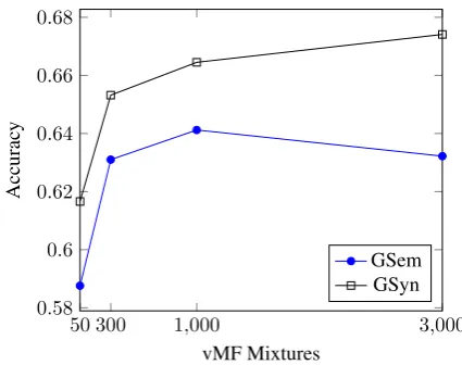
Figure 1: Accuracy vs number of vMF mixtures on the Google word analogy dataset for our model.

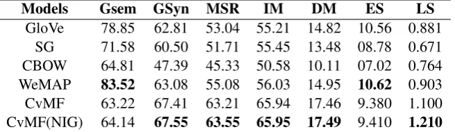
BATS analogy dataset4, which covers four cate-gories of relations: inflectional morphology (IM), derivational morphology (DM), encyclopedic se-mantics (ES) and lexicographic semantics (LS). The results in Table1clearly show that our model behaves substantially differently from the base-lines: for the syntactic/morphological relation-ships (Gsyn, MSR, IM, DM), our model outper-forms the baselines in a very substantial way. On the other hand, for the remaining, semantically-oriented categories, the performance is less strong, with particularly weak results for Gsem. ForES andIS, it needs to be emphasized that the results are weak for all models, which is partially due to a relatively high number of out-of-vocabulary words. In Figure1we show the impact of the num-ber of mixture componentsKon the performance for Gsem and Gsyn (for the NIG variant). This shows that the under-performance onGsemis not due to the choice of K. Among others, we can also see that a relatively high number of mixture components is needed to achieve the best results.

Word similarity. The word similarity results are shown in Table 2, where we have considered the same datasets as Jameel et al. (2019). In the table, we refer to EN-RW-Stanford as Stanf, EN-SIMLEX-999 as LEX, SimVerb3500 as Verb, EN-MTurk771 as Tr771, EN-MTurk287 as Tr287, EN-MENTR3K as TR3k, the RareWords dataset as RW, and the recently introduced Card-660 rare words dataset (Pilehvar et al., 2018) denoted as CA-660. Note that we have removed multi-word expressions from the RW-660 dataset and con-sider only unigrams, which reduces the size of

Models Gsem GSyn MSR IM DM ES LS

GloVe 78.85 62.81 53.04 55.21 14.82 10.56 0.881 SG 71.58 60.50 51.71 55.45 13.48 08.78 0.671 CBOW 64.81 47.39 45.33 50.58 10.11 07.02 0.764 WeMAP 83.52 63.08 55.08 56.03 14.95 10.62 0.903 CvMF 63.22 67.41 63.21 65.94 17.46 9.380 1.100 CvMF(NIG) 64.14 67.55 63.55 65.95 17.49 9.410 1.210

Table 1: Word analogy accuracy results on different datasets.

Models MC30 TR3k Tr287 Tr771 RG65 Stanf LEX Verb143 WS353 YP130 Verb RW CA-660

GloVe 0.739 0.746 0.648 0.651 0.752 0.473 0.347 0.308 0.675 0.582 0.184 0.422 0.301 SG 0.741 0.742 0.651 0.653 0.757 0.470 0.356 0.289 0.662 0.565 0.195 0.470 0.206 CBOW 0.727 0.615 0.637 0.555 0.639 0.419 0.279 0.307 0.618 0.227 0.168 0.419 0.219 WeMAP 0.769 0.752 0.657 0.659 0.779 0.472 0.361 0.303 0.684 0.593 0.196 0.480 0.301 CvMF 0.707 0.703 0.642 0.652 0.746 0.419 0.353 0.250 0.601 0.465 0.226 0.519 0.394 CvMF(NIG) 0.708 0.703 0.642 0.652 0.747 0.419 0.354 0.250 0.604 0.467 0.226 0.519 0.395

Table 2: Word similarity results on some benchmark datasets (Spearman’s Rho).

this dataset to 484 records. In most of these datasets, our model does not outperform the base-lines, which is to be expected given the conclusion from the analogy task that our model seems spe-cialized towards capturing morphological and syn-tactic features. Interestingly, however, in theRW andCA-660datasets, which focus on rare words, our model performs clearly better than the base-lines. Intuitively, we may indeed expect that the use of a prior on the context words acts as a form of smoothing, which can improve the representa-tion of rare words.

Qualitative analysis. To better understand how our model differs from standard word embed-dings, Table 3 shows the ten nearest neighbors (Al-Rfou et al., 2013) for a number of words ac-cording to our CvMF(NIG) model and acac-cording to the GloVe model. What can clearly be seen is that our model favors words that are of the same kind. For instance, the top 5 neighbours offastestare all speed-related adjectives. As an-other example, the top 7 neighbors ofred are col-ors. To further explore the impact of our model on rare words, Table 4 shows the nearest neigh-bors for some low-frequency terms. These exam-ples clearly suggest that our model captures the meaning of these words in a better way than the GloVe model. For example, the top neighbors of casioare highly relevant terms such asnotebook andcompute, whereas the neighbors obtained with the GloVe model seem largely unrelated. For com-parison, Table 5 shows the nearest neighbors of

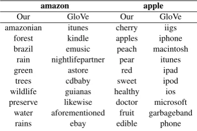
some high-frequency terms. In these case we can see that the GloVe model obtains the best results, as e.g.moreoveris found as a neighbor ofneural for our model, andindeedis found as a neighbor ofclouds. This supports the results from the sim-ilarity benchmarks that our model performs better than standard methods at modelling rare words but worse at modelling frequent words. Finally, Table 6shows the effect that our model can have on am-biguous words, where due to the use of the prior, a different dominant sense is found.

4.2 Document Embedding Results

To evaluate the document embeddings, we focus on two downstream applications: categorization and document retrieval. As an intrinsic evalua-tion, we also evaluate the semantic coherence of the topics identified by our model.

Document Categorization. We have evaluated our document embeddings on four standard doc-ument classification benchmarks: 1) 20 News-groups (20NG)5, 2) OHSUMED-23 (OHS)6, 3) TechTC-300 (TechTC)7, and 4) Reuters-21578 (Reu)8. As baselines, we consider the follow-ing approaches: 1) TF-IDF weighted bag-of-words representation, 2) LDA9, 3) HDP10, 4) the

5

http://qwone.com/ jason/20Newsgroups/ 6_{https://www.mat.unical.it/OlexSuite/Datasets/} SampleDataSets-download.htm

7_{http://techtc.cs.technion.ac.il/techtc300/techtc300.html} 8

https://archive.ics.uci.edu/ml/datasets/reuters-21578+text+categorization+collection

9

fastest india red attackers cession summer

Our GloVe Our GloVe Our GloVe Our GloVe Our GloVe Our GloVe

slowest fifth pakistan indian blue blue assailants assailants ceding ceding winter winter quickest second lanka mumbai yellow white attacker besiegers annexation ceded autumn olympics

slower sixth nepal pakistan white yellow townspeople pursuers annexing reaffirmation spring autumn faster slowest indian pradesh black which insurgents fortunately cede abrogation year spring fast ever bangladesh subcontinent green called policemen looters expropriation stipulating fall in surpassing quickest asia karnataka pink bright retaliation attacker continuance californios months beginning

next third delhi bengal gray pink rioters accomplices ceded renegotiation in next surpassed respectively sri bangalore well green terrorists captors incorporation expropriation also months

best tenth thailand asia the purple perpetrators strongpoints ironically zapatistas time during slow first china delhi with black whereupon whereupon dismantling annexation beginning year

Table 3: Nearest neighbors for selected words.

incisions unveil promissory batgirl casio

Our GloVe Our GloVe Our GloVe Our GloVe Our GloVe

incision incision unveiling unveils issuance estoppel catwoman huntress notebook <unk>

indentations embellishment utilise devise curiously scribbled nightwing zatanna compute nightlifepartner punctures preferably introduce unveiling wherein untraceable supergirl clayface practicality vgnvcm

scalpel notches invent <unk> handwritten evidencing batman superwoman utilizing counterstrike creases oftentimes expose finalise ostensibly gifting nemesis gcpd add graphing abrasions utilising publicize solidify purpotedly discordant abandon supergirl furthermore mkii lacerations lastly anticipating rediscover omnious renegotiation protege riddler utilising kajimitsuo extractions silhouettes unravelling embellish phony repossession unbeknownst woman utilizing reconditioned liposuction discreetly uncover reexamine proposing waiving reappears fight likewise bivort

apertures purposefully inaugrate memorializing ironically abrogation cyborg first anticipating spellbinder

Table 4: Nearest neighbors for low-frequency words.

neural clouds

Our GloVe Our GloVe

neuronal neuronal cloud cumulonimbus

brain cortical shadows cloud

cortical correlates mist obscured

perceptual neurons darkness mist

physiological plasticity heavens shadows

signaling neuroplasticity echoes aerosols

furthermore computation indeed sky

moreover circuitry furthermore fog

cellular spiking fog swirling

circuitry mechanisms lastly halos

Table 5: Nearest neighbors for high-frequency words.

amazon apple

Our GloVe Our GloVe

amazonian itunes cherry iigs

forest kindle apples iphone

brazil emusic peach macintosh

rain nightlifepartner pear itunes

green astore red ipad

trees cdbaby sweet ipod

wildlife guianas healthy ios

preserve likewise doctor microsoft

water aforementioned fruit garbageband

rains ebay edible phone

Table 6: Nearest neighbors for ambiguous words.

von Mises-Fisher clustering model (movMF)11, 5) Gaussian LDA (GLDA)12 and 6) Spherical HDP

11

https://cran.r-project.org/web/packages/movMF/index.html 12_{https://github.com/rajarshd/Gaussian LDA}

Models 20NG OHS TechTC Reu

TF-IDF 0.852 0.632 0.306 0.319 LDA 0.859 0.629 0.305 0.323 HDP 0.862 0.627 0.304 0.339 movMF 0.809 0.610 0.302 0.336 GLDA 0.862 0.629 0.305 0.352 sHDP 0.863 0.631 0.304 0.353 GloVe 0.852 0.629 0.301 0.315 WeMAP 0.855 0.630 0.306 0.345 SG 0.853 0.631 0.304 0.341 CBOW 0.823 0.629 0.297 0.339

CvMF 0.871 0.633 0.305 0.362

CvMF(NIG) 0.871 0.633 0.305 0.363

Table 7: Document classification results (F1).

(sHDP)1314, 7) GloVe15(Pennington et al.,2014), 8) WeMAP (Jameel et al., 2019), 9) Skipgram (SG) and Continuous Bag-of-Words16 (Mikolov et al., 2013b) models. In the case of the word embedding models, we create document vectors in the same way as we do for our model, by simply replacing the role of target word vectors with doc-ument word vectors.

In all the datasets, we removed punctuation and

13

https://github.com/Ardavans/sHDP 14

We do not compare with the method proposed in (Li et al., 2016b) because its implementation is not available. Moreover the sHDP method, which was published around the same time, is very similar in spirit, but the latter uses a nonparametric HDP topic model.

15

non-ASCII characters. We then segmented the sentences using Perl. In all models, parameters were tuned based on a development dataset. To this end, we randomly split our dataset into 60% training, 20% development and 20% testing. We report the results in terms of F1 score on the test set, using the Perf tool17_{. The trained document} vectors were used as input to a linear SVM classi-fier whose trade-off parameterCwas tuned from a pool of{10, 50, 100}, which is a common setting in document classification tasks. Note that our ex-perimental setup is inherently different from those setups where a word embedding model is evalu-ated on the text classification task using deep neu-ral networks, as our focus is on methods that learn document vectors in an unsupervised way. We have therefore adopted a setting where document vectors are used as the input to an SVM classifier. In our model, we have set the number of word embeddings iterations to 50. The parameters of the vMF mixture model were re-computed after every 5 word embedding iterations. We tuned the dimensionality of the embedding from the pool {100, 150, 200}and the number of vMF mixture components from the pool{200, 500, 800}.

We used the default document topic priors and word topic priors in the LDA and the HDP topic models. For the LDA model, we tuned the number of topics from the pool{50, 80, 100}and the num-ber of iterations of the sampler was set to 1000. We also verified in initial experiments that having a larger number of topics than 100 did not allow for better performance on the development data. The number of vMF mixtures of the comparative method, movMF, was tuned from the pool {200, 500, 800}. For GLDA, as in the original paper, we have used word vectors that were pre-trained using Skipgram on the English Wikipedia. We have tuned the word vectors size and number of topics from a pool of {100, 150, 200} and {50, 80, 100} respectively. The number of iterations of the sampler was again set to 1000. We have used same pre-trained word embeddings for sHDP, where again the number of dimensions was auto-matically tuned.

Table7summarizes our document classification results. It can be seen that our model outperforms all baselines, except for the TechTC dataset, where the results are very close. Among the baselines, sHDP achieves the best performance.

Interest-17_{http://osmot.cs.cornell.edu/kddcup/software.html}

Models WT2G HARD AQUT OHS

TF-IDF 0.288 0.335 0.419 0.432 LDA 0.291 0.346 0.447 0.461 HDP 0.301 0.333 0.436 0.455 movMF 0.255 0.311 0.421 0.432 GLDA 0.301 0.351 0.447 0.462 sHDP 0.301 0.334 0.437 0.452 GloVe 0.301 0.333 0.436 0.459 WeMAP 0.302 0.362 0.447 0.465 SG 0.301 0.345 0.447 0.461 CBOW 0.299 0.323 0.441 0.459 CvMF 0.305 0.361 0.449 0.469 CvMF(NIG) 0.306 0.363 0.450 0.471

Table 8: Document retrieval learning experiments (NDCG@10).

ingly, this model also uses von Mishes-Fisher mix-tures, but relies on a pre-trained word embedding.

Document Retrieval. Next we describe our doc-ument retrieval experiments. Specifically, we con-sider this problem as a learning-to-rank (LTR) task and use standard information retrieval (IR) tools to present our evaluation results.

We have used the following standard IR bench-mark datasets: 1) WT2G18 along with standard relevance assessments and topics (401 -450), 2) TREC HARD (denoted as HARD)19, 3) AQUAINT-2 (AQUT)20 where we considered only the document-level relevance assessments, and 4) LETOR OHSUMED (OHS)21_{, which} con-sists of 45 features along with query-document pairs with relevance judgments in five folds. We have obtained the raw documents and queries22 of this dataset, from which we can learn the doc-ument representations. As baselines, we have considered the following methods: 1) TF-IDF, 2) LDA (Blei et al.,2003), 3) HDP (Teh et al.,2005), 4) movMF (Banerjee et al.,2005), 5) sHDP ( Bat-manghelich et al., 2016), 6) GloVe (Pennington et al.,2014), 7) WeMAP (Jameel et al.,2019), 8) Skip-gram, and 9) CBOW word embedding mod-els (Mikolov et al.,2013b).

We have adopted the same preprocessing strat-egy as for the categorization task, with the excep-tion of OHSUMED, for which suitable LTR fea-tures are already given. For all other datasets we

18

http://ir.dcs.gla.ac.uk/test collections/access to data.html 19_{https://trec.nist.gov/data/hard.html}

20

https://catalog.ldc.upenn.edu/LDC2008T25 21

https://www.microsoft.com/en-us/download/details.aspx?id=52482

used the Terrier LTR framework23to generate the six standard LTR document features as described in (Jameel et al., 2015). The document vectors were then concatenated with these six features24. To perform the actual retrieval experiment, we used RankLib25 with a listwise RankNet (Burges et al.,2005) model26_{. Our results are reported in} terms of NDCG@10, which is a common evalua-tion metric for this setting.

Our training strategy is mostly the same as for the document categorization experiments, al-though for some parameters, such as the number of topics and vMF mixture components, we used larger values, which is a reflection of the fact that the collections used in this experiment are sub-stantially larger and tend to be more diverse (Wei and Croft, 2006). In particular, the word vector lengths were chosen from a pool of {150, 200, 300}and the vMF mixtures from a pool of{300, 1000, 3000}. In the LDA model, we selected the number of topics from a pool of{100, 150, 200}. For GLDA we have used the same pool for the number of topics. All our results are reported for five-fold cross validation, where the parameters of the LTR model were automatically tuned, which is a common LTR experimental setting (Liu et al., 2015a).

The results are presented in Table 8, showing that our model is able to consistently outperform all methods. Among the baselines, our NIG vari-ant achieves the best performance in this case, which is remarkable as this is also a word embed-ding model.

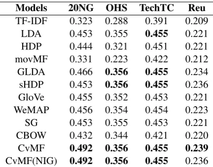
Word Coherence. In traditional topic models such as LDA, the topics are typically labelled by the k words that have the highest probability in the topic. These words tend to reflect semanti-cally coherent themes, which is an important rea-son for the popularity of topic models. Accord-ingly, measuring the coherence of the top-kwords that are identified by a given topic model, for each topic, is a common evaluation measure (Shi et al., 2017). Using the configurations that performed best on the tuning data in the document catego-rization task above, we used Gensim27 (Reh˚uˇrekˇ

23_{http://terrier.org/docs/v4.0/learning.html} 24

Note that in OHS the document vectors were concate-nated with 45 LTR features.

25

https://sourceforge.net/p/lemur/wiki/RankLib/ 26

Note that in principle any LTR model for IR could be used.

27_{radimrehurek.com/gensim/models/coherencemodel.html}

Models 20NG OHS TechTC Reu

TF-IDF 0.323 0.288 0.391 0.209 LDA 0.453 0.355 0.455 0.221 HDP 0.444 0.321 0.451 0.221 movMF 0.331 0.223 0.422 0.212 GLDA 0.466 0.356 0.455 0.234 sHDP 0.453 0.356 0.455 0.236 GloVe 0.455 0.352 0.453 0.221 WeMAP 0.456 0.354 0.454 0.223 SG 0.453 0.355 0.453 0.221 CBOW 0.432 0.344 0.421 0.220

CvMF 0.492 0.356 0.455 0.239

CvMF(NIG) 0.492 0.356 0.455 0.236

Table 9: Word coherence results in c v computed using Gensim.

and Sojka,2010) to compute the coherence of the top-20 words using the c v metric (R¨oder et al., 2015). For our model, GDLA and sHDP, the mixture components that were learned were con-sided as topics for this experiment. For GloVe, WeMAP, SG, TF-IDF, and CBOW, we used the von Mises-Fisher (vMF) soft clustering model (Banerjee et al., 2005) to determine the cluster memberships of the context words. For the TF-IDF results, we instead used hard vMF clustering (Hornik and Gr¨un, 2014), as the movMF results are based on TF-IDF features as well. We tuned the number of clusters using the tuning data. The top-20 words after applying the clustering model were then output based on the distance from the cluster centroid.

The results are shown in Table9, showing that the word clusters defined by our mixture compo-nents are more semantically coherent than the top-ics obtained by the other methods.

5 Conclusions

standard word embedding models when it comes to modelling rare words.

Word embedding models can also be used to learn document embeddings, by replacing word-word occurrences by document-word co-occurrences. This allowed us to compare our model with existing approaches that use von Mises-Fisher distributions for document mod-elling. In contrast to our method, these mod-els are based on topic modmod-els (e.g. they typically model documents as a multinomial distribution over topics). Surprisingly, we found that the doc-ument representations learned by our model out-perform these topic modelling-based approaches, even those that rely on pre-trained word embed-dings and thus have an added advantage, consid-ering that our model in this setting is only learned from the (often relatively small) given document collection. This finding puts into question the value of document-level topic distributions, which are used by many document embedding methods (being inspired by topic models such as LDA).

Acknowledgments

Steven Schockaert is supported by ERC Starting Grant 637277.

References

Rami Al-Rfou, Bryan Perozzi, and Steven Skiena. 2013. Polyglot: Distributed word representations for multilingual nlp. In Proceedings of the Seven-teenth Conference on Computational Natural Lan-guage Learning, pages 183–192, Sofia, Bulgaria. Association for Computational Linguistics.

Sanjeev Arora, Yuanzhi Li, Yingyu Liang, Tengyu Ma, and Andrej Risteski. 2016. A latent variable model approach to pmi-based word embeddings. Transac-tions of the Association for Computational Linguis-tics, 4:385–399.

Arindam Banerjee, Inderjit S Dhillon, Joydeep Ghosh, and Suvrit Sra. 2005. Clustering on the unit hyper-sphere using von mises-fisher distributions. Journal of Machine Learning Research, 6:1345–1382.

Kayhan Batmanghelich, Ardavan Saeedi, Karthik Narasimhan, and Sam Gershman. 2016. Nonpara-metric spherical topic modeling with word embed-dings. In Proceedings ACL, volume 2016, pages 537–542.

David M Blei, Andrew Y Ng, and Michael I Jordan. 2003. Latent Dirichlet allocation. Journal of ma-chine Learning research, 3:993–1022.

Piotr Bojanowski, Edouard Grave, Armand Joulin, and Tomas Mikolov. 2017. Enriching word vectors with subword information. Transactions of the Associa-tion for ComputaAssocia-tional Linguistics, 5:135–146.

Christopher Burges, Tal Shaked, Erin Renshaw, Ari Lazier, Matt Deeds, Nicole Hamilton, and Gre-gory N Hullender. 2005. Learning to rank using gra-dient descent. InProceedings of the 22nd Interna-tional Conference on Machine learning (ICML-05), pages 89–96.

Rajarshi Das, Manzil Zaheer, and Chris Dyer. 2015. Gaussian LDA for topic models with word embed-dings. InProceedings ACL, pages 795–804.

Manaal Faruqui, Jesse Dodge, Sujay Kumar Jauhar, Chris Dyer, Eduard H. Hovy, and Noah A. Smith. 2015. Retrofitting word vectors to semantic lexi-cons. InProceedings of NAACL, pages 1606–1615.

S. Guo, Q. Wang, B. Wang, L. Wang, and L. Guo. 2015. Semantically smooth knowledge graph embedding. InProceedings ACL, pages 84–94.

Junxian He, Zhiting Hu, Taylor Berg-Kirkpatrick, Ying Huang, and Eric P Xing. 2017. Efficient correlated topic modeling with topic embedding. In Proceed-ings of the 23rd ACM SIGKDD International Con-ference on Knowledge Discovery and Data Mining, pages 225–233.

Kurt Hornik and Bettina Gr¨un. 2014. movMF: An R package for fitting mixtures of von mises-fisher dis-tributions. Journal of Statistical Software, 58(10):1– 31.

Zhiting Hu, Poyao Huang, Yuntian Deng, Yingkai Gao, and Eric P. Xing. 2015. Entity hierarchy embedding. InACL, pages 1292–1300.

Shoaib Jameel, Zihao Fu, Bei Shi, Wai Lam, and Steven Schockaert. 2019. Word embedding as max-imum a posteriori estimation. InProceedings of the AAAI Conference on Artificial Intelligence.

Shoaib Jameel, Wai Lam, and Lidong Bing. 2015. Su-pervised topic models with word order structure for document classification and retrieval learning. In-formation Retrieval Journal, 18(4):283–330.

Shoaib Jameel and Steven Schockaert. 2016. Entity embeddings with conceptual subspaces as a basis for plausible reasoning. InProceedings of ECAI, pages 1353–1361.

Shaohua Li, Tat-Seng Chua, Jun Zhu, and Chunyan Miao. 2016a. Generative topic embedding: a con-tinuous representation of documents. In Proceed-ings ACL.

Yuezhang Li, Ronghuo Zheng, Tian Tian, Zhiting Hu, Rahul Iyer, and Katia P. Sycara. 2016c. Joint em-bedding of hierarchical categories and entities for concept categorization and dataless classification. In

Proceedings COLING, pages 2678–2688.

Quan Liu, Hui Jiang, Si Wei, Zhen-Hua Ling, and Yu Hu. 2015a. Learning semantic word embeddings based on ordinal knowledge constraints. In Pro-ceedings of ACL, pages 1501–1511.

Yang Liu, Zhiyuan Liu, Tat-Seng Chua, and Maosong Sun. 2015b. Topical word embeddings. In Proceed-ings AAAI, pages 2418–2424.

Kanti V Mardia and Peter E Jupp. 2009. Directional statistics, volume 494. John Wiley & Sons.

Tomas Mikolov, Kai Chen, Greg Corrado, and Jef-frey Dean. 2013a. Efficient estimation of word representations in vector space. arXiv preprint arXiv:1301.3781.

Tomas Mikolov, Ilya Sutskever, Kai Chen, Gregory S. Corrado, and Jeffrey Dean. 2013b. Distributed rep-resentations of words and phrases and their compo-sitionality. In Proceedings of NIPS, pages 3111– 3119.

Nikola Mrksic, Diarmuid ´O S´eaghdha, Blaise Thom-son, Milica Gasic, Lina Maria Rojas-Barahona, Pei-Hao Su, David Vandyke, Tsung-Hsien Wen, and Steve J. Young. 2016. Counter-fitting word vectors to linguistic constraints. In Proceedings NAACL-HLT, pages 142–148.

Jiaqi Mu, Suma Bhat, and Pramod Viswanath. 2018. All-but-the-top: Simple and effective postprocess-ing for word representations. InProceedings ICLR.

Arvind Neelakantan, Jeevan Shankar, Alexandre Pas-sos, and Andrew McCallum. 2014. Efficient non-parametric estimation of multiple embeddings per word in vector space. InProceedings of the 2014 Conference on Empirical Methods in Natural Lan-guage Processing, pages 1059–1069.

Jeffrey Pennington, Richard Socher, and Christo-pher D. Manning. 2014. GloVe: Global vectors for word representation. InProceedings of EMNLP, pages 1532–1543.

Matthew E. Peters, Mark Neumann, Mohit Iyyer, Matt Gardner, Christopher Clark, Kenton Lee, and Luke Zettlemoyer. 2018. Deep contextualized word rep-resentations. InProceedings of NAACL-HLT, pages 2227–2237.

Mohammad Taher Pilehvar, Dimitri Kartsaklis, Vic-tor Prokhorov, and Nigel Collier. 2018. Card-660: Cambridge rare word dataset-a reliable benchmark for infrequent word representation models. arXiv preprint arXiv:1808.09308.

Radim ˇReh˚uˇrek and Petr Sojka. 2010. Software Frame-work for Topic Modelling with Large Corpora. In

Proceedings of the LREC 2010 Workshop on New Challenges for NLP Frameworks, pages 45–50, Val-letta, Malta. ELRA. http://is.muni.cz/

publication/884893/en.

Michael R¨oder, Andreas Both, and Alexander Hinneb-urg. 2015. Exploring the space of topic coherence measures. InProceedings of the eighth ACM inter-national conference on Web search and data mining, pages 399–408. ACM.

Bei Shi, Wai Lam, Shoaib Jameel, Steven Schockaert, and Kwun Ping Lai. 2017. Jointly learning word embeddings and latent topics. In Proceedings SI-GIR, pages 375–384.

Yee W Teh, Michael I Jordan, Matthew J Beal, and David M Blei. 2005. Sharing clusters among re-lated groups: Hierarchical dirichlet processes. In

Advances in neural information processing systems, pages 1385–1392.

Xing Wei and W Bruce Croft. 2006. Lda-based doc-ument models for ad-hoc retrieval. InProceedings of the 29th annual international ACM SIGIR confer-ence on Research and development in information retrieval, pages 178–185. ACM.

C. Xu, Y. Bai, J. Bian, B. Gao, G. Wang, X. Liu, and T.-Y. Liu. 2014. RC-NET: A general framework for incorporating knowledge into word representations. InProc. CIKM, pages 1219–1228.