Stochastic Lexicalized Inversion Transduction Grammar for Alignment

Stochastic Lexicalized Inversion Transduction Grammar for Alignment

Hao Zhang and Daniel Gildea

Computer Science Department University of Rochester

Rochester, NY 14627

Abstract

We present a version of Inversion Trans-duction Grammar where rule probabili-ties are lexicalized throughout the syn-chronous parse tree, along with pruning techniques for efficient training. Align-ment results improve over unlexicalized ITG on short sentences for which full EM is feasible, but pruning seems to have a negative impact on longer sentences.

1 Introduction

The Inversion Transduction Grammar (ITG) of Wu (1997) is a syntactically motivated algorithm for producing word-level alignments of pairs of transla-tionally equivalent sentences in two languages. The algorithm builds a synchronous parse tree for both sentences, and assumes that the trees have the same underlying structure but that the ordering of con-stituents may differ in the two languages.

This probabilistic, syntax-based approach has in-spired much subsequent reasearch. Alshawi et al. (2000) use hierarchical finite-state transducers. In the tree-to-string model of Yamada and Knight (2001), a parse tree for one sentence of a transla-tion pair is projected onto the other string. Melamed (2003) presents algorithms for synchronous parsing with more complex grammars, discussing how to parse grammars with greater than binary branching and lexicalization of synchronous grammars.

Despite being one of the earliest probabilistic syntax-based translation models, ITG remains state-of-the art. Zens and Ney (2003) found that the con-straints of ITG were a better match to the decod-ing task than the heuristics used in the IBM decoder

of Berger et al. (1996). Zhang and Gildea (2004) found ITG to outperform the tree-to-string model for word-level alignment, as measured against human gold-standard alignments. One explanation for this result is that, while a tree representation is helpful for modeling translation, the trees assigned by the traditional monolingual parsers (and the treebanks on which they are trained) may not be optimal for translation of a specific language pair. ITG has the advantage of being entirely data-driven – the trees are derived from an expectation maximization pro-cedure given only the original strings as input.

In this paper, we extend ITG to condition the grammar production probabilities on lexical infor-mation throughout the tree. This model is reminis-cent of lexicalization as used in modern statistical parsers, in that a unique head word is chosen for each constituent in the tree. It differs in that the head words are chosen through EM rather than de-terministic rules. This approach is designed to retain the purely data-driven character of ITG, while giving the model more information to work with. By condi-tioning on lexical information, we expect the model to be able capture the same systematic differences in languages’ grammars that motive the tree-to-string model, for example, SVO vs. SOV word order or prepositions vs. postpositions, but to be able to do so in a more fine-grained manner. The interaction between lexical information and word order also ex-plains the higher performance of IBM model 4 over IBM model 3 for alignment.

2 Lexicalization of Inversion Transduction Grammars

An Inversion Transduction Grammar can generate pairs of sentences in two languages by recursively applying context-free bilingual production rules. Most work on ITG has focused on the 2-normal form, which consists of unary production rules that are responsible for generating word pairs:

X →e/f

and binary production rules in two forms that are responsible for generating syntactic subtree pairs:

X→[Y Z]

and

X→ hY Zi

The rules with square brackets enclosing the right hand side expand the left hand side symbol into the two symbols on the right hand side in the same order in the two languages, whereas the rules with pointed brackets expand the left hand side symbol into the two right hand side symbols in reverse order in the two languages.

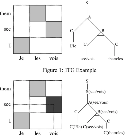
One special case of ITG is the bracketing ITG that has only one nonterminal that instantiates exactly one straight rule and one inverted rule. The ITG we apply in our experiments has more structural labels than the primitive bracketing grammar: it has a start symbolS, a single preterminalC, and two interme-diate nonterminalsAandBused to ensure that only one parse can generate any given word-level align-ment, as discussed by Wu (1997) and Zens and Ney (2003).

As an example, Figure 1 shows the alignment and the corresponding parse tree for the sentence pair Je les vois / I see them using the unambiguous bracket-ing ITG.

A stochastic ITG can be thought of as a stochastic CFG extended to the space of bitext. The indepen-dence assumptions typifying S-CFGs are also valid for S-ITGs. Therefore, the probability of an S-ITG parse is calculated as the product of the probabili-ties of all the instances of rules in the parse tree. For instance, the probability of the parse in Figure 1 is:

P(S→A)·P(A→[CB])

·P(B → hCCi)·P(C→I/Je)

·P(C →see/vois)·P(C→them/les)

It is important to note that besides the bottom-level word-pairing rules, the other rules are all non-lexical, which means the structural alignment com-ponent of the model is not sensitive to the lexical contents of subtrees. Although the ITG model can effectively restrict the space of alignment to make polynomial time parsing algorithms possible, the preference for inverted or straight rules only pas-sively reflect the need of bottom level word align-ment. We are interested in investigating how much help it would be if we strengthen the structural align-ment component by making the orientation choices dependent on the real lexical pairs that are passed up from the bottom.

The first step of lexicalization is to associate a lex-ical pair with each nonterminal. The head word pair generation rules are designed for this purpose:

X →X(e/f)

The word paire/f is representative of the lexical content ofXin the two languages.

For binary rules, the mechanism of head selection is introduced. Now there are 4 forms of binary rules:

X(e/f)→[Y(e/f)Z]

X(e/f)→[Y Z(e/f)]

X(e/f)→ hY(e/f)Zi

X(e/f)→ hY Z(e/f)i

determined by the four possible combinations of head selections (Y orZ) and orientation selections (straight or inverted).

The rules for generating lexical pairs at the leaves of the tree are now predetermined:

X(e/f)→e/f

Putting them all together, we are able to derive a lexicalized bilingual parse tree for a given sentence pair. In Figure 2, the example in Figure 1 is revisited. The probability of the lexicalized parse is:

P(S→S(see/vois))

·P(S(see/vois)→A(see/vois))

·P(A(see/vois)→[CB(see/vois)])

I see them

Je les vois

C B

C A

see/vois them/les I/Je

S

C

Figure 1: ITG Example

I see them

Je les vois

S(see/vois)

C(see/vois) C(I/Je)

C S

C(them/les) C B(see/vois) A(see/vois)

Figure 2: Lexicalized ITG Example. see/vois is the headword of both the 2x2 cell and the entire alignment.

·P(B(see/vois)→ hC(see/vois)Ci)

·P(C→C(them/les))

The factors of the product are ordered to show the generative process of the most probable parse. Starting from the start symbol S, we first choose the head word pair for S, which is see/vois in the example. Then, we recursively expand the lexical-ized head constituents using the lexicallexical-ized struc-tural rules. Since we are only lexicalizing rather than bilexicalizing the rules, the non-head constituents need to be lexicalized using head generation rules so that the top-down generation process can proceed in all branches. By doing so, word pairs can appear at all levels of the final parse tree in contrast with the unlexicalized parse tree in which the word pairs are generated only at the bottom.

The binary rules are lexicalized rather than bilexi-calized.1 This is a trade-off between complexity and expressiveness. After our lexicalization, the number of lexical rules, thus the number of parameters in the statistical model, is still at the order ofO(|V||T|), where |V| and |T| are the vocabulary sizes of the

1_{In a sense our rules are bilexicalized in that they condition}

on words from both languages; however they do not capture head-modifier relations within a language.

two languages.

2.1 Parsing

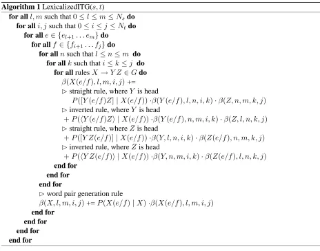
Given a bilingual sentence pair, a synchronous parse can be built using a two-dimensional extension of chart parsing, where chart items are indexed by their nonterminalX, head word paire/fif specified, be-ginning and ending positionsl, min the source lan-guage string, and beginning and ending positionsi, j in the target language string. For Expectation Max-imization training, we compute lexicalized inside probabilities β(X(e/f), l, m, i, j), as well as un-lexicalized inside probabilitiesβ(X, l, m, i, j), from the bottom up as outlined in Algorithm 1.

The algorithm has a complexity of O(Ns4Nt4), whereNsandNtare the lengths of source and tar-get sentences respectively. The complexity of pars-ing for an unlexicalized ITG isO(N3

sNt3). Lexical-ization introduces an additional factor ofO(NsNt), caused by the choice of headwords eand f in the pseudocode.

Algorithm 1 LexicalizedITG(s, t)

for alll, msuch that0≤l≤m≤Nsdo for alli, jsuch that0≤i≤j≤Ntdo

for alle∈ {el+1. . . em}do for allf ∈ {fi+1. . . fj}do

for allnsuch thatl≤n≤m do for allksuch thati≤k≤j do

for all rulesX →Y Z ∈Gdo

β(X(e/f), l, m, i, j)+=

_{straight rule, where}Y _{is head}

P([Y(e/f)Z]|X(e/f))·β(Y(e/f), l, n, i, k)·β(Z, n, m, k, j)

inverted rule, whereY is head

+P(hY(e/f)Zi |X(e/f))·β(Y(e/f), n, m, i, k)·β(Z, l, n, k, j)

_{straight rule, where}Z_{is head}

+P([Y Z(e/f)]|X(e/f))·β(Y, l, n, i, k)·β(Z(e/f), n, m, k, j)

_{inverted rule, where}Z _{is head}

+P(hY Z(e/f)i |X(e/f))·β(Y, n, m, i, k)·β(Z(e/f), l, n, k, j) end for

end for end for

word pair generation rule

β(X, l, m, i, j)+=P(X(e/f)|X)·β(X(e/f), l, m, i, j) end for

end for end for end for

2.2 Pruning

We need to further restrict the space of alignments spanned by the source and target strings to make the algorithm feasible. Our technique involves comput-ing an estimate of how likely each of then4_{cells in}

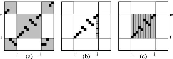
the chart is before considering all ways of building the cell by combining smaller subcells. Our figure of merit for a cell involves an estimate of both the inside probability of the cell (how likely the words within the box in both dimensions are to align) and the outside probability (how likely the words out-side the box in both dimensions are to align). In including an estimate of the outside probability, our technique is related to A* methods for monolingual parsing (Klein and Manning, 2003), although our estimate is not guaranteed to be lower than com-plete outside probabity assigned by ITG. Figure 3(a) displays the tic-tac-toe pattern for the inside and outside components of a particular cell. We use IBM Model 1 as our estimate of both the inside and

outside probabilities. In the Model 1 estimate of the outside probability, source and target words can align using any combination of points from the four outside corners of the tic-tac-toe pattern. Thus in Figure 3(a), there is one solid cell (corresponding to the Model 1 Viterbi alignment) in each column, falling either in the upper or lower outside shaded corner. This can be also be thought of as squeezing together the four outside corners, creating a new cell whose probability is estimated using IBM Model 1. Mathematically, our figure of merit for the cell

(l, m, i, j)is a product of the inside Model 1 proba-bility and the outside Model 1 probaproba-bility:

P(f_(i,j)|e_(l,m))·P(f

(i,j)|e(l,m)) (1)

=λ_|(l,m)|,|(i,j)|

Y

t∈(i,j) X

s∈{0,(l,m)}

t(ft|es)

·λ_{|(l,m)|,|(i,j)|} Y t∈(i,j)

X

s∈{0,(l,m)}

l m

i j i j

l m

i j

(a) (b) (c)

Figure 3: The tic-tac-toe figure of merit used for pruning bitext cells. The shaded regions in (a) show alignments included in the figure of merit for bitext cell(l, m, i, j)(Equation 1); solid black cells show the Model 1 Viterbi alignment within the shaded area. (b) shows how to compute the inside probability of a unit-width cell by combining basic cells (Equation 2), and (c) shows how to compute the inside probability of any cell by combining unit-width cells (Equation 3).

where(l, m)and(i, j)represent the complementary spans in the two languages.λL1,L2 is the probability

of any word alignment template for a pair of L1

-word source string andL2-word target string, which

we model as a uniform distribution of word-for-word alignment patterns after a Poisson distribution of target string’s possible lengths, following Brown et al. (1993). As an alternative, thePoperator can be replaced by themaxoperator as the inside opera-tor over the translation probabilities above, meaning that we use the Model 1 Viterbi probability as our estimate, rather than the total Model 1 probability.2

A na¨ıve implementation would take O(n6)steps of computation, because there areO(n4_{)cells, each}

of which takesO(n2)steps to compute its Model 1 probability. Fortunately, we can exploit the recur-sive nature of the cells. Let INS(l, m, i, j) denote the major factor of our Model 1 estimate of a cell’s inside probability,Q_t∈(i,j)P_{s∈{0,(l,m)}}t(ft|es). It turns out that one can compute cells of width one (i = j) in constant time from a cell of equal width and lower height:

INS(l, m, j, j) = Y

t∈(j,j) X

s∈{0,(l,m)}

t(ft|es)

= X

s∈{0,(l,m)}

t(fj |es)

= INS(l, m−1, j, j)

+t(fj |em) (2)

Similarly, one can compute cells of width greater than one by combining a cell of one smaller width

2_{The experimental difference of the two alternatives was}

small. For our results, we used themaxversion.

with a cell of width one:

INS(l, m, i, j) = Y

t∈(i,j) X

s∈{0,(l,m)}

t(ft|es)

= Y

t∈(i,j)

INS(l, m, t, t)

= INS(l, m, i, j−1)

·INS(l, m, j, j) (3)

Figure 3(b) and (c) illustrate the inductive compu-tation indicated by the two equations. Each of the O(n4) inductive steps takes one additive or mul-tiplicative computation. A similar dynammic pro-graming technique can be used to efficiently com-pute the outside component of the figure of merit. Hence, the algorithm takes justO(n4)steps to com-pute the figure of merit for all cells in the chart.

Once the cells have been scored, there can be many ways of pruning. In our experiments, we ap-plied beam ratio pruning to each individual bucket of cells sharing a common source substring. We prune cells whose probability is lower than a fixed ratio be-low the best cell for the same source substring. As a result, at least one cell will be kept for each source substring. We safely pruned more than 70% of cells using10−5 as the beam ratio for sentences up to 25 words. Note that this pruning technique is applica-ble to both the lexicalized ITG and the conventional ITG.

chart has increased to O(N_s3N_t3) from O(N_s2N_t2)

due to the choice one of O(Ns) source language words and one of O(Nt) target language words as the head. We keep only the top-klexicalized items for a given chart cell of a certain nonterminalY con-tained in the celll, m, i, j. Thus the additional com-plexity of O(NsNt) will be replaced by a constant factor.

The two pruning techniques can work for both the computation of expected counts during the training process and for the Viterbi-style algorithm for ex-tracting the most probable parse after training. How-ever, if we initialize EM from a uniform distribution, all probabilties are equal on the first iteration, giving us no basis to make pruning decisions. So, in our experiments, we initialize the head generation prob-abilities of the formP(X(e/f)|X)to be the same asP(e/f | C) from the result of the unlexicalized ITG training.

2.3 Smoothing

Even though we have controlled the number of pa-rameters of the model to be at the magnitude of O(|V||T|), the problem of data sparseness still ren-ders a smoothing method necessary. We use back-ing off smoothback-ing as the solution. The probabilities of the unary head generation rules are in the form of P(X(e/f) | X). We simply back them off to the uniform distribution. The probabilities of the binary rules, which are conditioned on lexicalized nonter-minals, however, need to be backed off to the prob-abilities of generalized rules in the following forms:

P([Y(∗)Z]|X(∗))

P([Y Z(∗)]|X(∗))

P(hY(∗)Zi |X(∗))

P(hY Z(∗)i |X(∗))

where∗stands for any lexical pair. For instance,

P([Y(e/f)Z]|X(e/f)) =

(1−λ)PEM([Y(e/f)Z]|X(e/f))

+λP([Y(∗)Z]|X(∗))

where

λ= 1/(1 +Expected Counts(X(e/f)))

The more oftenX(e/f)occurred, the more reli-able are the estimated conditional probabilities with the condition part beingX(e/f).

3 Experiments

We trained both the unlexicalized and the lexical-ized ITGs on a parallel corpus of Chinese-English newswire text. The Chinese data were automati-cally segmented into tokens, and English capitaliza-tion was retained. We replaced words occurring only once with an unknown word token, resulting in a Chinese vocabulary of 23,783 words and an English vocabulary of 27,075 words.

In the first experiment, we restricted ourselves to sentences of no more than 15 words in either lan-guage, resulting in a training corpus of 6,984 sen-tence pairs with a total of 66,681 Chinese words and 74,651 English words. In this experiment, we didn’t apply the pruning techniques for the lexicalized ITG. In the second experiment, we enabled the pruning techniques for the LITG with the beam ratio for the tic-tac-toe pruning as10−5and the numberkfor the top-kpruning as 25. We ran the experiments on sen-tences up to 25 words long in both languages. The resulting training corpus had 18,773 sentence pairs with a total of 276,113 Chinese words and 315,415 English words.

We evaluate our translation models in terms of agreement with human-annotated word-level align-ments between the sentence pairs. For scoring the Viterbi alignments of each system against gold-standard annotated alignments, we use the alignment error rate (AER) of Och and Ney (2000), which mea-sures agreement at the level of pairs of words:

AER_{= 1−} |A∩GP|+|A∩GS|

|A|+|GS|

where A is the set of word pairs aligned by the automatic system, GS is the set marked in the gold standard as “sure”, andGP is the set marked as “possible” (including the “sure” pairs). In our Chinese-English data, only one type of alignment was marked, meaning thatGP =GS.

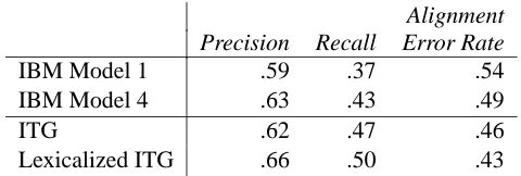
Alignment Precision Recall Error Rate

IBM Model 1 .59 .37 .54

IBM Model 4 .63 .43 .49

ITG .62 .47 .46

Lexicalized ITG .66 .50 .43

Table 1: Alignment results on Chinese-English corpus (≤15 words on both sides). Full ITG vs. Full LITG

Alignment Precision Recall Error Rate

IBM Model 1 .56 .42 .52

IBM Model 4 .67 .43 .47

ITG .68 .52 .40

Lexicalized ITG .69 .51 .41

Table 2: Alignment results on Chinese-English corpus (≤25 words on both sides). Full ITG vs. Pruned LITG

LITG against the unlexicalized ITG.

A separate development set of hand-aligned sen-tence pairs was used to control overfitting. The sub-set of up to 15 words in both languages was used for cross-validating in the first experiment. The subset of up to 25 words in both languages was used for the same purpose in the second experiment.

Table 1 compares results using the full (unpruned) model of unlexicalized ITG with the full model of lexicalized ITG.

The two models were initialized from uniform distributions for all rules and were trained until AER began to rise on our held-out cross-validation data, which turned out to be 4 iterations for ITG and 3 iterations for LITG.

The results from the second experiment are shown in Table 2. The performance of the full model of un-lexicalized ITG is compared with the pruned model of lexicalized ITG using more training data and eval-uation data.

Under the same check condition, we trained ITG for 3 iterations and the pruned LITG for 1 iteration.

For comparison, we also included the results from IBM Model 1 and Model 4. The numbers of itera-tions for the training of the IBM models were cho-sen to be the turning points of AER changing on the cross-validation data.

4 Discussion

As shown by the numbers in Table 1, the full lexical-ized model produced promising alignment results on sentence pairs that have no more than 15 words on both sides. However, due to its prohibitiveO(n8₎

of parameters, leading to a form of overfitting. In contrast, overfitting did not seem to be a problem for LITG in the unpruned experiment of Table 1, despite the much larger number of parameters for LITG than for ITG and the smaller training set.

We also want to point out that for a pair of long sentences, it would be hard to reflect the inherent bilingual syntactic structure using the lexicalized bi-nary bracketing parse tree. In Figure 2,A(see/vois)

echoes IP(see/vois) and B(see/vois) echoes V P(see/vois)so that it meansIP(see/vois)is not inverted from English to French but its right child V P(see/vois)is inverted. However, for longer sen-tences with more than 5 levels of bracketing and the same lexicalized nonterminal repeatedly appearing at different levels, the correspondences would be-come less linguistically plausible. We think the lim-itations of the bracketing grammar are another rea-son for not being able to improve the AER of longer sentence pairs after lexicalization.

The space of alignments that is to be considered by LITG is exactly the space considered by ITG since the structural rules shared by them define the alignment space. The lexicalized ITG is designed to be more sensitive to the lexical influence on the choices of inversions so that it can find better align-ments. Wu (1997) demonstrated that for pairs of sentences that are less than 16 words, the ITG align-ment space has a good coverage over all possibili-ties. Hence, it’s reasonable to see a better chance of improving the alignment result for sentences less than 16 words.

5 Conclusion

We presented the formal description of a Stochastic Lexicalized Inversion Transduction Grammar with its EM training procedure, and proposed specially designed pruning and smoothing techniques. The experiments on a parallel corpus of Chinese and En-glish showed that lexicalization helped for aligning sentences of up to 15 words on both sides. The prun-ing and the limitations of the bracketprun-ing grammar may be the reasons that the result on sentences of up to 25 words on both sides is not better than that of the unlexicalized ITG.

Acknowledgments We are very grateful to Re-becca Hwa for assistance with the Chinese-English

data, to Kevin Knight and Daniel Marcu for their feedback, and to the authors of GIZA. This work was partially supported by NSF ITR IIS-09325646 and NSF ITR IIS-0428020.

References

Hiyan Alshawi, Srinivas Bangalore, and Shona Douglas. 2000. Learning dependency translation models as col-lections of finite state head transducers. Computa-tional Linguistics, 26(1):45–60.

Adam Berger, Peter Brown, Stephen Della Pietra, Vin-cent Della Pietra, J. R. Fillett, Andrew Kehler, and Robert Mercer. 1996. Language translation apparatus and method of using context-based tanslation models. United States patent 5,510,981.

Peter F. Brown, Stephen A. Della Pietra, Vincent J. Della Pietra, and Robert L. Mercer. 1993. The mathematics of statistical machine translation: Parameter estima-tion. Computational Linguistics, 19(2):263–311.

Dan Klein and Christopher D. Manning. 2003. A* pars-ing: Fast exact viterbi parse selection. In

Proceed-ings of the 2003 Meeting of the North American chap-ter of the Association for Computational Linguistics (NAACL-03).

I. Dan Melamed. 2003. Multitext grammars and syn-chronous parsers. In Proceedings of the 2003 Meeting

of the North American chapter of the Association for Computational Linguistics (NAACL-03), Edmonton.

Franz Josef Och and Hermann Ney. 2000. Improved statistical alignment models. In Proceedings of the

38th Annual Conference of the Association for Compu-tational Linguistics (ACL-00), pages 440–447, Hong

Kong, October.

Dekai Wu. 1997. Stochastic inversion transduction grammars and bilingual parsing of parallel corpora.

Computational Linguistics, 23(3):377–403.

Kenji Yamada and Kevin Knight. 2001. A syntax-based statistical translation model. In Proceedings of the

39th Annual Conference of the Association for Com-putational Linguistics (ACL-01), Toulouse, France.

Richard Zens and Hermann Ney. 2003. A comparative study on reordering constraints in statistical machine translation. In Proceedings of the 40th Annual

Meet-ing of the Association for Computational LMeet-inguistics,

Sapporo, Japan.

Hao Zhang and Daniel Gildea. 2004. Syntax-based alignment: Supervised or unsupervised? In

Proceed-ings of the 20th International Conference on Compu-tational Linguistics (COLING-04), Geneva,