Munich Personal RePEc Archive
The cost of travel time variability: three
measures with properties
Engelson, Leonid and Fosgerau, Mogens
Royal Institute of Technology, Sweden, Danish Technical University
2016
Online at
https://mpra.ub.uni-muenchen.de/72255/
1
The cost of travel time variability: three measures with properties
1Leonid Engelson2, Mogens Fosgerau3
Abstract
This paper explores the relationships between three types of measures of the cost of travel time variability: measures based on scheduling preferences and implicit departure time choice, Bernoulli type measures based on a univariate function of travel time, and dispersion measures. We characterise measures that are both scheduling measures and mean-dispersion measures and measures that are both Bernoulli and mean-mean-dispersion. There are no measures that are both scheduling and Bernoulli. We consider the impact of requiring that measures are additive or homogeneous, proving also a new strong result on the utility rates in an additive scheduling measure. These insights are useful for selecting cost measures to use in applications.
Keywords: value; travel time; variability; reliability
Highlights:
• Considers three types of measures of the cost of travel time variability
• Includes probably all cost measures ever used
• Clarifies the relations between these types and the restrictions embodied in each
• Clarifies restriction implied by requiring additivity or homogeneity
• Useful for choosing cost measures for applications
1. Introduction
This paper considers three types of measures of the cost to travellers of travel time variability that have been used in travel demand modelling and transportation economics. We consider measures based on scheduling preferences, Bernoulli type measures based on a univariate cost function, and mean-dispersion measures. The objective of the paper is to decide to which extent such measures are the same. That is, when can a measure of one type be represented as a measure of another type? This is important, as it informs the modelling choice of which cost measure to use in a given context, depending on which properties that one desires for a cost measure. We introduce the different measures in detail below.
Travel time variability, the fact that travel times are random and unpredictable from the point of view of travellers, is an important problem in general. Traffic congestion not only induces delays, but also makes travel times highly variable and unpredictable. The economic cost to
1
We thank the editor and the referees for their comments which have helped us improve the paper. Fosgerau is supported by the Danish Innovation Fund. Engelson is supported by the Center for Transport Studies at KTH.
2
KTH Royal Institute of Technology, Sweden. [email protected]
3
2
societies of travel time variability is comparable to the cost of average delays and is therefore clearly significant from the perspective of national economies (see e.g. Winston 2013 for an overview). It is therefore of interest to first be able to describe how travellers behave when faced with travel time variability and second to be able to take the effect on travel time variability into account when we evaluate alternative transport policy measures, infrastructure investments or other interventions in the transport system. It is also important to be able to communicate the extent of travel time variability to the public. For these purposes we require measures of the cost to travellers of travel time variability. Cost measures may have advantages in terms of communication to the public, they may have advantages in terms of mathematical simplicity, or they may have advantages in terms of their foundation in underlying theory. Most importantly, of course, they may differ in their ability to describe observed behaviour. We define some useful properties that cost measures may have and show how these properties constrain which types of cost measures are possible. This is informative about how different advantages may be combined in one cost measure.
The first type of measure that we consider is based on scheduling preferences. We consider forms in which travellers achieve utility at some rate prior to departure and at some other rate upon arrival at the destination of a trip. Then the utility cost of a trip depends on the departure time and on the arrival time and thereby indirectly on the random duration of the trip. The departure time is assumed to be chosen such that it maximises the expected utility. The main advantage of scheduling measures is that they have a foundation in an underlying theory of scheduling behaviour. This ensures basically that scheduling measures make behavioural sense, being consistent with a description of rational scheduling behaviour. Furthermore, the underlying scheduling model may be used to predict departure times.
The second type of measures is inspired by the economics literature on risk preferences going back to Bernoulli (1954, translated from the 1738 original), which considers utility as a function of a monetary amount. It is possible instead to consider the time-related utility cost of a trip to be just a function of travel time with the timing of the trip playing no role. When travel time is random, travellers are assumed to care about the expected utility cost. An advantage of this type of measure is that it makes it possible to employ the corresponding economic theory regarding risk preferences. We ask among other things whether a Bernoulli type cost measure is consistent with the existence of underlying scheduling preferences and find that the answer to this question is negative in general.
The third type of measures consists of measures that are linear in the mean travel time and some measure of the dispersion of travel time. These measures are then defined directly in terms of statistics of the travel time distribution, not relying on an underlying classical utility defined over travel outcomes. This type of measure has the advantage that it can build on some concept of travel time variability that is deemed to be intuitive and capable of being widely communicated. Mean-dispersion models include the mean-standard deviation model, the mean-variance model as well as models that take the expected time cost to depend on the mean and the difference between two quantiles of the travel time distribution. We find that a mean-dispersion measure is equal to a Bernoulli measure only if the measure is proportional to the mean travel time while the travel time variability plays no role.
3
sum of the cost measure applied to the two components. Additivity is useful in network models for aggregating costs from the link level to the path level, when one is prepared to assume that travel times are (sufficiently) independent across links. We find that all additive scheduling measures are also dispersion measures, while there exists additive mean-dispersion measures that are not scheduling measures.
A cost measure is homogeneous if multiplying travel time by a positive factor scales the cost by the same factor. This is a useful property, since it implies that a change in the time unit only affects the scale of the cost measure. It is furthermore useful in relation to mean-dispersion measures: we may define the reliability ratio to be the ratio between the marginal cost of dispersion to the marginal cost of mean travel. Homogeneity then implies that the reliability ratio is independent of the scale of the travel time distribution. Most mean-dispersion measures used in practice have this property. We find, however, that there are no homogeneous cost measures that are both mean-dispersion measures and scheduling measures. Thus, requiring homogeneity of a mean-dispersion measure rules out that it can have a foundation in a scheduling model. We also find that any homogeneous Bernoulli measure must be proportional to the mean travel time and hence it is not sensitive to random travel time variability.
The scientific literature on travel time variability is becoming large. We provide some bibliographical notes at the end of each the three sections introducing the different cost measures. More generally, a recent introduction is Fosgerau (2015). Recent literature reviews are provided in Carrion and Levinson (2012) and Li et al. (2010). Small (2012) reviews the broader literature on the valuation of travel time. Concerning freight transport, a recent review is provided by Feo-Valero et al. (2011). The reader may refer to these papers for a more comprehensive overview of the literature.
The layout of the paper is the following. Section 2 introduces the three types of measures, along with references to the literature. Section 3 presents our results concerning equivalence of cost measures, Section 4 considers additivity and homogeneity, while Section 5 concludes. 2. Three types of travel time cost measures
Travel time 𝑇 ≥0 is a bounded, almost surely non-negative random variable, and the class of all these random variables is denoted Φ. This includes, e.g., all non-negative discrete distributions. The assumption that travel time is bounded ensures that all relevant integrals will exist, which is convenient for the mathematical exposition. This does not prevent the cost measures that we will consider being applied to unbounded distributions, such as the normal, lognormal, gamma and stable distributions that have been applied in the literature.
In general, a travel time cost measure is a functional C:Φ → ℝ, In this section we will define the three types that we discuss in this paper. For the sake of brevity, we shall talk just about cost measures.
2.1. Type 1: scheduling preference based cost measures
4
achieved at the destination at time 𝑠 after the completion of the trip. The utility rate during the trip is normalised to zero, such that the utility rates ℎ,𝑤 may be understood as differences from the utility rate achieved while travelling.
Assume further that ℎ,𝑤 are differentiable with ℎ′(𝑠)≤ 0 <𝑤′(𝑠) for all 𝑠 and that ℎ(0) =
𝑤(0) and with 𝑤′ being continuous. These assumptions guarantee that the traveller prefers to be at the origin prior to time 0 and prefers to be at the destination after time 0. The location of the intersection of ℎ and 𝑤 at time 0 is a normalisation causing no loss of generality. Denote for convenience the primitive functions 𝐻(𝑠) =∫ ℎ𝐾𝑠 (𝑟)𝑑𝑟
1 and 𝑊(𝑠) =∫ 𝑤(𝑟)𝑑𝑟
𝑠
𝐾2 for some
constants 𝐾1,𝐾2.
The traveller incurs utility 𝐻(𝑡𝑑)− 𝑊(𝑡𝑎), where 𝑡𝑑 is the departure time, and 𝑡𝑎 is the arrival time. This embodies then the restriction that utility is separable into a component that depends on the departure time and a component that depends on the arrival time. The constants 𝐾1,𝐾2 are set equal to zero; this changes utility by a constant, which has no consequences for the implied preferences.
The arrival time is random and is given in terms of the departure time and the random travel time by 𝑡𝑑+𝑇=𝑡𝑎.
The traveller chooses departure time to maximise the expected utility 𝐻(𝑡𝑑)− 𝐸𝑊(𝑡𝑑+𝑇). This problem is equivalent to minimisation of the expected utility cost
𝐶1[𝑇] = min𝑡
𝑑 [𝐸𝑊(𝑡𝑑+𝑇)− 𝐻(𝑡𝑑)]. (1)
The first-order condition for (1) is 𝐸𝑤(𝑡𝑑+𝑇)− ℎ(𝑡𝑑) = 0. The left hand side of the first-order condition is increasing in 𝑡𝑑, which implies that the optimal departure time is unique. Substituting the optimal departure time into (1) yields the scheduling cost measure.
The first-order condition depends on 𝑇, which shows that the distribution of travel time affects the scheduling cost measure in two ways: directly through 𝑇 in 𝐸𝑊(𝑡𝑑 +𝑇) and indirectly through the choice of departure time 𝑡𝑑. In the Bernoulli measure discussed below, the travel time distribution has only the direct effect as there is no departure time in that measure.
2.1.1. Bibliographical notes
A limiting case of the general scheduling model discussed here is the well-known step model based on 𝛼 − 𝛽 − 𝛾 preferences (Vickrey 1973; K. Small 1982).In this model, the utility rate at the origin is a constant ℎ(𝑠) =𝛼, while the utility rate at the destination is a step function
𝑤(𝑠) = (𝛼 − 𝛽) + 1{𝑠≥0}(𝛽+𝛾), where 𝛽< 𝛼< 𝛽+𝛾.This is not differentiable and does then not fit into the framework for scheduling cost measures that we discuss in this paper.The minimisation problem (1) can be solved with these utility rates for any travel time distribution, leading to a cost measure which is
𝐶[𝑇] =𝛼𝐸𝑇+𝜎(𝛽+𝛾)� 𝐹−1(𝑠)𝑑𝑠 1
𝛾 𝛽+𝛾
5
where 𝜎 is the standard deviation of travel time and 𝐹 is the cumulative distribution function of standardised travel time (Noland and Small 1995; Bates et al. 2001; Fosgerau and Karlstrom 2010). We note that the marginal cost of standard deviation depends on the standardized distribution of travel time, but that it is constant if the standardized distribution of travel time is fixed.
The time-varying utility rate formulation in terms of ℎ,𝑤 is originally due to Vickrey (1973) and was revived by Tseng and Verhoef (2008). The use of this model to value travel time variability is due to Fosgerau and Engelson (2011) who used linear utility rates to find a cost measure that is linear in the mean and variance of the travel time distribution when ℎ is constant. In this case, the cost measure is additive over independent travel time components, and the additivity property was characterized in Engelson and Fosgerau (2011). Engelson (2011) explored exponential and quadratic utility rates. These models have been applied empirically in, e.g., Börjesson, Eliasson, and Franklin (2012), Hjorth et al. (2015), and Abegaz, Hjorth, and Rich (2015).
The micro-economic theory on the value of travel time begins with Becker (1965). Johnson (1966) introduced work time and Oort (1969) introduced travel time into the framework. Oort introduced the interpretation that the utility rates ℎ,𝑤 may be understood as the difference between the utility rate achieved at the origin or the destination and the utility rate achieved during travelling.
2.2. Type 2: Bernoulli cost measures
In this type of model the time cost is calculated based on the time cost function 𝑐 with the properties 𝑐(0) = 0 and 𝑐′> 0. The expected cost is obtained simply as
𝐶2[𝑇] =𝐸𝑐(𝑇). (2) 2.2.1. Bibliographical notes
This model originates from Bernoulli (1954) and was used in a transportation, e.g., by de Palma and Picard (2005), and Cominetti and Torrico (2013). There is a large economic literature on risk preferences (see e.g. Mas-Colell, Whinston, and Green 1995) where there is a utility function instead of the current cost function 𝑐. The risk-preferences of the traveller are captured by the curvature of 𝑐, with convexity of 𝑐 implying risk aversion. Specific functional forms are associated with constant absolute or relative risk aversion.
When only the route choice is considered, i.e. when the departure time is fixed, the scheduling model reduces to 𝐶1[𝑇] =𝐸𝑊(𝑡𝑑+𝑇) which is equivalent to (2) with 𝑐(𝑇) =𝑊(𝑡𝑑+𝑇). A question is, however, if this formulation can be used to study how changes in the travel time variability affect travel cost from a user perspective. Indeed, to cope with travel time uncertainty the traveller may not only modify the route but also adjust the departure time, for example allow a margin for possibly longer travel time. The cost of travel time uncertainty will be overestimated in general if this behaviour is not taken into account.
2.3. Type 3: mean-dispersion models
6
in CBA. Let Ω:Φ → ℝ that satisfies Ω[𝑇] = 0 if and only if 𝑇 is degenerate and is positive otherwise. We also require that
∀𝜎> 0:𝜕Ω[𝜎𝑇]
𝜕𝜎 > 0,
(3)
whenever 𝑇 is a non-degenerate random variable. This assumption ensures that these measures are indeed sensitive to dispersion. We require further that Ω is independent of the location of the random travel time, i.e. Ω[𝑇+𝑏] =Ω[𝑇] for all 𝑏 ∈ ℝ. Then we define
𝐶3[𝑇] =𝛿1𝐸𝑇+𝛿2Ω[𝑇]. (4)
2.3.1. Bibliographical notes
Fosgerau and Karlstrom (2010) showed that the cost measure derived from a scheduling model with the function ℎ being constant and the function 𝑤 being a step function respectively reduces to a mean-standard deviation measure if the standardised travel time distribution 𝐹 is fixed. This is not a mean-dispersion measure in the sense considered here where we do not impose the assumption that the standardised travel time distribution is fixed. Small, Winston and Yan (2005), for example, measured travel time variability by the difference between the 80% quantile and the median of travel time. Such measures have the empirical advantage of being fairly robust, where other measures may be more sensitive to extreme travel times in the tail of the travel time distribution. This may explain why Small, Winston and Yan (2005) found their measure of travel time variability to fit their data better than the standard deviation of travel time. Other studies have used the buffer time index, defined as the difference between, e.g., the 95% quantile of the travel time distribution and the mean travel time.
If we restrict attention to absolutely continuous travel time distributions, then the family of mean-dispersion measures includes all measures based on the difference between two quantiles of the travel time distribution. Letting 𝐹(𝑡) =𝑃(𝑇 ≤ 𝑡) be a cumulative travel time distribution, and 0 <𝑞1 < 𝑞2 < 1, we may let Ω[T] =𝐹−1(𝑞2)− 𝐹−1(𝑞1). Then, for 𝜎> 0, the random travel time 𝜎𝑇 satisfies Ω[𝜎𝑇] =𝜎Ω[𝑇], which makes it clear that 𝐶3, with Ω specified in this way, is a mean-dispersion measure according to the definition given here. The reason why we need to restrict attention to absolutely continuous travel time distributions is that we need to avoid the situation where 𝐹−1(𝑞2)− 𝐹−1(𝑞1) = 0, which would violate the condition in (3).
The family of mean-dispersion measures includes also the buffer time, if we again consider only absolutely continuous travel time distributions. Define Ω[𝑇] =𝐹−1(𝑞)− 𝐸𝑇, where 𝑞 is, e.g., 0.95. Then Ω[𝜎𝑇] =𝜎Ω[𝑇]. The buffer time index (Lyman and Bertini 2008) is intended to describe reliability at the network level and it is not a cost measure in the sense considered in this paper, since it is the buffer time divided by the mean travel time, which makes it a relative measure.
7
time, which would be the buffer time, since the mean travel time enters the cost measure separately.
Fosgerau and Engelson (2011) showed that a scheduling model with constant ℎ and affine 𝑤 leads to a mean-variance cost measure, where the coefficients 𝛿1 and 𝛿2 do not depend on the travel time distribution. Then the utility rates considered by Fosgerau and Engelson (2011) lead to a mean-dispersion measure of the kind considered in this paper.
3. Equivalence results
Define 𝒞1 to be the class of scheduling measures 𝐶1, 𝒞2 to be the class of Bernoulli measures
𝐶2, and 𝒞3 to be the class of mean-dispersion measures 𝐶3.
We say that two cost measures are equal if they coincide for all random travel time variables. We further say that two classes of measures are equivalent if for any member of one class there is an equal member of the second and vice versa.
Our first theorem states that the class of scheduling measures does not overlap with the class of Bernoulli measures. In other words, there is no scheduling measure that is a Bernoulli measure, and there is no Bernoulli measure that is a scheduling measure.
Theorem 1. A scheduling measure and a Bernoulli measure are never equal, i.e. 𝒞1∩ 𝒞2 = ∅. Proof. Let 𝐶1 be a scheduling measure based on utility rates ℎ and 𝑤, and let 𝐶2 be a Bernoulli measure based on the function 𝑐, satisfying the conditions stated in the previous section. Assume, seeking a contradiction, that
𝐶1[𝑇] =𝐶2[𝑇] for any 𝑇 ∈ Φ. (5) Then for fixed non-negative travel time 𝑡 (a unit mass at 𝑡), we have
min
𝑡𝑑 [𝑊(𝑡𝑑+𝑡)− 𝐻(𝑡𝑑)] =𝑐(𝑡)
(6) from (1) and (2).
Consider now a random travel time 𝑇 taking two values: t with probability 𝑝 and 0 with probability 1− 𝑝. Then from (1) we obtain
𝐶1[𝑇] = min𝑡
𝑑 [(1− 𝑝)𝑊(𝑡𝑑) +𝑝𝑊(𝑡𝑑 +𝑡)− 𝐻(𝑡𝑑)]
(7)
while from (2) we get𝐶2[𝑇] = (1− 𝑝)𝑐(0) +𝑝𝑐(𝑡) =𝑝𝑐(𝑡) and, using (6),
𝐶2[𝑇] =𝑝min𝑡𝑑[𝑊(𝑡𝑑 +𝑡)− 𝐻(𝑡𝑑)]. (8)
It follows from (5) that the right hand sides of (7) and (8) coincide for any 𝑡 and 𝑝. Differentiating both optimal values with respect to 𝑡 and using the envelope theorem yields
8
p𝑤(𝑡1+𝑡)− ℎ(𝑡1) = 0, or (1− 𝑝)[𝑤(𝑡1)− 𝑤(𝑡1+𝑡)] = ℎ(𝑡1)− 𝑤(𝑡1+𝑡). Since the right hand side of the latter equation is independent of 𝑝, this implies that for any nonnegative
𝑡 there is 𝑡1 such that 𝑤(𝑡1) =𝑤(𝑡1+𝑡), which contradicts the assumption that 𝑤′ > 0. ■ The next theorem considers the relationship between Bernoulli measures and mean-dispersion measures. It shows that the only way that a cost measure can belong to both classes is if the cost measure is trivial, depending only on the mean travel time. In other words, a cost measure that does not only depend on the mean travel time cannot both be a Bernoulli measure and a mean-dispersion measure.
Theorem 2. A Bernoulli measure 𝐶2[𝑇] =𝐸𝑐(𝑇) is equal to a mean-dispersion measure
𝐶3[𝑇] =𝛿1𝐸𝑇+𝛿2Ω(𝑇) if and only if 𝑐(𝑡)≡ 𝛿1𝑡 and 𝛿2 = 0.
Proof. Taking travel time as a fixed non-negative number 𝑡 one obtains 𝐶2[𝑡] =𝑐(𝑡) and
𝐶3[𝑡] =𝛿1𝑡, from (2) and (4), hence 𝑐(𝑡) =𝛿1𝑡 for all 𝑡 ≥0. For any non-degenerate random travel time 𝑇 we have by assumption that Ω[𝑇] > 0. From 𝐶2[𝑇] =𝛿1𝐸𝑇, comparison with
(4) yields 𝛿2 = 0. ■
In conclusion, Bernoulli measures have no interesting overlaps with scheduling measures or with mean-dispersion measures. We shall therefore concentrate on the overlap between scheduling measures and mean-dispersion measures. The overlap between these two classes is characterised in the following theorem.
Theorem 3. A scheduling measure is also a mean-dispersion measure if and only if ℎ(𝑠) =𝛿1 for all 𝑠 ≤0.
Proof. Consider a cost measure 𝐶 that is both a scheduling measure and a mean-dispersion measure. Since 𝐶 is a mean-dispersion measure, we have 𝐶[𝑡] =𝛿1𝑡 for all 𝑡 ≥0. Use the envelope theorem on 𝐶[𝑡] to find that 𝑤(𝑡𝑑+𝑡) =𝛿1, which implies that 𝑡𝑑 = −𝑡. Then the first-order condition from the choice of 𝑡𝑑 implies that ℎ(−𝑡) =𝛿1 for all 𝑡 ≥0.
To prove the reverse implication, assume that ℎ(𝑠) =𝛿1 for all 𝑠 ≤0. Let travel time be
𝜇+𝑋 with 𝐸𝑋= 0. We have to show that 𝐶[𝜇+𝑋] =𝛿1𝜇+𝐶[𝑋] for all 𝜇 ≥0. This is true for 𝜇 = 0. The first-order condition for minimizing the scheduling cost is 𝛿1 = 𝐸𝑤(𝑡𝑑+𝜇+
𝑋). Then
𝜕𝐶[𝜇+𝑋]
𝜕𝜇 =𝐸𝑤(𝑡𝑑+𝜇+𝑋) =𝛿1,
and 𝐶 satisfies (4) with 𝛿2 = 1 and Ω[𝑇] = 𝐶[𝑇 − 𝐸𝑇].
Finally, to establish (3), note first that for a non-degenerate random variable 𝑇 and an increasing function 𝑣 we have 𝐸�(𝑇 − 𝐸𝑇)𝑣(𝑇)�> 0.4 Then, if travel time 𝑇 has a non-degenerate distribution,
𝜕C[𝜎𝑇]
𝜕𝜎 =𝛿1𝐸𝑇+
𝜕Ω[𝜎𝑇]
𝜕𝜎 = 𝐸𝑇𝑤(𝑡𝑑+𝜎𝑇)
4
This can be shown by first noting that 𝐸𝑇= 0 and 𝑣(0) = 0 can be assumed at no loss of generality. Then
9
> 𝐸𝑇 ∙ 𝐸𝑤(𝑡𝑑+𝜎𝑇) =𝛿1𝐸𝑇, (9)
where the inequality follows since 𝑤 is increasing and therefore the covariance of 𝑇 and
𝑤(𝑡𝑑 +𝜎𝑇) is positive. Hence
𝜕Ω[𝜎𝑇]
𝜕𝜎 > 0
as required. ■
Theorem 3 establishes that a scheduling measure is also a mean-dispersion measure if and only if the utility rate at home in the scheduling measure is constant until time 0.This leads to the question whether it is true that any mean-dispersion measure can be represented as a scheduling measure. However, the answer to this question is no, according to Theorem 5, below where we will construct a mean-dispersion measure that is not a scheduling measure. 4. Additivity and homogeneity
We now introduce two useful properties that cost measures may have. We denote by 𝒞𝐴 the class of cost measures 𝐶:Φ → ℝ that are additive, i.e. 𝐶[𝑇1+𝑇2] =𝐶[𝑇1] +𝐶[𝑇2], whenever
𝑇1,𝑇2 are independent. We denote by 𝒞𝐻 the class of cost measures 𝐶:Φ → ℝ that are
homogeneous if 𝐶[𝜎𝑇] =𝜎𝐶[𝑇], whenever 𝜎 ≥0.
The following theorem is stronger than the results established in Engelson and Fosgerau (2011). The earlier paper demonstrated first that additivity required ℎ to be constant. It then needed additivity for a range of values of ℎ as well as three times differentiability of 𝑤 to establish that 𝑤 must be exponential. Here we merely require 𝑤 to be continuously differentiable and we do not require a range of values for ℎ.
Theorem 4. A scheduling measure 𝐶 ∈ 𝒞1 is additive if and only if ℎ is constant and either
𝑤(𝑠) =ℎ+𝛾
𝛽�𝑒𝛽𝑠−1� or 𝑤(𝑠) =ℎ+𝛾𝑠 where 𝛾 > 0 and 𝛽 ≠0.
Proof. Engelson and Fosgerau (2011) prove that the scheduling measure 𝐶 is additive when
ℎ,𝑤 are as stated in the theorem. Thus the “if” part of the theorem has already been established.
To prove the “only if” part of the theorem assume now that 𝐶 is additive. Theorem 2 in Engelson and Fosgerau (2011) establishes that then ℎ is constant. We do not repeat this proof here.
Let 𝑇𝑖,𝑖= 1,2 be independent random variables that assume values 𝑡𝑖 > 0 with probability 𝑝 and 0 with probability 1− 𝑝, where 0 < 𝑝< 1. Then by additivity of 𝐶 and independence of
𝑇1,𝑇2, we have 𝐶[𝑇1+𝑇2] =𝐶[𝑇1] +𝐶[𝑇2], where the first term does not depend on 𝑡2 and the second term does not depend on 𝑡1. Therefore
𝜕2𝐶[𝑇1+𝑇2]
𝜕𝑡1𝜕𝑡2 = 0. (10)
Writing out the scheduling cost using (1) yields
𝐶[𝑇1+𝑇2] = min 𝑡𝑑
10
= min
𝑡𝑑 {(1− 𝑝)
2𝑊(𝑡
𝑑) +𝑝(1− 𝑝)𝑊(𝑡𝑑 +𝑡1) +𝑝(1− 𝑝)𝑊(𝑡𝑑+𝑡2) +𝑝2𝑊(𝑡𝑑+𝑡1+𝑡2)
− 𝐻(𝑡𝑑)},
which leads to the first-order condition for the choice of departure time with travel time
𝑇1+𝑇2:
ℎ= (1− 𝑝)2𝑤(𝑡𝑑) +𝑝(1− 𝑝)𝑤(𝑡𝑑+𝑡1) +𝑝(1− 𝑝)𝑤(𝑡𝑑+𝑡2) +
𝑝2𝑤(𝑡
𝑑 +𝑡1 +𝑡2). (11)
This equation defines 𝑡𝑑 as a continuous function of 𝑝, 𝑡1 and 𝑡2 since the left hand side is increasing in 𝑡𝑑 and jointly continuous. Carrying out the differentiation in (10) leads to
0 = 𝑝(1− 𝑝)𝑤′(𝑡𝑑+𝑡1)𝜕𝑡𝑑 𝜕𝑡2+𝑝
2𝑤′(𝑡
𝑑+𝑡1+𝑡2)�1 +𝜕𝑡𝜕𝑡𝑑2�, (12) which can be rewritten (differentiating the first-order condition to find 𝜕𝑡𝑑
𝜕𝑡2) and reduced to
become
𝑤′(𝑡
𝑑)𝑤′(𝑡𝑑+𝑡1+𝑡2) =𝑤′(𝑡𝑑 +𝑡1)𝑤′(𝑡𝑑+𝑡2). (13)
Since 𝑤 is continuously differentiable with 𝑤′> 0, we may define the continuous function
𝑣(𝑡) = ln𝑤′(𝑡)−ln𝛾 where we define 𝛾 =𝑤′(0). Then (13) becomes the linear equation
𝑣(𝑡𝑑) +𝑣(𝑡𝑑+𝑡1+𝑡2) =𝑣(𝑡𝑑+𝑡1) +𝑣(𝑡𝑑+𝑡2). (14)
For 𝑝 = 0, (11) becomes ℎ =𝑤(𝑡𝑑) which implies that 𝑡𝑑 = 0. Similarly, 𝑝= 1 implies that
𝑡𝑑 = −(𝑡1+𝑡2). This shows that as 𝑝 varies from 0 to 1, then 𝑡𝑑 varies continuously from 0 to −(𝑡1+𝑡2), since we have noted that 𝑡𝑑 is a continuous function of 𝑝. For any positive values of 𝑡1 and 𝑡2, we may then determine 𝑝 such that 𝑡𝑑 attains any given value in the interval (−(𝑡1+𝑡2), 0). By continuity, (13) is valid for any 𝑡𝑑 in [−(𝑡1+𝑡2), 0]. In particular, taking into account that 𝑣(0) = 0 and by choosing 𝑡𝑑 = 0,𝑡𝑑 = −(𝑡1+𝑡2), and
𝑡𝑑=−𝑡1 we obtain from (13) the Cauchy equation
𝑣(𝑡+𝑠) =𝑣(𝑡) +𝑣(𝑠), (15)
for 𝑡 and 𝑠 both positive, both negative, and of different signs respectively. Since 𝑣 is continuous it follows from Theorem 2.1.1 in Aczél (1966) that 𝑣(𝑠) =𝛽𝑠 for some real 𝛽. Working backwards, we then find that
𝑤′(𝑠) =𝛾𝑒𝛽𝑠 (16)
for any 𝑠. Then the conclusion follows by integration in the two cases 𝛽 ≠0, 𝛽= 0 and the
11
The next theorem concerns the additivity property in relation to scheduling and mean-dispersion measures. We find that if a scheduling measure is additive, then it is also a mean dispersion measure. Not all additive mean-dispersion measures are scheduling measures, however: additive mean-dispersion measures exist that are not scheduling measures.
Theorem 5. All additive scheduling measures are mean-dispersion measures, but there exists additive mean-dispersion measures that are not scheduling measures: 𝒞1∩ 𝒞𝐴 ⊊ 𝒞3∩ 𝒞𝐴. Proof. From Theorem 4, additive scheduling measures have constant ℎ and 𝑤(𝑠) =ℎ+
𝛾
𝛽�𝑒𝛽𝑠−1� with 𝛽 ≠0, or 𝑤(𝑠) =ℎ+𝛾𝑠. Engelson and Fosgerau (2011) show that then
𝐶1[𝑇] =ℎ𝐸𝑇+𝛽𝛾2ln𝐸𝑒𝛽(𝑇−𝐸𝑇) or 𝐶1[T] =ℎ𝐸𝑇+𝛾𝜎2(𝑇). The proof of this is a
straightforward calculation, using, e.g. in the first case, that the first-order condition for the optimal departure time is 𝑡𝑑 =−1
𝛽ln𝐸𝑒𝛽𝑇. We need to establish (3), but this follows in the first case since 𝜕 ln 𝐸𝑒𝜎𝜎
(𝑇−𝐸𝑇)
𝜕𝜕 =
𝐸�𝛽(𝑇−𝐸𝑇)𝑒𝜎𝜎(𝑇−𝐸𝑇)�
𝐸𝑒𝜎𝜎(𝑇−𝐸𝑇) >
𝐸[(𝑇−𝐸𝑇)]𝐸�𝛽𝑒𝜎𝜎(𝑇−𝐸𝑇)�
𝐸𝑒𝜎𝜎(𝑇−𝐸𝑇) > 0
where the first inequality follows since 𝛽𝑒𝜕𝛽(𝑇−𝐸𝑇) is an increasing function of 𝑇. The second case follows just since 𝑇 is non-degenerate. Then these measures belong also to 𝒞3, which proves the first statement of the theorem.
To prove the second part of the theorem, we shall construct an additive mean-dispersion measure that is not a scheduling measure. Note first that the sum of two additive scheduling measures belongs also to 𝒞3. We shall construct a sum of two specific such measures and assume, to get a contradiction, that the sum also belongs to 𝒞1. We omit the first terms comprising the means at no loss of generality. So in the case with 𝐶1 we assume that there exist 𝛽,𝛾 solving for all 𝑇 ∈ Φ either the equation
𝛾
𝛽2ln𝐸𝑒𝛽(𝑇−𝐸𝑇) = ln𝐸𝑒𝑇−𝐸𝑇+ 1 4ln𝐸𝑒
2(𝑇−𝐸𝑇),
or the equation
𝛾𝜎2(𝑇) = ln𝐸𝑒𝑇−𝐸𝑇 +1 4ln𝐸𝑒
2(𝑇−𝐸𝑇),
where ln𝐸𝑒𝑇−𝐸𝑇+1 4ln𝐸𝑒2
(𝑇−𝐸𝑇) ∈ 𝒞
3. To obtain a contradiction we use a random travel time 𝑇 that takes values 𝑎 and 3𝑎 with probabilities ½. Then in the first case
𝛾
𝛽2ln cosh 𝛽𝑎 −ln cosh 𝑎 − 1
4ln cosh 2𝑎 = 0 (17)
for any positive 𝑎, where cosh 𝑥=𝑒𝑥+𝑒−𝑥
2 . As 𝑎 → ∞, the left hand side of (17) has an asymptote
�𝛽 −𝛾 32� 𝑎 − �𝛽𝛾2−54�ln 2,
which leads to 𝛾 𝛽=
3 2 and
𝛾 𝛽2 =
5
4, and then 𝛽 = 6 5 .
12
5 4∙
36 25∙
1
cosh265𝑎
−cosh12𝑎 −cosh122𝑎= 0.
Insert 𝑎= 0 to get 9
5−1−1 = 0, which is a contradiction. The second case leads to the equation
𝛾𝑎2−ln cosh 𝑎 −1
4ln cosh 2𝑎= 0
for any positive 𝑎. This also implies a contradiction, since the second derivative of the left hand side can be zero at 𝑎 = 0 only with 𝛾 = 1 but this makes the first derivative tend to
infinity as 𝑎 → ∞. ■
We now turn to homogeneous cost measures and find that a homogeneous cost measure cannot both be a scheduling measure and a mean-dispersion measure.
Theorem 6. A scheduling measure is never homogeneous: 𝒞1∩ 𝒞𝐻 = ∅.
Proof. To get a contradiction, we will assume that the scheduling measure 𝐶 ∈ 𝒞1 is homogeneous, i.e. that 𝐶[𝜎𝑇] =𝜎𝐶[𝑇] for all positive 𝜎. Consider travel time that is fixed at
𝑡 such that 𝐶[𝑡] =𝐶(𝑡) is just a real function of 𝑡. Then 𝐶( ) is homogeneous, (𝜎𝑡) =
𝜎𝐶(𝑡) and with 𝑡= 1 we get 𝐶(𝜎) =𝜎𝐶(1) and hence 𝐶′(𝑡) =𝐶(1). From the scheduling definition of 𝐶, using enveloping, we get
𝐶(1) = 𝑤(𝑡+𝑡𝑑). (18)
Then, using the same argument as in the proof of Theorem 3, it follows that ℎ(𝑠) is a constant for all 𝑠 ≤0. Let then ℎ(𝑠) =ℎ0.
Now consider 𝑇 that takes values 0 and 𝜎𝑡 with equal probability. From the first-order condition for departure time choice 𝑤(𝑡𝑑) +𝑤(𝜎𝑡+𝑡𝑑) = 2ℎ0, get 𝜕𝑡𝑑
𝜕𝜕 =
−𝑡 𝑤′(𝜕𝑡+𝑡𝑑)
𝑤′(𝑡𝑑)+𝑤′(𝜕𝑡+𝑡𝑑). Differentiating 𝐶[𝑇] with respect to 𝜎 leads to 𝐶[𝑇] = 𝜕𝐶[𝜕𝑇]
𝜕𝜕 =
𝐸(𝑇𝑤(𝜎𝑇+𝑡𝑑)) =𝑡𝑤(𝜕𝑡+𝑡𝑑)
2 , where the second equality relies in the envelope theorem in Milgrom and Segal (2002, Thm. 1), which handles the presence of the random variable 𝑇. Then
0 =𝑡𝑤
′(𝜎𝑡+𝑡 𝑑)
2 �𝑡+
𝜕𝑡𝑑
𝜕𝜎 �
=𝑡 2
2
𝑤′(𝑡
𝑑)𝑤′(𝜎𝑡+𝑡𝑑)
𝑤′(𝑡𝑑) +𝑤′(𝜎𝑡+𝑡𝑑),
which is a contradiction as desired. ■
The standard deviation is not the only homogeneous mean-dispersion measure. An example of another homogeneous mean-dispersion measure is 𝐶[𝑇] =𝐸𝑇+�𝐸((𝑇 − 𝐸𝑇)4)�
1 4.
13
Theorem 7. Any homogeneous Bernoulli measure is proportional to the mean travel time:
𝐶 ∈ 𝒞2∩ 𝒞𝐻 ⇒ 𝐶[𝑇] =𝛿1𝐸𝑇.
Proof. This follows since 𝑐(𝑡) =𝐶[𝑡] =𝑡𝐶[1] =𝑡𝑐(1). ■
[image:14.595.71.376.177.409.2]5. Conclusion
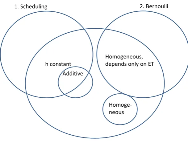
Figure 1. Relations between concepts in this paper
The findings of this paper are summarised in Figure 1. It looks perhaps a bit like a stylised Mickey Mouse, which is unintentional but amusing. The ears are the classes of scheduling and Bernoulli measures, respectively, while the head itself is the class of mean-dispersion models. The intersection between scheduling and Bernoulli is empty. The intersection between scheduling and mean-dispersion is the scheduling measures where ℎ is constant, such that any change in the mean travel time is fully reflected in the departure time. The measures in the intersection between Bernoulli and mean-dispersion are trivial, depending just on the mean travel time.
There are non-trivial homogeneous mean-dispersion measures and there are non-trivial additive scheduling or mean-dispersion measures, but any additive scheduling measure is also a mean-dispersion measure.
It might often be considered appropriate to require that a measure of the utility cost of travel time variability is consistent with underlying scheduling preferences, since these are defined over the travel outcomes that include the timing of a trip, and since such measures comprise an implicit choice of departure time. This rules out Bernoulli type measures as well as any homogeneous measure. Then, as noted, any measure with a constant reliability ratio is also ruled out.
On the other hand, there are situations where it is not appropriate to allow for an implicit choice of departure time. Such situations occur when information about current travel times is
v
1. Scheduling 2. Bernoulli
3. Mean-dispersion
Homogeneous, depends only on ET
Additive
v
14
revealed during a trip. In a dynamic route choice model where travellers gain information about travel times during the trip it seems more relevant to employ a scheduling model where the departure time is fixed. The model then becomes a Bernoulli type model. A useful constraint on that model may be derived from the assumption that the departure time was ex ante optimal with the information available before the trip was initiated. This kind of analysis seems not to exist in the literature and could be a subject for future research.
Scheduled transport services entail restrictions on the choice of departure times, since these are given by the schedule. In this case, the scheduling measures are not generally applicable, since these assume that the departure time can be chosen freely. In some cases, scheduling preferences still lead to simple cost measures even when the departure time is restricted by a schedule. Fosgerau and Engelson (Fosgerau and Engelson 2011; Engelson and Fosgerau 2011) show that a constant utility rate ℎ at the origin and an affine or constant plus exponential utility rate 𝑤 at the destination lead to a mean-dispersion measure in the case of a scheduled service plus a term that depends on the headway of the scheduled service.
In mode choice, one may assume that travellers choose departure time conditional on the choice of mode. In that case, measures based on scheduling preferences may be appropriate to account for the cost of travel time variability in the choice of mode.
Bernoulli type measures are based on a univariate cost function that depends only on the duration of a trip. This lack of structure may be considered an advantage. A possible view is that the scheduling model is overly restrictive. A restrictive assumption in that model is that scheduling preferences are pre-determined, they do not depend on the travel time distribution. However, scheduling preferences may actually be endogenous in the sense that they change as a consequence of a change in the distribution of travel times. Such models exist in the literature. Fosgerau and Small (2016) consider a situation in which scheduling preferences for the morning commute emerge endogenously in equilibrium, driven by the benefit each individual gains by synchronising his/her commute with other people. Fosgerau, Engelson and Franklin (2014) consider two people travelling to a joint meeting. Either traveller takes the travel time distribution of the other into account when forming his/her own scheduling preferences. Through equilibrium, the individual scheduling preferences then also depend on the travel time distribution faced by the individual. Another important, much overlooked but very intuitive insight of Fosgerau, Engelson and Franklin (2014) is that the cost of travel time variability derived using individual based measures such as those considered in this paper is only partial: it fails to take into account delays cost imposed on other people if the individual traveller does not fully internalise these costs in his/her preferences.
5. References
Abegaz, Dereje, Katrine Hjorth, and Jeppe Rich. 2015. “Testing the Slope Model of Scheduling Preferences on Stated Preference Data.” Working Paper.
Aczel, J. 1966. Lectures on Functional Equations and Their Applications. Academic Press. Bates, John, John Polak, Peter Jones, and Andrew Cook. 2001. “The Valuation of Reliability
for Personal Travel.” Transportation Research Part E 37 (2-3): 191–229.
15
Bernoulli, Daniel. 1954. “Exposition of a New Theory on the Measurement of Risk.”
Econometrica 22 (1): 23–36. doi:10.2307/1909829.
Börjesson, Maria, Jonas Eliasson, and Joel P. Franklin. 2012. “Valuations of Travel Time Variability in Scheduling versus Mean–-Variance Models.” Transportation Research Part B: Methodological 46 (7): 855–73. doi:10.1016/j.trb.2012.02.004.
Carrion, Carlos, and David Levinson. 2012. “Value of Travel Time Reliability: A Review of Current Evidence.” Transportation Research Part A: Policy and Practice 46 (4): 720– 41. doi:10.1016/j.tra.2012.01.003.
Cominetti, Roberto, and Alfredo Torrico. 2013. “Additive Consistency of Risk Measures and Its Application to Risk-Averse Routing in Networks.” arXiv:1312.4193 [math], December. http://arxiv.org/abs/1312.4193.
de Palma, A., and Nathalie Picard. 2005. “Route Choice Decision under Travel Time Uncertainty.” Transportation Research Part A: Policy and Practice 39 (4): 295–324. Engelson, Leonid. 2011. “Properties of Expected Travel Cost Function with Uncertain Travel
Time.” Transportation Research Record: Journal of the Transportation Research
Board 2254 (December): 151–59. doi:10.3141/2254-16.
Engelson, Leonid, and Mogens Fosgerau. 2011. “Additive Measures of Travel Time Variability.” Transportation Research Part B: Methodological 45 (10): 1560–71. doi:10.1016/j.trb.2011.07.002.
Feo-Valero, M., L. Garcia-Menendez, and R. Garrido-Hidalgo. 2011. “Valuing Freight Transport Time Using Transport Demand Modelling: A Bibliographical Review.”
Transp. Rev. 201: 1–27.
Fosgerau, Mogens. 2015. “The Valuation of Travel Time Variability.” International Transport Forum.
Fosgerau, Mogens, and Leonid Engelson. 2011. “The Value of Travel Time Variance.”
Transportation Research Part B: Methodological 45 (1): 1–8. doi:DOI:
10.1016/j.trb.2010.06.001.
Fosgerau, Mogens, Leonid Engelson, and Joel P. Franklin. 2014. “Commuting for Meetings.”
Journal of Urban Economics 81 (May): 104–13. doi:10.1016/j.jue.2014.03.002.
Fosgerau, Mogens, and A. Karlstrom. 2010. “The Value of Reliability.” Transportation Research Part B 44 (1): 38–49.
Fosgerau, Mogens, and Kenneth A. Small. 2016. “Endogenous Scheduling Preferences and Congestion.” International Economic Review Forthcoming.
Hjorth, Katrine, Maria Börjesson, Leonid Engelson, and Mogens Fosgerau. 2015. “Estimating Exponential Scheduling Preferences.” Transportation Research Part B: Methodological. Accessed September 14. doi:10.1016/j.trb.2015.03.014.
Johnson, M.B. 1966. “Travel Time and the Price of Leisure.” Western Economic Journal 4 (2): 135–45.
Li, Zheng, David A. Hensher, and John M. Rose. 2010. “Willingness to Pay for Travel Time Reliability in Passenger Transport: A Review and Some New Empirical Evidence.”
Transportation Research Part E: Logistics and Transportation Review 46 (3): 384–
403. doi:10.1016/j.tre.2009.12.005.
Lyman, Kate, and Robert Bertini. 2008. “Using Travel Time Reliability Measures to Improve Regional Transportation Planning and Operations.” Transportation Research Record:
Journal of the Transportation Research Board 2046 (September): 1–10.
doi:10.3141/2046-01.
Mas-Colell, A., M. Whinston, and J. Green. 1995. Microeconomic Theory. Oxford: Oxford Press.
Milgrom, Paul, and Ilya Segal. 2002. “Envelope Theorems for Arbitrary Choice Sets.”
16
Noland, Robert B., and Kenneth A. Small. 1995. “Travel-Time Uncertainty, Departure Time Choice, and the Cost of Morning Commutes.” Transportation Research Record 1493: 150–58.
Oort, O. 1969. “The Evaluation of Travelling Time.” Journal of Transport Economics and Policy 3: 279–86.
Small, K. 1982. “The Scheduling of Consumer Activities: Work Trips.” American Economic Review 72 (3): 467–79.
Small, Kenneth A. 2012. “Valuation of Travel Time.” Economics of Transportation 1 (1–2): 2–14. doi:10.1016/j.ecotra.2012.09.002.
Small, Kenneth A., Clifford Winston, and Jia Yan. 2005. “Uncovering the Distribution of Motorists’ Preferences for Travel Time and Reliability.” Econometrica 73 (4): 1367– 82.
Tseng, Yin Yen, and Erik T. Verhoef. 2008. “Value of Time by Time of Day: A Stated-Preference Study.” Transportation Research Part B: Methodological 42 (7-8): 607– 18. doi:DOI: 10.1016/j.trb.2007.12.001.
Vickrey, William S. 1973. “Pricing, Metering, and Efficiently Using Urban Transportation Facilities.” Highway Research Record 476: 36–48.