Munich Personal RePEc Archive
Economic Analysis of the Impact of
Development Aid : An Application of
Error Correction Modelling (ECM) to
Ethiopia
gebregergis, Cherkos Meaza
St. Mary’s University, TZG-general Development Research
Consultancy
30 September 2016
Online at
https://mpra.ub.uni-muenchen.de/83562/
Economic Analysis of the Impact of Development Aid : An
Application of Error Correction Modelling (ECM) to Ethiopia
Cherkos Meaza Gebregergis1 and Abis Getachew Mekuria2
Abstract
Foreign aid inflows have grown significantly in the post-war period. Many studies have tried to assess the effectiveness of aid at the micro- and macro-level. While micro evaluations have
found that in most cases aid „works‟, those at the macro-level are ambiguous. This paper investigates the impact of foreign aid on economic growth in Ethiopia using time series data for the period 1981 to 2015. The main objective is to identify the relationship that aid has with the developmental path of the country and whether one can reasonably link outcomes to aid inputs.
To this end, the study used the production function initiated by Solow-Swan model and cointegration analysis. The study is able to demonstrate the existence of long-run relationship between the official development assistance and economic growth of Ethiopia. The study found that there is negative relationship between ODA and economic growth in the short run and tend to be postive in the long run.
Key Words: Economic Growth, Official Developmen Assistance, cointegration analysis
1
St. Mary’s University and TZG-General Development Research Consultancy Company
[email protected] Mobile: +251967424446
2
Ethiopia Development and Research Institute(EDRI)
Introduction
Development aid, for this study, is referred to the official Development Aid (ODA3) where it is commonly defined according to Organization for Economic Cooperation and Development as
“financial flows, technical assistance, and commodities that are designed to promote economic development and welfare as their main objective and are provided as either grants or subsidized
loans”. The history of development aid goes back to the post-World War II era that aims to improve and bring economic growth to those underdeveloped nations. The Marshall-Plan4 targeting to reconstruct the war-torn economy of western Europe can be mentioned.
In recent years, aid to developing countries has increased massively and they receive billions of dollars per year in the form of aid from donors. The conclusion on aid effectiveness is doubtful among economists, found to be inconclusive, and has been a controversial subject for years. various time series and cross-country studies have come up with different results and different policy inferences. While some scholars point out the importance of good governance in order for recipient countries to benefit from aid, others highlight the lack of trust in aid, that is, whether
foreign aid has a positive correlation towards recipient country‟s economic growth. Foreign aid is a subject of an on-going debate that has led to diverse outcomes (Rajan et al, 2005).
A very important question nowadays is that does aid really work? if it does not really work, the justification is that there is no reason to provide aid, it would be withheld and at the extreme aid agencies should be closed down. The argument is also extended how far is official development aid effective and how is possible to see its impact at macro level (Riddell. 2014)
One argument that usually come into the mind of researchers who studied the effectiveness of aid is that there should be a mechanism to look at the after and before or with and without. In other words, the correct economic approach to capture aid-effectiveness is the difference between actual macroeconomic performance observed with aid program and the performance that would have been expected in the absence of such aid. To understand the impact of an action on an event, the basic question that requires being answered is that what would have happened to
3
Also can be defined as financial aid provided by governments and other agencies to support the economic,
environmental, social and political development of those developing countries.
4
Officially the European Recovery Program, ERP, American initiative to aid Western Europe rebuilding
war-devastated regions, remove trade barriers, modernize industries, make Europe prosperous again and prevent the
the event if an action did not take place given that all other circumstances are kept the same (Haque et al, 1998).
Ethiopia has been one of the major recipients of international aid since the imperial regime but there has been less economic growth and poverty remain inherent for many years in spite of the
notable donor interventions in the country‟s economy (Geda et al, 2011)
Generally speaking, poor countries lack the domestic resource to finance investment and capacity to import technology and capital goods, as a result aid is traditionally considered helpful to fill the gap that developing countries usually experience. The case for Ethiopia is not different from those cases. The ability of the country to improve the level of investment and promote economic growth with the domestic capital sources and private capital flows is not sufficient enough (Gomanee et al.2005)
Most of the research exploring the causality relationship between official development assistance and economic growth are done using cross-sectional method and wider in scope but this paper will attempt to see the impact of ODA on the economic growth of Ethiopia over extended periods of time because, it is believed that each country is unique, the role of aid can be understood best through careful analysis of individual countries. Finally, the study will be extended to include the current dominating debts on the effectiveness of aid mainly the “Big
Push” of Jeff Sachs5 or “Dead Aid” of Dambisa Moyo6
among others. To be more specific, the study will attempt to assess aid history of Ethiopia and its relationship with economic growth viz-a-viz “ dead Aid” of Dambisa Moyo.
5Jeff Sachs‟ new book “The End of Poverty” ( 2005) advocates a big
-Push” featuring large increase in aid to finance a package of complementary investments in order to end world poverty.
6Zambian born international economist and author where her first book was “Dead Aid: Why
Aid Is Not Working
2. Literature Reviews 2.1. Theoretical reviews
There are various factors which determine economic growth of a country. They include the quality of labour force, resources (natural and financial), capital, technology and the institutional setting of economic activities. Early economic growth theories in the 1950s and 1960s stressed that the basic
problem for many developing countries was precisely capital formation in achieving economic growth. Thus these theories were in the view that development assistance was important for these countries to fill the finance gap and technology gap. More popularly, these gaps were known as saving gap and the trade gap.
However, there are different views on the role of aid in filling the savings gap and the trade gap and thus contributing to growth in developing countries. In the following section, we are going to see the conclusions of H-D Model, Two-Gap and Three-Gap Models.
2.1.1. Harrod-Domar Model
The Harrod-Domar model, shows that output depends on the investment rate and the productivity of that investment. In an open economy, investment is financed by savings which is a sum of domestic and foreign savings. This model explains economic growth in terms of a savings ratio and
capital-output coefficient.
The incremental capital-output ratio (ICOR) gives how many units of additional capital are required to yield a unit of additional output, thus the ICOR is the ratio of investment ratio to the growth rate. The incremental capital-output ratio (ICOR) is thought to range between 2 and 5. A high ICOR is often taken as a measure of poor quality of investment.
minimize their dependence on aid, they need to increase their saving propensities which will increase funds required for investments.
2.1.2 The Two Gap Model
The standard model used to justify aid was the „two gap model‟ of Chenery and Strout (1966) which has been already referred to in the previous sections. In this model the first gap is between the amount of investment necessary to attain a certain rate of growth and the available domestic savings (the saving gap). The second gap is the trade gap or foreign exchange gap. Even though the saving investment gap would be small, a larger trade gap would undermine productive investment due to limited imports of capital goods needed for investment. It is argued that at any moment in time one gap is binding in aid recipient countries thus foreign aid is required to fill that gap. The assumption that aid fills these gaps will hold true only if investment is constrained by liquidity but the incentives to invest are favorable. If the cause of low investment is the poor incentives to invest, then aid will not increase investments as it will finance consumption rather than investment. Furthermore, the effectiveness of aid in filling these gaps will depend on the productivity of the investments made.
2.1.3. Three Gap Model
The three gap model, refers to the saving- investment gap, trade gap and the fiscal gap. The fiscal gap refers to a gap between government revenues and expenditures although the fiscal gap is a subset of the saving gap. Due to this fiscal gap, government efforts to stimulate private investment may be restrained when government resources for investment and imports are insufficient, among other things, as a result of debt service. The closing of this fiscal gap may be facilitated by external resources directed to the government budget.
In contrast, if aid is in form of a loan and not a grant, may have adverse implications for the savings, foreign exchange and fiscal gaps in the long-run and for the macroeconomic performance in general. A loan aid inflow may fill the trade gap today, but necessitates a faster rate of export growth in the future for the country to become independent of foreign. Also debt
government investment, particularly in infrastructure, education and health facilities, a factor which is likely to affect negatively private investments.
2.2. What Do Previous Studies Tell us about Aid and Growth?
In this section a survey of previous studies is made to establish the inconclusive nature of the existing empirical evidences both in a country wise and across group of countries and to justify the need for another empirical study on the same subject area. A lot of empirical works have been made to examine the relationship between development aid and economic growth of recipient country complemented by case study evidence at project levels. But the result of those various studies are found to be mixed where some researchers conclude there exist positive relationship, while others found a negative association and others still concluded neither negative nor positive correlation between the two variables.
The aid-growth literature is subjugated by cross-country studies of growth regression and has also been criticized for methodological problems. Those cross sectional studies on the relationship between aid and growth of the area ends with inconclusive results. That is most of these cross sectional analysis suggest that the growth impacts of foreign assistance vary among countries that pointed out the need for empirical study for individual countries. Therefore, the main idea here is to inspect the possible relationship between development aid and economic growth in time series of country-specific growth regression. Unlike the cross-country growth regressions which puts a number of heterogeneous countries with different economic policy environment, institutional setup, natural resource endowment, and others altogether, this study analyses the impact of foreign aid on economic growth in the context of Ethiopia.
Gomanee et al (2005) attempted to investigate the impact of aid on economic growth 25 selected sub-Saharan African countries by using residual regressors approach on the pooled data collected for the period 1970 to 1997. They have identified three mechanisms of transmission where aid can be channeled to economic growth: investment7, import financing and government spending. The researchers found a significant and positive effect of foreign aid on economic growth. Each one percentage increase in the aid/GNP ratio contributes one quarter of one percentage point to growth rate on average holding other things constant. Finally, they concluded that African poor economic growth performance should not be related to aid ineffectiveness. Bhattarai (2005) uses time-series data of Nepal for the period 1970-2002, and employs cointegration and the error correction mechanism as the estimation procedure to examine the effectiveness of aid and its link with domestic saving, investment and per capita growth. The results show that aid has a positive and significant relationship between per capita real GDP, savings and investment in the long-run. He also found that aid effectiveness improves economic growth in times of good policy environment, that is, an economy which is characterized by a stable macro-economy, openness to trade and a liberalized financial sector. Moreover, the study also found that bilateral and multilateral aid are equally effective in the long-run. However, grants has a stronger positive association with per capita real GDP in the long-run than loans.
Birara (2011) has examined the impact of foreign aid on economic growth and the transmission mechanisms of Ethiopia using Johansson Maximum Likelihood approach for the period 1970/71 to 2008/09. The co integration test result indicates the existence of long run relationship among the variables8 entered in his models. In the long run foreign aid has a positive and significant impact on growth through its significant contribution to investment and import. However, the dynamic short run model points out that in order aid to have significant impact on growth it has to be assisted by good monetary, fiscal and trade policy.
Wondwesen(2003) analyzed the impact of foreign aid on growth on annual data covering the
period 1962/63 to 2000/01 applying Johansen‟s maximum likelihood technique found that aid
has significant contribution to investment both in the short run and long run. Aid is found to be
7
Gomanee et al (2005) identify investment as the most significant transmission mechanism among others.
8
The explanatory variables includes Level of investment that is not financed by aid, foreign aid, policy index times
ineffective in enhancing growth. However, he found that when aid is interacted with policy, the growth impact of aid found to be significant that is, aid is conditional on quality policy environment. His result further implied that attention should be focused on improving the existing macroeconomic policy environment for an inflow of aid to be used effectively.
Tadesse T (2011) has examined the impact of foreign aid on investment and economic growth in Ethiopia over the period 1970 to 2009. The researcher employed multivariate cointegration analysis while conducting his study. Foreign aid is effective in enhancing growth. The empirical result from the investment equation displays that foreign aid has a significant positive impact on investment in the long run. On the other hand, volatility of aid has a negative influence on domestic capital formation activity by creating uncertainty in the flow of aid. On the other hand, the aid-policy interaction term has produced a significant negative effect on growth which means bad policies negatively affects the aid effectiveness. The growth equation also revealed that rainfall variability has a significant negative impact on economic growth.
Rajan (2005) examined the effects of aid on growth using cross-sectional and panel data for selected poorer countries. The data are observed and labeled as follows. Countries are included in the sample for the 1960-00 horizon if there are data for at least 35 years; for the 1970-00 horizon for at least 25 years of data; for the 1980-00 horizon for at least 15 years of data; for the 1990-00 horizon for at least 5 years. The researcher found little robust evidence of a positive (or negative) relationship between aid inflows into a country and its economic growth. He also found no evidence that aid works well in better policy or geographical environments, or that certain forms of aid work better than others. His main findings, which relate to the past, do not imply that aid cannot be beneficial in the future. But he suggested that for aid to be effective in the future, the aid apparatus will have to be rethought.
studies to investigate the possible channels through which foreign aid can have positive influence on growth.
Burnside et al (1997) used a new database on foreign aid to examined the relationships among foreign aid, economic policies, and growth of per capita GDP. In panel growth regressions for 56 developing countries and six four-year periods (1970-93) the policies that have a large effect on growth are fiscal surplus, inflation, and trade openness. They constructed an index of these three policies, interact it with foreign aid, and instrument for both aid and aid interacted with policies. They found that aid has a positive impact on growth in developing countries with good fiscal, monetary, and trade policies. In the presence of poor policies, on the other hand, aid has no positive effect on growth. This result is robust in a variety of specifications that include or exclude middle-income countries, include or exclude outliers, and treat policies as exogenous or endogenous. They examined the determinants of policy and find no evidence that aid has systematically affected policies - either for good or for ill. They also estimated an aid allocation equation and show that any tendency for aid to reward good policies has been overwhelmed by
donors‟ pursuit of their own strategic interests. In a counterfactual they reallocated aid, reducing
the role of donor interests and increasing the importance of policy: such a reallocation would
have a large, positive effect on developing countries‟ growth rates. 2.3. Ethiopia Overall Ecomnomic Performance
Fig 2.1: GDP growth of Ethiopia taken from NBE data base
As it is shown in the above figure, the economy of the country is growing with time with the exception of the early 2000s. In the early periods, the economy growth declines and reaches a negative figure in 2003. These decline in the growth are mostly associated with Ethio-Eritrea war which caused a lot of damages in human life as well as in materials. However, the economy started to grow in an increasing rate which is about 11.7% in 2004 and showed a positive growth for the consecutive 10 years ranging from 8.7 % in 2012 and 13.5% in 2011. This consistent and promising growth has enabled the country to maintain an average annual economic growth rate of 11 percent over the last 12 consecutive years between 2003/04 and 2014/15.
However, the high import intensity of the economy, limited capacity to produce capital goods, low levels of domestic savings and limited capacity to generate foreign exchange are considered to be the bottlenecks to the development effort of Ethiopia. All these factors have provided an apparently objective justification for the huge inflow of foreign aid. Consequently, foreign aid has been playing a critical role in the development efforts of Ethiopia since the 1950s. Like the case for all poor countries, development aid has been flowing to Ethiopia since the mid-20th century. Those development aid are considered as the means to finance deficits, filling the trade gap, saving gap by expanding the level of investment of the country.
increasing efforts were made to mobilize foreign aid in the last two regimes. Following the change in political regime in 1991 and the adoption of the structural adjustment program in 1992/93 in particular, the country has enjoyed a significant amount of aid (Alemu 2009).
Nowadays, Ethiopia has been one of the major recipient of international aid. According to the OECD-DAC Statistics, Ethiopia has received a net official development assistance of US $2.03 billion in 2006 making the country the 4th largest recipient from the African countries next to Nigeria, DR Congo and Sudan. In absolute term, ODA to the country has averaged around US$3.3 billion over the last nine years (2006 – 2014). Figure 2.2 shows the trend of development aid to Ethiopia for the recent 35 years. The trend is increasing slowly in the 1980s and early 1990s and started to decline during the period of war with Eritrea. As discussed in the above, the country has enjoyed a very increasing foreign assistance after the adoption of Structural Adjustment Programs of the world dominant financial organizations, IMF and WB.
3. Methodological Issues 3.1. Model Specification
To investigate the impact of development assistance on economic growth of Ethiopia, this study applies a time series approach for the period 1991 to 2014 and the Swan Solow model has been employed to estimate the growth effect of foreign aid. The neo classical Solow model articulated economic growth is resulted from the combination of capital and labor. The total factor productivity which is referred to as Solow residual also encompasses all other factors that accounts output growth. Thus, the general equilibrium model for this study can be presented in the Cobb-Douglas production form with constant return to scale with respect to capital and labor as follows.
Yt = F(At, Lt, Kt) ………..(3.1)
Where: , represents total output, physical capital, labor force and technological progress or total factor productivity9 (TFP) at time t respectively. A production function which follows the specification in (3.1) can be decomposed to determine the contribution of each
9
The Total Factor Productivity variable consists of all other variables other than those included in the model and
variable to economic growth. Suppose an economy can be described by a Hicks neutral Cobb-Douglas production function of the form,
Yt = AtLtβ1K tβ2………..(3.2)
Where: 0 < β1 < 1 and 0 < β2 < 110
The study extends the Cobb-Douglas production function11 in to a detailed version by assuming that Total factor Productivity is determined by level of development assistances, international trade and skilled human power. I assume that the increase of development assistance inflows increase the total factor productivity which in turn raises the rate of overall economic growth of Ethiopia. Morrisey(2001) has pointed that foreign aid can contribute to economic growth through increase in physical and human capital investment, increases the capacity to import capital goods or technology and is associated with technology transfer. International trade is believed to contribute positive impact on economic growth by efficient allocation of internal and external resources, shift of technological advancements from developed countries to developing economies and less developed countries practice the innovations by developed countries i.e.
learning by doing effects12. Similarly, the presence of skilled human power in a country means
there will be higher potential to originate and innovate new goods and services which can stimulate the economy. Expressing the technological progress as a function of trade openness, development aid, skilled human power and other external factors given as;
At = F(ODAt, TOt, Ht) ……….(3.3)
Where: ODAt, TOt and Ht are official development aid, trade openness measured as the ratio of
trade (import and export) to GDP and skilled human power at time t respectively.
The above expression can be arranged as follows‟
At= β0ODAtβ3TOtβ4Htβ5……….(3.4)
10
Note that the coefficients and represents the marginal effects labor and capital on output respectively. 11
The standard growth model can be also rewritten as follows after logarithmic transformation
12
Learning by doing implies that greater investments in certain sectors increases the experience of firms, workers,
Where: β0 is time invariant constant
0 < β3 < 1, 0 < β4 < 1 and 0 < β5 < 1
Upon substitution of the expression 3.4 for TFP in to the Solow growth model of 3.2, we will have the following general appearance.
Yt = β0 Ltβ1 K tβ2 ODAtβ3TOtβ4 Htβ5………..(3.5)
The study specifies the model to be estimated by transforming in to natural logarithmic form, therefore the above equation can be explained as;
lnGDPt= β0 + β1lnLt + β2lnK t +β3lnODAt +β4lnTOt +β5lnHt+ εt………..(3.6)
There are five deterministic sources of economic growth in equation (3.6) : labor, physical capital, official development aid, trade openness and human. Of interest in this paper is the sign of the parameter 𝛽3 which is the marginal effect of ODA to economic growth. Since all variables
are expressed in terms of natural logarithms then the coefficients can be interpreted as elasticities and the variables are expressed in growth terms.
If the six variables including the proxy for economic growth in equation (3.6) are cointegrated then one can find an expression that defines the long run relationship between natural logarithm of GDP and the other five variables, although this has to be tested formally. Thus, the model can be generally expressed in terms of a long-run or cointegrating relationship given by:
𝐹(𝑌𝑡,K𝑡,Ht,𝑂𝐷𝐴𝑡,L𝑡 ,TO𝑡) = 0 ...(3.7)
Where 𝑌𝑡 is the natural logarithm of GDP or growth rate of GDP, K𝑡 and Ht are the natural
logarithm of physical and human capital respectively, 𝑂𝐷𝐴𝑡 is the natural logarithm of official development assistance, L𝑡is the natural logarithm of labor force and TOt is the natural logarithm
of trade openness.
3.2. Co-Integration
An essential exception arises when the two nonstationary series have the same stochastic trend in common. Consider two series, integrated of order one, Yt and Xt , and suppose that a linear
relationship exists between them. This is reflected in the proposition that there exists some value
β such that Yt−βXt is I (0), although Yt and Xt are both I (1). In such a case it is said that Yt and
Xt are cointegrated, and that they share a common trend. Although the relevant asymptotic theory is nonstandard, it can be shown that one can consistently estimate β from an OLS regression of Yt on Xt.
An important issue in econometrics is the need to integrate short run dynamics with long run equilibrium. The desire to evaluate models which combine both short-run and long-run properties and which at the same time maintain stationarity (i.e., which are non-trended), has prompted a reconsideration of the problem of regression using variables measured in their levels.
This „reconsideration‟ the product of breakthroughs in econometric theory in the past 15-20 years or so has given rise to cointegration methods and error correction models.
If the economic series have become non-stationary at level and have the same integration order then co-integration becomes an overriding requirement for any economic model. Mostly, a null hypothesis of there is no cointegration or long run relationship between variables in the model against the alternative hypothesis of the null hypothesis is not true will be tested using the Johansen cointegration test. Besides, Engle Granger test is strong in the case of bivariate analysis. It is then possible to test for cointegration among the variables using the ADF unit root test on the residuals(
ε
t) estimated from the cointegrating regression between Yt and Xt (equation3.10). Let us consider that we have the following equation.
Yt= β0+ β1Xt +
ε
t ...(3.8)To examine whether
ε
t is I(0) or I(1), we should obtain the values of the error term from theWhen the variables or series are having cointegrated relationships then the linear combination of these series would be stationary and gives long relationship between the variables. The ECM is a convenient model measuring the correction from disequilibrium of the previous period which has very good economic implications.
The Granger representation theorem (Granger, 1983; Engle and Granger, 1987) states that if a set of variables are cointegrated, then there exists a valid error-correction representation of the data. Thus, if Yt and Xt are both I (1) and have a cointegrating vector (1,−β)‟, there exists an error-correction representation, with εt = Yt −βXt, of the form:
ΔYt = δ +
φ1ΔXt
−1−γ
(Yt−1−βXt−1) +ε
t ...(3.9)where the error term has no moving average part and the systematic dynamics are kept as simple as possible. Intuitively, it is clear why the Granger representation theorem should hold. If Yt and
Xt are both I (1) but have a long-run relationship, there must be some force which pulls the
equilibrium error back towards zero. The error-correction model does exactly this: it describes how Yt and Xt behave in the short-run consistent with a long-run cointegrating relationship. If
the cointegrating parameter β is known, all terms in the above expression are I (0) and no
inferential problems arise.
4. Results and Discussion 4.1. Stationarity Test
Prior to testing for cointegration and estimating the long run equation explaining growth and ODA in Ethiopia, it is necessary to examine whether the data series is stationary in level, or stationary in differences using ADF test in order to apply the correct methodology. Testing for stationarity also helps to avoid any spurious inferences.
In case of testing variables in their level, the ADF test is performed with constant as well as with constant and trend whereas the ADF test of unit root is done without constant and with constant for the differenced variables. The detail of the test is summarized in the table below.
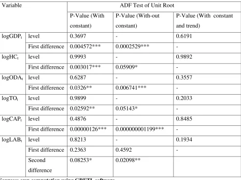
Table 4.1: Augmented Dickey Fuller Test of variables for unit root
Variable ADF Test of Unit Root P-Value (With
constant)
P-Value (With-out constant)
P-Value (With constant and trend)
logGDPt level 0.3697 - 0.6191
First difference 0.004572*** 0.0002529*** - logHCt level 0.9993 - 0.9892
First difference 0.003017*** 0.05909* - logODAt level 0.6287 - 0.3557
First difference 0.0326** 0.006741*** - logTOt level 0.9899 - 0.2033
First difference 0.02592** 0.05143* - logCAPt level 0.4876 - 0.8485
First difference 0.00000126*** 0.000000001199*** - logLABt level 0.8213 - 0.1934
First difference 0.2363 0.4592 - Second
difference
0.08253* 0.02098**
Sources: own computation using GRETL software
Note: H0: Unit root, H1; No unit root, alpha level (α=0.05)
***, ** and * indicates the rejection of the null hypothesis of unit root at 1%, 5% and 10% respectively.
Co-Integration Analysis
Johansen’s Cointegration Test Result
From the stationarity test discussed in the previous section, it is found that all variables except labor variable are stationary at their first differenced and are the same order, I (1). Besides, we have found that there is an evidence showing the long run association between the variables according to the Engle-Granger test of cointegration. But this type of test is mostly criticized in case there are more than two variables, that is the problem of uniqueness. Thus, to avoid this problem a Johansen test is required to determine how many cointegrating vectors there are for a set of variables.
The cointegration test proposed by Johansen (1988) and Johansen and Juselius (1990) requires that the optimal lag length must be determined before testing. The optimal lag length is determined from the unrestricted vector auto-regression equation that minimizes the Akaike Information Criterion (AIC) or Schwarz Information Criterion (SIC) or Hannan-Quinn Criterion (HQC). In doing so, the maximum lag order is set to be 4 recommended by the software and later decided to be 1, the lag which is minimum. (See annexed table)
Long-Run Estimates
Since the variables are cointegrated then one can determine the long run estimates for the relationship
between official development assistance and economic growth. Table 4.6 presents the normalized cointegrating coefficients guided by the results of the cointegration tests.
long run normalized (β) Coefficients
Variables logGDPt logCAPt logHCt logODAt logTOt Coefficient (β) 1.0000 -0.4976 0.75057 0.35279 -0.23774 St.Error 0.0000 (0.26561) (0.32525) (0.15604) (0.18237)
Source: own calculation using GRETL software package
and skills of people. The government of Ethiopia has been investing on people‟s education and
this inturn initiates the economic growth to grow forward and positively.
This study found that trade openness, a proxy for the degree of trade liberalization comes to affect the economic growth negatively. This is probably due to the infant industry argument where government is uspposed to protect from external competition. Most of manufacturing industries are small and medium enterprises that their financial and production capacity is limited. Therefore, in times of liberalization those enterprises will face strong competition from external companies, they will immediately liquidate or demolished. Another reason may be the existence of bureaucratic, rent seeking behavior and corrupted individuals, public and private institutions wich they fail to facilitate every processes for the benefits of the country.
Official development assistance is affecting RGDP positively as of the study by Bhattarai (2005) who studied the relationship of those two variables for Nepal case and Birara (2011) a study for the case of Ethiopia. This paper basically shows how much aid is effective in terms of bringing postive economic growth in Ethiopia. Helping others who are in a need of it means putting
“plaster in a wound” which atleast can minimize the pain. Similarly foreign aid may not a sustainable solution but still it is contributing a lot in the developing countries by saving millions of life, as of the case for Ethiopia, it is also making the economy to step forward. It is very common to observe that many individuals travel for longer hour on foot, horse or other traditional transportation system to get social services including education and hospitals due to shortage of those infrastructures in nearest possible area.
Error Correction Model and Short Run Elasticities
Since the explanatory variables are found to be cointegrated, one can proceed to find the Error Correction Model (ECM) which also represents the short run relationship among the variables under study. Table 4.7 summarizes the error correction model as well as the short run elasticities of the variables, that is the short run effects of the explanatory variables on the economic growth of the country. The ECM is economically and statistically meaningful in the sense that it is negative and less than one. Therefore, according to the regression, the error correction term
Error Correction Model and Short Run Elasticities
--- coefficient std. error t-ratio p-value
--- const −0.195217 0.0643068 −3.036 0.0054 ***
d_l_GDPt-1 0.535350 0.238833 2.242 0.0337 **
d_l_CAP t-1 −0.218525 0.136951 −1.596 0.1227
d_l_HC t-1 0.147587 0.171814 0.8590 0.0982 *
d_l_ODA t-1 −0.00337086 0.0782985 −0.04305 0.0460 **
d_l_TO t-1 0.191342 0.140450 1.362 0.1848
EC t-1 −0.269958 0.106651 −2.531 0.0178 **
---
Mean dependent var −0.013623 S.D. dependent var 0.122043
Sum squared resid 0.214492 S.E. of regression 0.090828 R-squared 0.549976 Adjusted R-squared 0.446124 rho 0.013313 Durbin-Watson 1.841384
In addition to the adjustment speed, this short dynamics shows the individual effects of the
explanatory variables. For instance; last year‟s RGDP is showing positive and significant impact on current year RGDP that is, for every one percent change in the last year‟s RGDP, the current
RGDP changes in about 0.54 percent on average, Ceteris Paribus. In contrast, last year ODA comes to affect the current year RGDP inversely and it is also statistically significant. This can be due to the fact that the effect of aid comes to be effective with longer time span. In the short
run, last year‟s gross fixed capital formation and trade openness comes to affect the RGDP negatively and positively respectively but both are found to be statistically insignificant.
45 percent (using Adjusted R2) of variations in the dependent variable is explained by the variations in the explanatory variables included in the model. The Durbin-Watson statistic is also showing that we fail to reject the null hypothesis of error terms are not serially correlated.
5. Conclusion and Recommendation 5.1. Conclusion
Developing countries have a deficiency of domestic resource to finance investment and capacity to import technology and capital goods that is why it is mostly common to see those countries recieving billions of dollar in the form of grants and loans from the developed world. The case for Ethiopia is not different from those circumstances as the flow of ODA coming to country dramatically increased for the last two decades. Eventhough there has been a bulky of literature on the subject with different methodologies, the area remains to be debatable among the researchers.
The study has examined the economic analysis of the impact of development aid in Ethiopia. More specifically, the study has attempted to investigate whether there is long run relationship between official development aid and economic growth of Ethiopia for the time period extended from 1981 to 2015. To do so, multivariate cointegration technique is employed for the analysis of the long run relation where VECM analysis is used to assess the short run relationships and its linkage with the long run equilibrium path.
As it has been discussed many times so far, the prerequisite for cointegration analysis is that the variables need be stationary and integrated of the same order, the series is tested for unit root and the result found indicated that all the variables in the specified model except the explanatory variable labor are stationary after first difference i.e. I(1). eventually, cointegration test using Engle-Granger two step estimation for bivariate case and Johansen cointegration test has performed and the result satisfied the presence of long run relationship among the variables in the model.
on the economic growth of the country. Besides, the paper showed that the variables physical capital and trade openness exist to affect economic growth negatively.
Generally, since we are living in the world where assisting others who are in a need of the help is a culture. This study is also in favor of foreign aid.Who knows best about a patient: the doctor or the patient? Therefore, whatever the degree of aid effectiveness is, it is found that aid is helping developing countries in general and Ethiopia in specific by saving lives of millions of people, bringing positive economic growth and other related contributions.
5.2. Recommendation
Based on the empirical conclusions, the study is able to forward the following reasonable recommendations to be taken by the government of Ethiopia.
Including Ethiopia, the economy of developing countries is basically characterized by low level of saving, very huge trade and budget deficits. For this reason, the government need to use development aid as a main mechanism to finance those gaps that their country is experiencing persistently and eventually bring positive economic growth. But the development aid is required to be invested in the most productive sectors (investment areas) including agriculture, infrastructural developments and other areas which inturn stimulates the economy as a whole. In addition to this, the government need to minimize the bureaucratic nature and rent seeking behavior of individuals and institutions which limits the effectiveness of aid.
Where as the donors should also have a clear cut follow up commitment that tracks the progress of every dollar granted to the developing countries in general. Otherwise all those billions of dollars coming from the developed world may attract extra interest from the governing body to be corrupted. It should not be granted in a reciprocity principle where donors give aid to countries in an exchange or expectation of something to get back from them. The conditionality for granting aid is sometimes challenging to met and as a result those should be minimized as far as possible.
Finally, further investigations on the effectiveness of ODA at sector specific, in regional level, inclusion of new variables in to the model, the use of non-linear model specification and methodology is highly recommended. Besides, the inconsistencies of data reported by national institutions (including NBE and MoFED) as well as figures reported by WB, IMF, OECD and others needs to be harmonized as much as possible.
References
Alemu G. (2009), “A Case Study On Aid Effectiveness In Ethiopia; Analysis Of The
Health Sector Aid Architecture”, Wolfensohn Center For Development Working Paper 9
Arndt C., Jones S. and Tarp F. (2006), “Aid and Development: The Mozambican Case”,
Studiestræde 6, DK-1455 Copenhagen K., Denmark
Bhattarai B. (2005), “The Effectiveness of Foreign Aid: A Case Study of Nepal”,
University of Western Sydney, Sydney, Australia.
Birara Y. (2011), “The Impact Of Foreign Aid On Economic Growth In Ethiopia”,
Master thesis, AAU.
Bitew T. (2014), “Foreign Aid and Economic Growth in Ethiopia”, Unpublished Thesis, AAU
Boone, P. (1994), “The Impact of Foreign Aid on Savings and Growth”, London Schoolof Economics
Burnside, C. and Dollar, D. (1997), “Aid, Policies and Growth”, Policy Research
Working Paper 1777, World Bank, Washington, D.C
Burnside, C. and Dollar, D. (2000), “Aid, Policies and Growth”, American Economic
Durbarry R., Gemmell N. and Greenaway D (1998), “New Evidence on the Impact of
Foreign Aid on Economic Growth”, Centre for Research in Economic Development and International Trade, University of Nottingham
Easterly W. (2003), “Can Foreign Aid Buy Growth?”, Journal of Economic
Geda, A. and Tafere, K. (2011), “Official Development Assistance (Aid) and its Effectiveness in Ethiopia”, IAES working paper A07/2011
Gomanee K., Girma S. and Morrissey O. (2005), “Aid and Growth in Sub Saharan
Africa: Accounting for Transmission Mechanisms”, Research paper No. 2005/60, United
Nation University.
Haque, N. and Khan, M. (1998), “Do IMF-Supported Programs Work: A Survey of Cross- Country Empirical Evidence”, IMF Working Paper/98/169/
Holden K. and Thompson J. (1992), “Co-Integration; An Introductory Survey”, British Review of Economic Issues, volume 14, No 33
http://www.nber.org/papers/w11513
IMF (2015), IMF, Ethiopia‟s Country Report No. 15/326
Kim J. (2006), “The Impact of Foreign Aid on Economic Growth in Developing countries”, Sogang University
Liew Y., Mohamed R. and Mzee S. (2012), “ The Impact of Foreign Aid on Economic
Growth of East African Countries”, Journal of Economics and Sustainable Development,
Vol.3, No.12
Mosley P., Hudson J, and Sara H. (1987), “Aid, the Public Sector and the Market in Less Developed Countries”, The Economic Journal, Vol. 97, No. 387
Online at https://mpra.ub.uni-muenchen.de/33953/
Papanek G. (1973), “Aid, Foreign Private Investment, savings, and Growth in Less Developed Countries”, Journal of Political Economy 81(1): 120-130.
Rajan G. and Subramanian A. (2005), “Aid And Growth: What Does The Cross-Country
Evidence Really Show?”, NBER Working Paper No 11513, Massachusetts Avenue, Cambridge Review, Vol. 90, pp. 847-68
Riddell, R. (2014), “Does Foreign Really Work?”, Oxford Policy Management, oxford, UK
Tadesse T. (2011), “Foreign aid and economic growth in Ethiopia” MPRA Paper No.
33953.
White H. and Luttik J. (1994), “The Countrywide Effect of Aid‟‟, WB policy Research
Working Paper No 1337
Wondwossen T. (2003), “An empirical investigation of the Aid-growth relationship in
Johansen test for cointegration
Rank Hypothesis Eigen value Trace test P-value Lmax test P-value Null Alternative
0 H0 = 0 H1 =1 0.65932 69.939 [0.0470]** 36.611 [0.0192]**
1 H0 <= 1 H1 =2 0.33550 33.327 [0.5432] 13.897 [0.8243]
2 H0 <= 2 H1 =3 0.30837 19.431 [0.4732] 12.536 [0.5095]
3 H0 <= 3 H1 =4 0.18342 6.8951 [0.5958] 6.8894 [0.5107]
4 H0 <= 4 H1 =5 0.00016685 0.0056734 [0.9400] 0.0056734 [0.9400]
Lag length Selection criteria using AIC, SIC and HQC
lags AIC SIC HQC loglik P(LR) 1 -6.464472 -5.076742* -6.012107 130.19931