University of Warwick institutional repository: http://go.warwick.ac.uk/wrap
This paper is made available online in accordance with publisher policies. Please scroll down to view the document itself. Please refer to the repository record for this item and our policy information available from the repository home page for further information.
To see the final version of this paper please visit the publisher’s website. Access to the published version may require a subscription.
Author(s): David L. Cheung
Article Title: Molecular dynamics study of nanoparticle stability at liquid interfaces: Effect of nanoparticle-solvent interaction and capillary waves
Year of publication: 2011 Link to published article:
http://dx.doi.org/10.1063/1.3618553
Publisher statement: Copyright © 2011 American Institute of Physics. Citattion: Cheung, D.L. (2011). Molecular dynamics study of
Molecular dynamics study of nanoparticle stability at liquid
interfaces: effect of nanoparticle-solvent interaction and capillary
waves
David L. Cheung∗
Department of Chemistry and Centre for Scientific Computing,
University of Warwick, Coventry, CV4 7AL, UK
Abstract
While the interaction of colloidal particles (sizes in excess of 100 nm) with liquid interfaces may
be understood in terms of continuum models, which are grounded in macroscopic properties such as
surface and line tensions, the behaviour of nanoparticles at liquid interfaces may be more complex.
Recent simulations [D. L. Cheung and S. A. F. Bon, Phys. Rev. Lett., 102, 066103 (2009)] of nanoparticles at an idealised liquid-liquid interface showed that the nanoparticle-interface
interac-tion range was larger than expected due, in part, to the acinterac-tion of thermal capillary waves. In this
paper molecular dynamics simulations of a Lennard-Jones nanoparticle in a binary Lennard-Jones
mixture are used to confirm that these previous results hold for more realistic models.
Further-more by including attractive interactions between the nanoparticle and the solvent it is found that
the detachment energy decreases as the nanoparticle-solvent attraction increases. Comparison
be-tween the simulation results and recent theoretical predictions [H. Lehle and M. Oettel, J. Phys.
Condens. Matt., 20, 404224 (2008)] shows that for small particles the incorporation of capillary waves into the predicted effective nanoparticle-interface interaction improves agreement between
simulation and theory.
I. INTRODUCTION
The adsorption of nanometre-sized particles, including nanoparticles, polymers or den-drimers and proteins, at soft interfaces has attracted much scientific interest1 and is central to a number of emerging technologies. Adhesion at air-water and oil-water interfaces po-tentially provides an elegant method for the preparation of dense, ordered nanoparticle structures2, and the modification of interfacial properties by the adsorption of nanoparti-cles may be used to stabilise micron-scale structures such as nanoparticle-armoured fluid droplets3 or phase-arrested gels4. As well as synthetic nanoparticles the behaviour of biolog-ical objects such as proteins5 or virus capsids6 at liquid interfaces have also been the subject of investigation.
Due to the experimental interest in these systems the behaviour of nanoparticles at liquid interfaces has been studied theoretically, both using analytic and semi-analytic theories and molecular simulations. The adhesion of solid particles to liquid interfaces has long been understood as a result of particle wettability and changes in interfacial area7,8. The theory of colloidal adhesion on liquid interfaces has been thoroughly developed, including both the effect of particle fluid surface tensions9,10 and line tension11. These models are typically derived from considering colloidal (200-1000 nm) sized particles and so are grounded in macroscopic quantities such as surface and line tensions, and neglect microscopic phenomena such as capillary waves. One common model is the Pieranski approximation8 in which the free energy is given simply in terms of changes to the interfacial area (AAB) and the area of
the nanoparticle in contact with the two fluid components (AiN) as
F(zc) =−γABAAB+γANAAN+γBNABN
=πγABzc2+ 2πR
2
c(γAN−γBN)(1−zc/Rc) (1)
where zc is the distance between the interface and the colloid center, γAB is the A-B
in-terfacial tension, γiN is the surface tension between the nanoparticle and fluid i, and Rc is
the nanoparticle radius. This was then extended by Aveyard and Clint (AC) to include line tension11, giving
F(zc) =πγABzc2+ 2πR
2
c(γAN −γBN)(1−zc/Rc) + 2πτ Rc
p
1−(zc/Rc)2. (2)
on the nanoparticle-interface interaction12and interface mediated nanoparticle-nanoparticle interactions13,14.
The adsorption of nanoparticles on liquid interfaces has also been studied using molec-ular simulations. In pioneering work Bresme and Quirke employed molecmolec-ular dynamics simulations to study the effect of line tension on the stability of nanoparticles at liquid interfaces15–17. More recently the interaction potential between a nanoparticle and a liq-uid interface was determined using Monte Carlo or molecular dynamics simulations, for uniform18, Janus (amphiphilic)19, and polymer-grafted nanoparticles20. Simulations have also been used to study the interactions between adsorbed nanoparticles21, self-assembly of nanoparticles at liquid-liquid interfaces22, and nanoparticle diffusion at interfaces23,24. Density functional theory has also been recently used to study the interaction and wetting behaviour of nanoparticles at fluid interfaces25,26.
significantly smaller than that of a typical liquid mixture. It is then natural to ask how applicable these findings are to other, more realistic, fluid models.
In this paper, the interaction between a nanoparticle and a liquid interface, modelled in this case by Lennard-Jones interactions, is studied using molecular dynamics simulations. While the Wang-Landau MC simulations31 that were used in previous work18,19 may be applied in this case, they may be inefficient when applied to complex molecular systems, and in the case of very large free energy barriers the time required to determine a converged weight function may be prohibitively long. Molecular dynamics simulations are more easily generalised to complex systems, and may be easily parallelised to take advantage of modern parallel computers. Free energy profiles may be determined using methods such as umbrella sampling32, steered molecular dynamics33, metadynamics34 or adaptive biasing force35, the latter two being conceptually similar to the Wang-Landau MC methodology used previously. In this paper molecular dynamics simulations are used to study the stability of a spherical nanoparticle at a model liquid-liquid interface. The free energy profile was determined using umbrella sampling, a simple and robust method for this purpose. As well as testing the validity of the results of Ref18 for more realistic fluids, the effect of attractive nanoparticle-solvent interactions and the effect of capillary waves on the interaction will be examined. Details of the computational model and methodology are given in the following section, the results of the simulations are presented and discussed in Sec. III, while Sec. IV gives some conclusions and avenues for further work.
II. MODEL AND METHODOLOGY
The solvent is modelled as a two-component fluid, interacting through a cut and shifted Lennard-Jones potential
VS(r) =
4ǫh σ
r
12
− σ r
6i
−Vcut, r≤rcut
0, r > rcut
(3)
where Vcut = 4ǫ[(σ/rcut)12 −(σ/rcut)6] and rcut = 2.5σ for like particles and rcut =
6 √
forces, which should give a more representative, though still simplified, model of a liquid mixture. For the densities studied in this paper (ρσ3
≥0.50) this mixture phase separates into distinct A and B rich regions. The nanoparticle-solvent interaction is taken to be a modified, expanded LJ interaction
VSN(r) =
4ǫh σ r−∆
12
− σ
r−∆ 6i
−Vcut +ǫ−ǫ′, r−∆≤
6 √
2 4ǫ′h σ
r−∆ 12
− σ
r−∆ 6i
−Vcut,
6 √
2< r−∆≤rcut
0 r−∆> rcut
(4)
where ∆ = (σN −σ)/2 and σN = 2Rc is the nanoparticle diameter. The effect of the
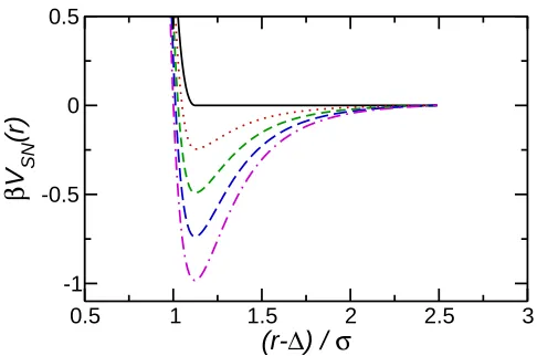
parameter ∆ is to shift the separation at which the interaction potential goes to infinity, giving the nanoparticle at non-zero size. It should be noted that this potential represents the nanoparticle as a single interaction and is similar to potentials used in previous studies15–17,21. This potential is a modification of the Lennard-Jones interaction to a particle of non-zero size. More sophisticated potentials explicitly representing the interaction of a superposition of pair potentials of atoms in a nanoparticle, may be found by integrating the Lennard-Jones potential over the volume of the nanoparticle36,37. Despite the difference in functional forms between the potential above (Eqn. 4) and that given in Ref36, they exhibit similar variation with nanoparticle-solvent separation, indicating that Eqn. 4 provides a good approximation to a superposition of pair interactions. Nanoparticles of radii 2.5σ ≤Rc ≤4σ were studied.
for the solvent define the usual set of reduced units; in particular the temperatureT∗ =ǫ/k B, mass m∗, and number density ρ∗ =N σ3/V.
The free energy profile or potential of mean force is determined using umbrella sampling32. The nanoparticle z-coordinate (zc) is constrained at a series of points zi using a harmonic
potential
Vi(zc) =
1
2ki(zc −zi) 2
(5)
where ki is the force constant (with βσ2k = 5−20). For each zi the (biased) probability
distribution Pi(zc) is determined and the final (unbiased) probability distribution P(z) is
determined using weighted histogram analysis38. For each value of ρ, R
c, and ǫ′ 2.5×10⁶
MD steps (including 0.5×10⁶ equilibration steps) were performed for each z
i. In order to
estimate errors in the free energy profiles, each of these simulation runs were divided into four subruns with the full analysis performed on these separately.
All simulations were performed using the Lammps simulation package39 in the NVT ensemble,with T∗ = 1. Temperature was controlled using a Nose-Hoover thermostat40. A timestep ofδt= 0.005t∗ (wheret∗ =pm∗σ2/ǫ) was used. In order to localise the interface in the centre of the simulation cell repulsive walls were placed in thez-direction, with periodic boundaries in the x and y directions. The average z-position of the interface is typically
|z¯inter| ≤0.004σ (with a typical standard deviation∼0.04σ), where the cell centre defined is
to be atz = 0. This allows the nanoparticle-interface separation to be approximated by the nanoparticlez-coordinate (zc). For comparison with continuum theory simulations without
nanoparticles were used to calculate the interfacial tension using the virial expression41
γAB =
Z dz
Pzz(z)−
Pxx(z) +Pyy(z)
2
(6)
where Pii(z) are the diagonal components of the pressure tensor. The values of γAB are
III. RESULTS
A. Effective nanoparticle-interface interaction
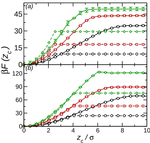
Shown in Fig. 2 are the free energy for the purely repulsive (ǫ′ = 0) nanoparticles. The free energy profiles have a minimum at zc = 0 and then rise to a maximum some distance from
the interface. As in previous work the range of the effective interaction is significantly larger than the particle radius caused by the broadening of the interface due to capillary waves. On increasing ρ the interaction range decreases due to the damping of the capillary wave amplitude with increase inγAB. In most cases the effective potential increases monotonically
towards the bulk value. For the Rc = 4σ atρ∗ = 0.69, however, a small barrier appears at
zc ≈6.1σ, presumably due to deformation of the interface by the nanoparticle, which would
be washed out due to interface fluctuations when the particle size is smaller or interfacial tension is lower. The height of this barrier, relative to the particle in bulk solvent is∼2kBT. Recent experimental studies42 on TEG-stabilised gold nanoparticles have also observed an activation barrier of approximately 2kBT (it should be noted that due to the differences between the simulated and experimental systems the agreement between the barrier heights in the two cases is likely to be fortuitous), which was attributed to electrostatic forces or rearrangement of attached chains. As the present system has neither of these this work demonstrates that such a barrier may also arise due to capillary effects29.
Also shown in Fig. 2 are the predicted effective potentials from the Pieranski approxima-tion. As the nanoparticle-solvent interaction is identical for both components, γAN = γBN
so Eqn. 1 reduces to
F(zc) =πγABz2c (7)
As in previous work this underestimates both the height of the barrier and also the inter-action range. The underestimation of the range arises due to its assumption of a sharp, flat interface (neglect of interface fluctuations). It is interesting to note that for the larger particles (Rc = 4σ) the simulation and Pieranski curves are in good agreement for the region
z ≤Rc.
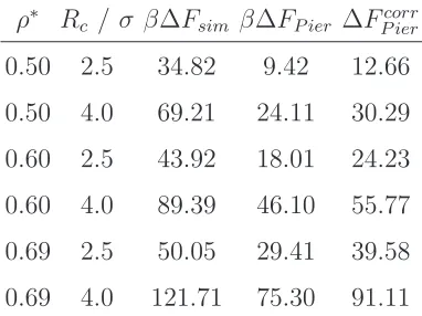
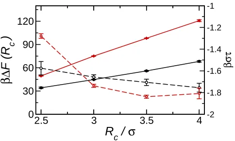
Shown in Fig. 3 are the detachment energies ∆F as a function ofRc. The values of ∆F are
a difference may be expected as the interfacial tension of the Widom-Rowlinson model is up to an order of magnitude lower to those obtained in this work. The present ∆F is similar to those recently obtained for polymer grafted nanoparticles20and from experimental measurements of gold nanoparticles42. The detachment energy (∆F) increases with particle radius. It is noticeable that this appears to scale approximately linearly with Rc rather
than quadratically as would be expected from the Pieranski approximation. This linear dependence may arise due to a significant line tension. The line tension is difficult to calculate, but it may be estimated from the difference between the detachment energies from simulation and Pieranski approximation15
τ =−∆Fsim −πR 2
cγAB
2πRc
. (8)
In all cases (Table 2) ∆Fsim > πR2cγAB, indicating that τ is negative, in agreement with
previous studies16,18. For ρ∗ = 0.50 τ decreases monotonically with R
c. For ρ∗ = 0.69,
however, τ decreases until Rc = 3.5σ and then remains approximately constant. On a
microscopic length scale, of course, the line tension should be interpreted with care44. This is partially due to the diffuse nature of the interface, which makes the identification of a three-phase contact line, hence estimating its length, difficult. Other effects, such as curvature corrections to the interfacial and surface tensions or terms related to the rigidity of the interface and stiffness of the contact line, may also effect the stability of particles at interfaces. The quantity τ appearing in Eqn. 8 may be regarded as a correction factor dependent that depends on the line tension and the role of line tension on the stability of nanoparticles at interfaces may only be fully determined through an independent calculation of the line tension45.
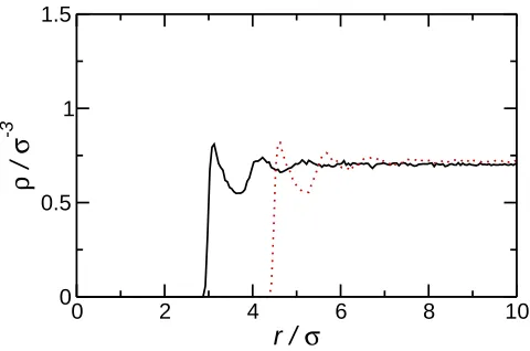
It should be noted that for small particles the radius Rc used in continuum theories (for
example in Eqn. 7) may not correspond to the radius of the particle. In particular due
to the finite size of the solvent particles the excluded volume due to the nanoparticle or, more importantly in the present case, the change in the interfacial area between the two solvent components, may be larger than would be expected from the value ofRc. The
effec-tive nanoparticle radius (Ref f
c )may be estimated from the solvent probability distribution
function (Fig. 4). From these Ref f
c = 2.9σ for Rc = 2.5σ and Ref fc = 4.4σ for Rc = 4σ.
between the detachment energies calculated from simulation and by Pieranski theory is the neglect of dispersion forces in the latter. While this may indeed lead longer ranged and stronger interactions between the nanoparticle and the interface, previous simulation work on purely repulsive hard sphere systems18 have shown a similar discrepancy, so dispersion forces are unlikely to be the primary reason for this. Additionally, while they are not ex-plicitly included in continuum models, dispersion forces are imex-plicitly included due to their contribution to interfacial and surface tensions in these theories.
B. Effect of attractive interactions
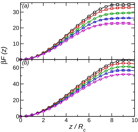
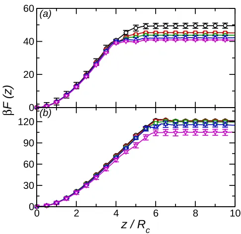
By changing ǫ′ the effect of attractive interactions between the nanoparticle and solvent particles may be examined. Note that as the nanoparticle-solvent interaction remains iden-tical for both solvent components the contact angle is constant (θ =π/2). Shown in Fig. 5 is the effective potential as a function of ǫ′ for ρ∗ = 0.50 (R
c = 2.5σ and 4σ). On increasingǫ′
the detachment energy decreases. This may be understood as the number of solvent particles close to the nanoparticle (hence in the attractive potential well) is lower at the interface, due to the depletion region between the two solvent components, than in the bulk solvent. At higher solvent density (Fig. 6) the behaviour ofF(z) on increasingǫ′ is the same. For the Rc = 4σ nanoparticle the small barrier that is present for ǫ′ = 0 disappears as ǫ′ increases.
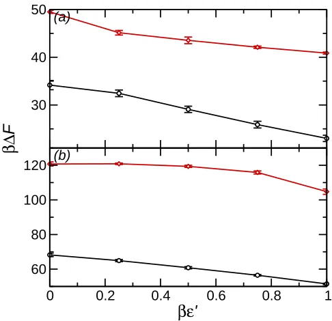
The variation in ∆F with ǫ′ for all ρ∗ studied is shown in Fig. 7. In all cases ∆F decreases with ǫ′. For ρ∗ = 0.50 the decrease with ǫ′ is approximately linear. On increasing ρ∗, however, the variation withǫ′is more complex. For theR
c = 4σnanoparticle atρ∗ = 0.69
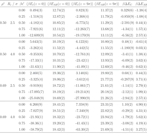
∆F is approximately constant for βǫ′ ≤ 0.25 before decreasing. In order to determine the contribution of the potential energy to ∆F the difference between the average nanoparticle-solvent interaction energies
hEci=
*Nsolvent X
i=1
VSN(|rc−ri|)
+
(9)
whereVSN(r) is given in Eqn. 4 and the angled brackets denote an average over a simulation
run, for nanoparticle constrained at zc = 0 (interface) and zc = 9σ (bulk) were calculated
(Tab. 3). Apart from βǫ′ = 0, ∆E
C = Ec(z = 9σ)− Ec(z = 0) is negative, indicating
with ǫ′ (for ρ∗ = 0.50 and R
c = 2.5σ, the difference between ∆F for βǫ′ = 1 and βǫ′ = 0
is approximately 11 kBT, while the difference between ∆EC is approximately 7 kBT). By contrast the difference between the average interaction energy (EAB) between the unlike
components
hEABi=
*NA X
i=1
NB X
j=1
VS(|ri−rj|)
+
(10)
for zc = 0 and zc = 9σ (∆EAB) shows no clear trend with ǫ′. This is expected as, at fixed
Rc, the change in interfacial area between the A and B components is the same for all ǫ′.
The remaining contribution to ∆F may arise from entropic effects due to changes in solvent structure around the nanoparticle, both at the interface and in bulk solvent.
C. Capillary waves
One of the underlying assumptions of continuum approximations such as Pieranski theory, are that the interface is sharp and flat. On the microscopic level the interface is broadened by bulk density fluctuations and thermal fluctuations in the interface position (capillary waves)46. Central to the microscopic description of interfaces is the notion of a local interface position h(r) (r = (x, y)), which is often more conveniently described through its
two-dimensional Fourier transform h(q). In particular, capillary wave theory (CWT) predicts
that at low q the mean-squared amplitudes of h(q) varies as47
h|h(q)|2i= 1 γβL2
xq2
(11)
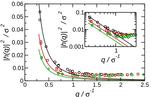
with q = |q|. Shown in Fig. 8 are the the plots of h|h(q)|2i for the three densities studied
in this work. At low-q h|h(q)|2i indeed displays the 1/q2 behaviour predicted by capillary
wave theory (although due to the finite size of the simulation box, only wavevectors with q >2π/Lx may be studied). At higher-qdeviations from CWT are seen, due to bulk density
fluctuations.
Recently Lehle and Oettel (LO) calculated a correction to the Pieranski expression us-ing a perturbative approach12. Within this approach the effective nanoparticle-interface interaction is given by
FLO(zc) =πγAB(zc −z0)2
1− τˆ ˆ
r3 0,eq 1 + ln ˆλc
1− rˆ0ˆτ,eq
where ˆτ =τ /(γABRc) is the reduced line tension,r0,eq =
p R2
c −zeq2 is the radius of the
con-tact line (for z =zeq), and ˆλc ≈1.12λc/r0,eq is the reduced capillary length. λc is effectively
the largest capillary wave in the system; for gravitational systemsλc =
p
γAB/(∆ρg) where
g is the acceleration due to gravity and ∆ρis the difference in mass density between the two phases, while in this caseλc =Lx (transverse box length).
Comparison between the effective potentials found from simulation and calculated using Eqns. 7 (Pieranski approximation) and 12 is shown in Fig. 9. For Rc = 2.5σ nanoparticle
the effective potential from simulation falls between the two theoretical predictions, with results from Eqn. 7 lying above and Eqn. 12 lying below the simulation curve. This may be understood as interface fluctuations lead to a more diffuse interface than assumed in Pieranski theory, so taking these into account leads to a softer interaction. For negative τ, as in this work, the effective potential from Eqn. 2 varies more rapidly than the effective potential from the Pieranski approximation18. ForR
c = 4σ nanoparticle both the Pieranski
and LO expressions give effective potentials that lie below the simulation results, with the potential from LO expression lying further from the simulation potential. In this case the poor performance of the LO equation is likely due to the assumption, made in its derivation that Rc ≪ λc is in valid (for the Rc = 4σ nanoparticle λc/Rc ≈ 4−5) and simulations of
larger systems would be needed to test its applicability.
The softening of the potential may be quantified through the (anharmonic) spring con-stant
k= d 2V dz2 z=0 , (13)
which in the case of the Pieranski8, AC, and LO approximations are12
kP ier = 2πγAB (14a)
kAC = 2πγAB 1−τ /ˆ rˆ03,eq
(14b)
kLO = 2πγAB
1−τ /ˆ rˆ3 0,eq
1 + log(ˆλ 1−τ /ˆ rˆ3 0,eq
) (14c)
(note that kP ier is independent of Rc). ksim is estimated from fitting a quadratic function
to the region z ≤ 2σ. The collected values of k are given in Table 4. For both ρ∗ = 0.50 and ρ∗ = 0.69 k
sim increases with Rc. The inclusion of line tension has only a small effect
onk, with the difference between kP ier and kAC decreasing asRc increases; the line tension
at low and high density. For ρ∗ = 0.50 it decreases very slightly with R
c. At ρ∗ = 0.69,
however, there is a substantial increase in kLO with Rc in agreement with simulation.
IV. CONCLUSIONS
In this paper molecular dynamics simulations have been used to calculate the effective interaction between a spherical nanoparticle and a liquid-liquid interface in a binary Lennard-Jones fluid. The effective interaction is qualitatively similar to that calculated previously for hard sphere systems18, although the detachment free energy is significantly larger (of the order of 10−100 kBT rather then 1−10kBT) due to the larger interfacial tension. As before comparison between simulation and the continuum Pieranski approximation shows that the latter underestimates the strength and range of the interaction. The difference between simulation and Pieranski theory may arise due to its neglect of line tension and microscopic effects such as capillary waves.
On including an attractive interaction between the nanoparticle and solvent particles the detachment energy of the nanoparticle decreases. This is as there are fewer close contacts between the nanoparticle and solvent particles when the nanoparticle is at the interface than when it is in bulk solvent. In the case studied here, when the contact angle θ = π/2 the detachment energy from Pieranski theory remains unchanged with the attraction strength. Calculation of the change in the average nanoparticle-solvent interaction energies for nanoparticles at the interface and in bulk solvent shows that this accounts for a significant proportion of ∆F. The remainder of the change in ∆F may arise from entropic contributions due to rearrangement of the particles around the nanoparticle.
One of the underlying assumptions of the Pieranski approximation (and other continuum theories) is that the interface is sharp and flat. This leads to an interaction potential that for small particles varies too rapidly near the interface. The inclusion of capillary waves into the effective potential leads to a noticeable softening of the potential, as shown by a large decrease in the spring constant.
nanoparticles, such as anisotropic or polymer tethered nanoparticles.
ACKNOWLEDGEMENTS
The author is grateful to Dr. Fernando Bresme for helpful comments. This work was funded by ERC, University of Warwick and the Leverhulme trust (ECF/2010/0254). Com-putational resources were provided by the Centre for Scientific Computing, University of Warwick.
1 F. Bresme and M. Oettel, J. Phys. Condens. Matt. 19, 413101/1 (2007). 2 W. H. Binder, Angew. Chemie Int. Ed. 44, 5172 (2005).
3 S. Cauvin, P. J. Colver, and S. A. F. Bon, Macromolecules 38, 7887 (2005). 4 P. S. Clegg, J. Phys. Condens. Matt.20, 113101/1 (2008).
5 M. B. Linder, Curr. Opin. Coll. Interf. Sci.14, 356 (2009).
6 J. T. Russell, Y. Lin, A. B¨oker, L. Su, P. Carl, H. Zettl, J. He, K. Sill, R. Tangirala, T. Emrick,
K. Littrell, P. Thiyagarajan, D. Cookson, A. Fery, Q. Wang, and T. P. Russell, Angew. Chem.
Int. Ed. 44, 2420 (2005).
7 P. Finkle, H. D. Draper, and J. H. Hildebrand, J. Amer. Chem. Soc. 45, 278 (1923). 8 P. Pieranski, Phys. Rev. Lett. 45, 569 (1980).
9 B. P. Binks and S. O. Lumsdon, Langmuir 16, 8622 (2000). 10 B. P. Binks and J. H. Clint, Langmuir 18, 1270 (2002).
11 R. Aveyard and J. H. Clint, Journal of the Chemical Society, Faraday Transactions 92, 85 (1996).
12 H. Lehle and M. Oettel, J. Phys. Condens. Matt. 20, 404224 (2008). 13 M. Oettel and S. Dietrich, Langmuir 24, 1425 (2008).
14 H. Lehle, M. Oettel, and S. Dietrich, EPL 75, 174 (2006). 15 F. Bresme and N. Quirke, Phys. Rev. Lett. 80, 3791 (1998). 16 F. Bresme and N. Quirke, J. Chem. Phys. 110, 3536 (1999).
18 D. L. Cheung and S. A. F. Bon, Physical Review Letters 102, 066103/1 (2009). 19 D. L. Cheung and S. A. F. Bon, Soft Matter 5, 3969 (2009).
20 R. J. K. Udayana Ranatunga, R. J. B. Kalescky, C.-c. Chiu, and S. O. Nielsen, J. Phys. Chem.
C 114, 12151 (2010).
21 F. Bresme, H. Lehle, and M. Oettel, J. Chem. Phys. 130, 214711/1 (2009). 22 L. L. Dai, R. Sharma, and W. C.-Y., Langmuir 21, 2641 (2005).
23 Y. Song, M. Luo, and L. L. Dai, Langmuir 26, 5 (2010). 24 D. L. Cheung, Chem. Phys. Lett. 495, 55 (2010).
25 P. Hopkins, A. J. Archer, and R. Evans, J. Chem. Phys. 131, 124704 (2009). 26 M. Zeng, J. Mi, and C. Zhong, Phys. Chem. Chem. Phys.13, 3932 (2011). 27 B. Widom and J. S. Rowlinson, J. Chem. Phys. 52, 1670 (1970).
28 M. Oettel, A. Domingeuz, and S. Dietrich, Phys. Rev. E 71, 051401 (2005). 29 Y.-M. Ban, R. Tasseff, and D. Kopelevich, Mol. Sim. 37, 525 (2011).
30 M. E. Flatte, A. A. Kornyshev, and M. Urbakh, J. Phys. Condens. Matt. 20, 073102 (2008). 31 F. Wang and D. Landau, Phys. Rev. Lett. 86, 2050 (2001).
32 G. Torrie and J. Valleau, J. Comp. Phys. 23, 187 (1977). 33 S. Park and K. Schulten, J. Chem. Phys.120, 5946 (2004). 34 A. Laio and F. L. Gervasio, Rep. Prog. Phys. 71, 126601 (2008).
35 E. Darve, D. Rodr´ıguez-G´omez, and A. Pohorille, J. Chem. Phys.128, 144120 (2008). 36 R. Everaers and M. Ejtehadi, Phys. Rev. E 67, 041710 (2003).
37 P. J. in’t Veld, M. K. Petersen, and G. S. Grest, Phys. Rev. E79, 021401 (2009).
38 S. Kumar, J. M. Rosenberg, D. Bouzida, R. H. Swendsen, and P. A. Kollman, J. Comp. Chem.
13, 1011 (1992).
39 S. Plimpton, J. Comp. Phys. 117, 1 (1995),http://lammps.sandia.gov. 40 W. G. Hoover, Phys. Rev. A 31, 1695 (1985).
41 J. H. Irving and J. G. Kirkwood, J. Chem. Phys. 18, 817 (1950).
42 K. Du, E. Glogowski, T. Emrick, T. P. Russell, and A. D. Dinsmore, Langmuir26, 12518 (2010). 43 B. P. Binks, Curr. Opin. Coll. Inter. Sci. 7, 21 (2002).
44 L. Schimmele, M. Napiorkowski, and S. Dietrich, J. Chem. Phys. 127, 164715 (2007). 45 Y. Djikaev, J. Chem. Phys. 123, 184704 (2005).
47 S. A. Safran, Statistical thermodynamics of surfaces, interfaces, and membranes (Persus,
Table 1.
Lateral box lengths (note Lz = 2Lx), pressure, and interfacial tensions for the studied
systems.
ρ∗ L
x / σ βσ3P βσ2γAB
Table 2.
Detachment free energies calculated from simulation (∆Fsim) and using the Pieranski
approximation (Eqn. 7). β∆FP ier refers to detachment energy calculated using Rc, while
β∆Fcorr
P ier denotes detachment energy calculated using corrected Rc found from the solvent
density distribution.
ρ∗ R
c / σ β∆Fsim β∆FP ier ∆FP iercorr
Table 3.
Average nanoparticle (Ec) and A-B interaction (EAB) energies for zc = 0 andzc = 9σ.
Statistical errors in the final digit, estimated from the standard error of 50000 measurements given in parenthesis.
ρ∗ R
c /σ βǫ′ hβEc(z = 0)i hβEAB(z = 0)i hβEc(z = 9σ)i hβEAB(z = 9σ)i β∆EC β∆EAB
0.50 2.5
0.00 0.494(3) 12.74(2) 0.823(3) 11.37(2) 0.329(6) -1.38(4) 0.25 -1.518(3) 12.87(2) -2.368(4) 11.79(2) -0.850(9) -1.08(4) 0.50 -4.182(4) 10.85(2) -6.773(5) 11.29(2) -2.591(9) 0.44(4) 0.75 -7.921(6) 12.11(2) -12.263(7) 13.68(2) -4.34(1) 1.57(4) 1.00 -12.609(9) 10.54(2) -19.170(9) 13.11(2) -6.56(2) 2.57(4)
0.50 4.0
0.00 5.643(5) 10.19(2) 6.122(6) 10.80(2) 0.48(1) -0.61(4) 0.25 -3.262(4) 11.52(2) -4.442(5) 11.55(2) -1.180(9) 0.03(4) 0.50 -9.353(6) 10.70(2) -12.761(8) 12.09(2) -3.41(1) 1.38(4) 0.75 -17.33(1) 10.31(2) -23.42(1) 13.93(2) -6.09(2) 3.62(4) 1.00 -31.63(1) 11.90(2) -41.09(1) 12.60(2) -9.46(2) 0.62(4)
0.69 2.5
0.00 2.460(5) 19.36(2) 3.140(6) 19.80(2) 0.68(1) 0.44(3) 0.25 -3.325(4) 18.06(2) -3.612(4) 21.77(2) -0.287(9) 3.71(4) 0.50 -9.919(6) 18.72(2) -11.061(7) 21.61(2) -1.14(1) 2.79(4) 0.75 -17.095(7) 18.19(2) -19.214(8) 20.18(2) -2.12(1) 1.99(4) 1.00 -25.048(9) 18.69(2) -27.990(9) 21.26(2) -2.94(2) 2.57(4)
0.69 4.0
Table 4.
Line tensions and spring constants for ǫ′ = 0 nanoparticle. Numbers in parenthesis give errors in final digits.
ρ∗ R
c /σ βστ βσ2ksim βσ2kP ier βσ2kAC βσ2kLO
0.50
2.5 -1.58 2.068 3.014 3.27(1) 2.130(2) 3.0 -1.66 2.341 3.014 3.143(2) 2.1246(4) 3.5 -1.71 2.478 3.014 3.086(1) 2.1100(3) 4.0 -1.76 2.799 3.014 3.057(1) 2.1085(2)
0.69
FIGURE CAPTIONS
Fig. 1. Nanoparticle-solvent interaction potentials (Eqn. 4) withβǫ′ = 0 (solid, black),βǫ′ = 0.25 (dotted, red), βǫ′ = 0.50 (dashed, green), βǫ′ = 0.75 (long dashed, blue), and βǫ′ = 1 (dot-dashed, magenta). Solvent-solvent interaction (Eqn. 3) corresponds to ∆ = 0 and βǫ′ = 1 andβǫ′ = 0 for like (A-A and B-B) and unlike (A-B) interactions respectively.
Fig. 2. (a) Free energy profile forRc = 2.5σ nanoparticle (ǫ′ = 0) at solvent densityρ∗ = 0.50
(circles, black), ρ∗ = 0.60 (squares, red), and ρ∗ = 0.69 (diamonds, green). Solid line shows simulation results, dashed lines Pieranski approximation. (b) Free energy profiles forRc = 4.0σ nanoparticle (ǫ′ = 0). Symbols as in (a).
Fig. 3. Detachment energy and line tension against Rc for ρ∗ = 0.50 (circles, black) and
ρ∗ = 0.69. Circles denote ρ∗ = 0.50, diamonds ρ∗ = 0.69, ∆F denoted by filled symbols (solid lines) and τ denoted by open symbols (dashed lines).
Fig. 4. Solvent density distributions around Rc = 2.5σ (solid line) and Rc = 4.0σ (dotted
line) nanoparticles (βǫ′ = 0) at solvent density ρ∗ = 0.69.
Fig. 5. (a) Free energy profile forRc = 2.5σ nanoparticle at solvent densityρ∗ = 0.50. Circles
(black) denotesβǫ′ = 0, squares (red)βǫ′ = 0.25, diamonds (green)βǫ′ = 0.5, triangles (blue) βǫ′ = 0.75, and inverted triangles (magenta) βǫ′ = 1. (b) Free energy profile for Rc = 4σ nanoparticle at solvent density ρ∗ = 0.50. Symbols as in (a).
Fig. 6. (a) Free energy profile forRc = 2.5σ nanoparticle at solvent densityρ∗ = 0.69. Circles
(black) denotesβǫ′ = 0, squares (red)βǫ′ = 0.25, diamonds (green)βǫ′ = 0.5, triangles (blue) βǫ′ = 0.75, and inverted triangles (magenta) βǫ′ = 1. (b) Free energy profile for Rc = 4σ nanoparticle at solvent density ρ∗ = 0.69. Symbols as in (a).
Fig. 7. (a) Detachment energy against ǫ′ for R
c = 2.5σ nanoparticle at solvent densities
ρ∗ = 0.50 (circles, black) and ρ∗ = 0.69 (diamonds, red). (b) Detachment energy againstǫ′ forR
c = 2.5σ nanoparticle. Symbols as in (a).
Fig. 8. Mean-squared Fourier components of the interface position h|h(q)|2i for ρ∗ = 0.50
predictions of capillary wave theory. The inset shows the same data on a log-log plot.
Fig. 9. (a) Effective nanoparticle-interface interaction forRc = 2.5σnanoparticle atρ∗ = 0.50
Fig. 1
D. L. Cheung
Journal of Chemical Physics
0.5 1 1.5 2 2.5 3
(r-∆) / σ
-1 -0.5 0 0.5
β
V SN
[image:23.595.71.314.289.450.2]Fig. 2
D. L. Cheung
Journal of Chemical Physics
0 15 30 45
β
F (z
c
)
0 2 4 6 8 10
z c / σ
0 30 60 90 120
(a)
[image:24.595.71.312.289.518.2]Fig. 3
D. L. Cheung
Journal of Chemical Physics
2.5 3 3.5 4
R
c / σ
0 30 60 90 120
β∆
F (R
c
)
-2 -1.8 -1.6 -1.4 -1.2 -1
[image:25.595.72.314.290.435.2]Fig. 4
D. L. Cheung
Journal of Chemical Physics
0 2 4 6 8 10
r / σ
0 0.5 1 1.5
ρ
/
σ
[image:26.595.73.313.290.449.2]Fig. 5
D. L. Cheung
Journal of Chemical Physics
0 10 20 30
β
F (z)
0 2 4 6 8 10
z / Rc
0 20 40 60
(a)
[image:27.595.71.313.289.521.2]Fig. 6
D. L. Cheung
Journal of Chemical Physics
0 20 40 60
β
F (z)
0 2 4 6 8 10
z / Rc
0 30 60 90 120
(a)
[image:28.595.70.313.288.524.2]Fig. 7
D. L. Cheung
Journal of Chemical Physics
30 40 50
β∆
F
0 0.2 0.4 0.6 0.8 1
βε’
60 80 100 120
(a)
[image:29.595.71.314.290.525.2]Fig. 8
D. L. Cheung
Journal of Chemical Physics
0 0.5 1 1.5 2 2.5
q / σ-1
0 0.01 0.02 0.03 0.04 0.05 0.06
|h(q)|
2
/
σ
2
1
q / σ-1
0.001 0.01 0.1
|h(q)|
2
/
σ
[image:30.595.72.316.290.447.2]Fig. 9
D. L. Cheung
Journal of Chemical Physics
0 0.5 1 1.5 2 2.5
0 10 20 30
β
F(z)
0 1 2 3 4
z / σ
0 25 50 75
β
F(z)
(a)
[image:31.595.71.314.287.541.2]