Randomised techniques in combinatorial algorithmics

(1)

University of Warwick institutional repository:

http://go.warwick.ac.uk/wrap

A Thesis Submitted for the Degree of PhD at the University of Warwick

http://go.warwick.ac.uk/wrap/61092

This thesis is made available online and is protected by original copyright.

Please scroll down to view the document itself.

(2)

THE LIBRARY Tel: +44 1203 523523 Fax: +44 1203 524211

AUTHOR:

Michele A. A. Zito

DEGREE:

Ph.D.

TITLE:

Randomised Techniques in Combinatorial Algorithmics

DATE OF DEPOSIT: 16 JULY, 1999

I agree that this thesis shall be available in accordance with the regulations

govern-ing the University of Warwick theses.

I agree that the summary of this thesis may be submitted for publication.

I agree that the thesis may be photocopied (single copies for study purposes only).

Theses with no restriction on photocopying will also be made available to the British Library for microfilming. The British Library may supply copies to individuals or libraries. subject to a statement from them that the copy is supplied for non-publishing purposes. All copies supplied by the British Library will carry the following statement:

“Attention is drawn to the fact that the copyright of this thesis rests with its author. This copy of the thesis has been supplied on the condition that anyone who consults it is understood to recognise that its copyright rests with its author and that no quotation from the thesis and no information derived from it may be published without the author’s written consent.”

AUTHOR’S SIGNATURE:

. . . .

USER’S DECLARATION

1. I undertake not to quote or make use of any information from this thesis

with-out making acknowledgement to the author.

2. I further undertake to allow no-one else to use this thesis while it is in my care.

DATE

SIGNATURE

ADDRESS

. . . .

(3)

Randomised Techniques in Combinatorial Algorithmics

by

Michele A. A. Zito

Thesis

Submitted to the University of Warwick

for the degree of

Doctor of Philosophy

Department of Computer Science

(4)

List of Figures

1.1 Approcessor PRAM . . . 7

1.2 The 64 distinct labelled graphs on 4 vertices. . . 16

1.3 The 11 distinct unlabelled graphs on 4 vertices. . . 17

1.4 Examples of random graphs . . . 19

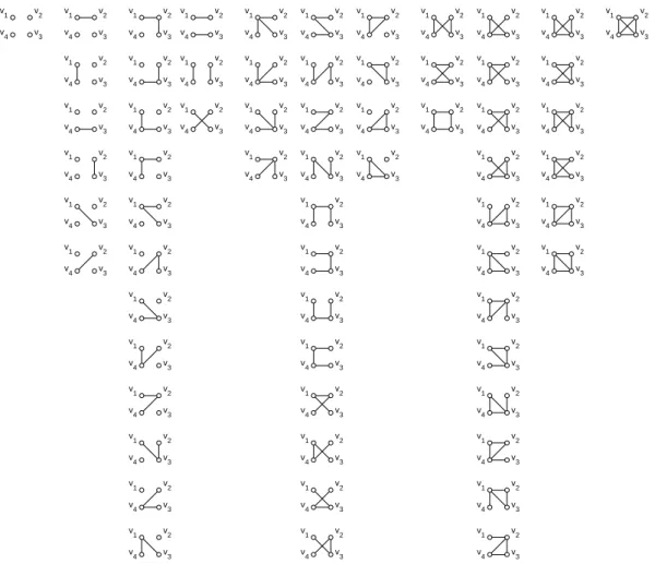
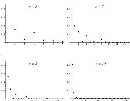
2.1 Probability distributions on conjugacy classes forn=5;7;8;10. . . 29

2.2 Example of set family. . . 33

2.3 Integer partitions of 8 in different representations. . . 36

2.4 Distribution of different orbits forn=4. . . 45

2.5 Values of G after step (2). . . 53

3.1 A legal 3-colouring (left) and a maximal 3-colouring (right). . . 69

3.2 Legal edges for a vertexv. . . 71

3.3 Partition of the parameter space used to upper boundE(X ℄ ). . . 83

3.4 Graph off 1 (x (r);y (r)). . . 87

3.5 Locating the best value of. . . 89

4.1 Possible Vertex Covers . . . 94

4.2 Gadget replacing a vertex of degree one in a bipartite graph. . . 97

4.3 A(1;3)-graph and its 2-padding. . . 98

4.4 A cubic graph with small maximal matching and large induced matching. . . 104

4.5 Ad-regular graph with small maximal matching and large induced matching. . . . 105

4.6 A cubic graph with small maximal induced matching. . . 106

4.7 Gadgets for a vertexv i 2V(G). . . 111

4.8 Gadget replacing a vertex of degree one. . . 112

4.9 Gadget replacing a vertex of degree two. . . 113

4.10 Possible ways to define the matching inG 0 given the one inG. . . 113

(7)

4.12 Filling an empty gadget, special cases. . . 115

4.13 Possible relationships between pairs of split independent sets . . . 121

(8)

Acknowledgments

Although my work in Theoretical Computer Science has been mainly a solitary walk through

Dis-crete Mathematics and Computational Complexity Theory, I would like to thank the many people

that joined my walk from time to time or that helped my progress, first in Warwick University and

then in the University of Liverpool.

First and foremost I would like to thank Alan Gibbons, my supervisor for his presence, his

trust in me and his constant support. He has always been much more optimistic about my work than

myself and he has often given me the strength to go on. Also I thank Mike Paterson and Martin Dyer

for their careful reading of my thesis. Their comments and suggestions have contributed to improve

the quality of my work.

I would also like to thank all the people that I met at Warwick. I feel particularly indebted

to S. Muthukhrishnan (Muthu). His company, scientific, and social advice was a pleasure during the

many days and evenings that we spent together at Warwick.

My thanks go also to all the people in the Department of Computer Science, at the

Univer-sity of Liverpool, especially Paul Dunne, Ken Chan and all the technical staff, for their friendship

and support. Thanks to William (Billy) Duckworth, my office colleague during my staying in

Liv-erpool (at least until he decided that the other hemisphere is more interesting than this one), for

keeping me interested in spanners and teaching me the exact difference between “tree”, “three” and

“free”! It was a great pleasure for me to work with him.

I thank the ‘Universit´a di Bari’ in Italy for giving me the cultural means and the financial

support to start my scientific journey. I am particularly grateful to Prof. Salvatore Caporaso, who

introduced me to the Theory of Computation. I valued his conversations, the many arguments and

the useful discussions we had. I also thank Nicola Galesi for the time we spent together, the work

we did and the rock&roll music we played.

Finally, last but not least, I feel deeply grateful to my parents and my wife, for their constant

love and support.

(9)

Declarations

This thesis is submitted to the University of Warwick in support of my application for admission to

the degree of Doctor of Philosophy. No part of it has been submitted in support of an application for

another degree or qualification of this or any other institution of learning. Parts of the thesis appeared

in the following refereed papers in which my own work was that of a full pro-rata contributor:

M. Zito, I. Pu, M. Amos, and A. Gibbons. RNC Algorithms for the Uniform Generation of

Combinatorial Structures. Proceedings of the 7th ACM-SIAM Annual Symposium on Discrete

Algorithms, pp. 429–437, 1996.

P. E. Dunne and M. Zito. An Improved Upper Bound on the Non-3-colourability Threshold.

Information Processing Letters, 65:17–23, 1998.

M. Zito. Induced Matchings In Regular Graphs and Trees. Proceedings of the 25th

Interna-tional Workshop on Graph-Theoretic Concepts in Computer Science, 1999. Lecture Notes in

Computer Science, vol 1665, Springer Verlag.

M. Zito. Small Maximal Matchings in Random Graphs. Submitted LATIN’2000: Theoretical

Informatics.

Unrefereed papers were also presented as follows:

M. Zito, I. Pu, A. Gibbons. Uniform Parallel Generation of Combinatorial Structures. 11th

British Colloquium on Theoretical Computer Science, Swansea, April 1995. Bulletin of the

European Association of Theoretical Computer Science, 58, 1996.

I. Pu, M. Zito, M. Amos, A. Gibbons. RNC Algorithms for the Uniform Generations of Paths

and Trees in Graphs. 11th British Colloquium on Theoretical Computer Science, Swansea,

April 1995. Bulletin of the European Association of Theoretical Computer Science, 58, 1996.

P. E. Dunne and M. Zito. On the 3-Colourability Threshold. 13th British Colloquium on

Theoretical Computer Science, Sheffield, 1997. Bulletin of the European Association of

The-oretical Computer Science, 64, 1998.

(10)

Abstract

Probabilistic techniques are becoming more and more important in Computer Science. Some of them are useful for the analysis of algorithms. The aim of this thesis is to describe and develop applications of these techniques.

We first look at the problem of generating a graph uniformly at random from the set of all unlabelled graphs withnvertices, by means of efficient parallel algorithms. Our model of parallel

computation is the well-known parallel random access machine (PRAM). The algorithms presented here are among the first parallel algorithms for random generation of combinatorial structures. We present two different parallel algorithms for the uniform generation of unlabelled graphs. The algo-rithms run inO(log

2

n)time with high probability on an EREW PRAM usingO(n 2

)processors.

Combinatorial and algorithmic notions of approximation are another important thread in this thesis. We look at possible ways of approximating the parameters that describe the phase tran-sitional behaviour (similar in some sense to the transition in Physics between solid and liquid state) of two important computational problems: that of deciding whether a graph is colourable using only three colours so that no two adjacent vertices receive the same colour, and that of deciding whether a propositional boolean formula in conjunctive normal form with clauses containing at most three literals is satisfiable. A specific notion of maximal solution and, for the second problem, the use of a probabilistic model called the (young) coupon collector allows us to improve the best known results for these problems.

(11)

Chapter 1

Introduction

This chapter provides, in the first section, the algorithmic context of this thesis. The remainder of

the chapter describes essential technical preliminaries for all subsequent chapters.

1.1 Algorithmic Background

Probabilistic techniques are becoming more and more important in Computer Science. Probabilistic

paradigms can be grouped in two main classes: those concerned with the construction of randomised

algorithms (under some reasonable model of computation) and those involved in the analysis of

al-gorithms. Among the first, some have acquired wide popularity. Random sampling is often used

to guess a solution in problems for which a large set of candidate solutions provably exists. A

re-cent beautiful application of this technique is in the problem of computing the minimum spanning

tree of a graph [KKT95]. Random re-ordering can be used to improve the performances of sorting

algorithms [Knu73]. Montecarlo simulation of suitably defined Markov chains or (some other

ran-domised dynamic process) finds wider and wider applications in generation and counting problems

[DFK91] as well as in algorithmic analysis [FS96]. Finally what is called sometimes control

ran-domisation (loosely speaking different algorithms or sub-routines are run on the particular problem

instance depending on some random choices) is exploited to devise good hashing algorithms and

for the complementary pattern matching problem [KR87]. In all cases the main advantages of the

specific algorithmic solution over more traditional deterministic approaches are simplicity and good

performance improvement It could be argued that this is achieved at the price of a more involved

(12)

traditional techniques anyway, this does not seem a major problem.

As mentioned at the beginning there is also another class of probabilistic paradigms.

Al-though not directly related to algorithmic design, their use helps in understanding the combinatorial

structure of several computational problems. Normally the set of all inputs for a specific problem is

viewed as a probability space (see Section 1.2.3 for a formal definition of this concept) and this fact is

exploited in either the performance analysis of specific algorithms or the understanding of structural

properties of combinatorial problems. In the former case, sometimes called input randomisation

[Bol85], the advantage is that the usual “case approach” is abandoned and therefore

worst-case instances only marginally influence the complexity of the different algorithmic solutions. In

the latter case, sometimes, the probabilistic approach enables us to understand the behaviour of few

parameters characterising the specific problem [ASE92].

The aim of this thesis is to describe and develop a few applications of several probabilistic

techniques related to the second type of paradigm described above. The usual assumption about

input randomisation is that input instances can indeed be generated with the desired distribution.

In some cases this is an important problem in its own right. For example it is still an important

open problem to find an efficient algorithm for generating a planar graph uniformly at random

[HP73, DVW96, Sch97]. Several techniques have been developed to build sequential algorithms for

generating combinatorial structures according to some predefined probability distribution [NW78].

In Chapter 2 we look at the issues involved in finding parallel algorithms for sampling combinatorial

objects uniformly at random. In some cases trivial parallelisation of a sequential algorithm solves

the problem quite efficiently. In some others the nature of the problem seems to prevent efficient

solutions. The focus of this work is on “unlabelled” structures. All relevant definitions are given in

Chapter 1.2 and 2. Loosely speaking the aim is to sample an object in a given set, disregarding a

number of possible symmetries. For instance, if we were to sample the result of throwing two dice,

we might be only interested in the sum of the two individual outcomes, not their ordered values.

In this case the order among the two outcomes is irrelevant. In Chapter 2 we will study similar

problems in the context of graph theory.

Combinatorial and algorithmic notions of approximation are another important thread in

this thesis. One of the generation algorithms described in Chapter 2 outputs a graph with a

prob-ability distribution that, in some sense, only approximates the uniform one. In Chapter 3 we look

at possible ways of approximating the parameters that describe the phase transitional behaviour

(13)

computational problems: that of deciding whether a graph is colourable using only three colours

so that no two adjacent vertices receive the same colour, and that of deciding whether a

proposi-tional boolean formula in conjunctive normal form with clauses containing at most three literals is

satisfiable. A specific notion of maximal solution and, for the second problem, the use of a

proba-bilistic model called (young) coupon collector allow us to improve the best known results for these

problems.

Chapter 4 is even more about approximation, but the final part of it will describe a

num-ber of results obtained through the use of a numnum-ber of probabilistic techniques. We look at two

graph theoretic problems. A graph is given, as a collection of nodes and edges joining them, and

we are interested in finding a set of disjoint edges satisfying some additional constraints. The goal

in each case is to find an “optimal” set according to some criterion that is part of the specific

prob-lem definition. We first study the computational complexity of these probprob-lems and the algorithmic

approximability of the optimal solutions, in particular classes of graphs. Then we make some

as-sumptions about the input distribution, we study the expected structure of these matchings and we

derive improved approximation results on several models of random graphs (see Section 1.2.5 for

the formal definitions).

The thesis is mainly self-contained. All concepts used in it are defined. Original definitions

are numbered whereas, normally, well-known concepts are introduced in a less formal way and

nor-mally referenced. All original results are proved in full details. All non-original results are clearly

stated and their proof is normally either sketched or the reader is referred to an appropriate

biblio-graphic reference. Chapter 2 contains some general definitions from the branches of mathematics

and computability that are related to this thesis; the reader familiar with the specific field should

be able to skip Chapter 2. However, to avoid conceptual discontinuities, a few specific technical

concepts and results are introduced in the relevant chapters.

1.2 Technical Preliminaries

We recall some basic terminology and well-known results in the different areas of Computer Science

and Mathematics which will be used later on. This section contains all those background definitions

and results which are particularly useful in more than one of the following chapters, or simply too

long to be put in the specific chapter, without distracting the reader’s attention.

(14)

function on real numbers, for everyy 2IR[f 1;+1g,f(x)!y(or simplyf !ywhen the

independent variable is clear from the context) is a shorthand for

lim x!1

f(x)=y

Also, the reader should be familiar with sequential computational models like Turing machines or

Random Access Machines [AHU74] and basic complexity theoretic definitions [GJ79, BDG88].

Asymptotic notations likeO(n 2

),o(1),(n),!(2 n

)and(n)will denote function classes but we

will normally writef =(n)(instead off 2 (n)) with the intended meaning that there exists

a constant such thatf(n) n fornsufficiently large. The reader is referred to Section 2.1

in Cormen, Leiserson and Rivest [CLR90], for more formal definitions. In particular, given two

functionsf andgon integers, we will writef gand we will say thatf is asymptotic togif the

ratiof(n)=g(n)!1(the concept can be extended to functions on real numbers).

This section’s content can be subdivided into two parts. The first two sections describe

con-cepts from Computability Theory and Computational Complexity. The remaining sections present

some relevant definitions and results from different areas of Mathematics.

More specifically, in Section 1.2.1 we recall some elementary definitions related to

com-putational problems that will be used throughout this thesis. Section 1.2.2 defines the models of

parallel computation which will be used in Chapter 2. Also the relevant complexity measures and

complexity classes are defined. Section 1.2.3 introduces the basic terminology related to

Probabil-ity Theory. Section 1.2.4 describes the relevant concepts in graph theory. Section 1.2.5 provides

a glimpse into the beautiful and by now well established theory of random graphs. We describe

several models of random graphs, each providing a different framework for the analysis of

combi-natorial and algorithmic properties of graphs. Finally Section 1.2.6 introduces all basic definitions

and results in group and action theory that will be needed later, especially in Chapter 2.

1.2.1 Problems

Many computational problems can be viewed as the seeking of partial information about a relation

(see [BDG88, Chapter 1] or [BC91]). More specifically supposeis a finite alphabet and that

problem instances and solutions are encoded as strings over. A relationSOL

defines

an association between problem instances and solutions. For everyx2

the setSOL (x)contains

all they 2

that encode a solution associated withx, with the implicit convention that ifxdoes

not encode a problem instance thenSOL (x) =;. For everyx 2

(15)

(the encoding)x. Notice incidentally that ifS is a set,jSjwill be used, in the usual sense, as the

cardinality ofS. In this setting a decision problem is described by the relationSOLand a question

which has a yes/no answer in terms ofSOL [BDG88, p. 11]. Ifx 2

, a decision problem

(also known as existence problem) answers the following question: is there ay 2

such that

y 2 SOL(x)? Ifx;y 2

are given, another decision problem (which will be referred to as the

membership problem) answers the question: doesybelong toSOL (x)?

There is a natural correspondence between a decision problemQand the setQof instances

that have a “yes” answer. Thus no strong distinction betweenQandQwill be kept: the “name” of

the decision problem will also denote the set of instances with a solution. Notice thatQ

so

the words language or property will also be used as qualifiers.

Several other types of problems are definable in this setting. Informally, ifx 2

is (the

encoding of) a problem instance then

1. a construction problem (or search problem) aims at exhibiting ay 2

such that(x;y) 2 SOL;

2. an optimisation problem, given a cost function (x;y), aims at finding the y 2

with

(x;y)2SOLsuch that(x;y)is maximised (respectively minimised);

3. a uniform generation problem, aims at generating a wordy 2

satisfying(x;y) 2 SOL

such that allyinSOL (x)come up equally often;

4. a counting problem, aims at finding the number of elements inSOL (x).

Example. In what follows we recall, in a rather informal way, a number of definitions related

to boolean algebra. The reader is referred to [BDG88, Chapter 1] or [Dun88] for a more formal

treatment of the subject.

A boolean formula is an expression like

(x 3

;x 12

;x 25

;x 34

;x 70

)= df

(x 25

^x 12

)_:(:x 70

_(:x 3

^x 34

))

built up from the elementsx

iof a countable set

X of propositional variables, a finite set of

connec-tives (usually including^,_and:) and the brackets.

If variables are assigned values over a binary set of truth-values denoted byV = f0;1g

and connectives are interpreted in the usual way as operations onV then each formula represents

a function onV. It is evident that under this interpretation the formula(x 3

;x 12

;x 25

;x 34

;x 70

(16)

equivalent to(x 1

;x 2

;x 3

;x 4

;x 5

)obtained by replacingx 3with

x 1,

x 12with

x

2and so on. Thus,

without loss of generality, a formula onndifferent variables can be regarded as containing exactly

the variablesx 1

;:::;x n. Let

X n

=fx 1

;:::;x n

g. Sometimes notation(~x )will be used instead

of(x 1

;x 2

;:::;x n

).

^

1 1 1

1 0 0

0 0 1

0 0 0

_

1 1 1

1 1 0

0 1 1

0 0 0

:

1 0

0 1

Any function : X n

! V is called annvariable-assignment (or simply a

truth-assignment). Notationfgwill be used for the truth-value ofafter each variablex

i has been

replaced by(x i

)and the tables above (called truth-tables) have been used to find the truth-value

of conjunctions, disjunctions or negations of truth-values. Since truth-values are nothing but binary

digits, the set of alln-variable-truth-assignments will normally be denoted byf0;1g n

.

The formula is said to be in conjunctive normal form (CNF for short) if it is in the form

C 1

^C 2

:::^C m

where each clauseC

iis the disjunction of some variables or negation of variables (expressions like x

ior :x

i are called literals). Every boolean formula can be transformed by purely algebraic rules

into a CNF formula (see for example [BDG88, p. 17–18]). A CNF formulais ink-CNF if the

maximum number of literals forming a clause isk.

Everyk-CNF formulae can be encoded over the finite alphabet = f^;_;:;(;);0;1g

(e.g. variablex

i is encoded by the binary representation of

i). In this setting,k-SAT is the well

known NP-complete problem [GJ79] of deciding whether ak-CNFis satisfiable, i.e. whether

there exists an assignmentof values inV to all variables insuch that the value ofunder this

assignment is one.

Combinatorial structures associated with computational problems can be characterised by a

number of parameters, describing specific features of the problem instances. For example ak-CNF

formula is built on somenvariables,mclauses and each clause has at mostkliterals. A graph (see

Section 1.2.4 for relevant definitions) might havenvertices,medges, maximum degree. In most

cases it will be possible to define two functions on natural numbers, the order and the size.I n

(17)

The relationships between different parameters characterising the instances of two specific

problems will be the object of the work described in Chapter 3. We conclude this section with a

remark and a couple of useful definitions.

It is worth noticing that there might be no relationship between these parameters and the

length of the encoding of the instances of a particular problem. For instance the natural encoding of

ak-CNF formula of order (i.e. number of variables)nand size (i.e. number of clauses)mdescribed

in the example above has length at mostkmlogn.

A setQ

is a monotone increasing property (respectively monotone decreasing

prop-erty) with respect to a partial order<

Qif for every fixed n x2I

n

\Q;y2I n

;x< Q

y(respectivelyy< Q

x))y2Q

A setQ

is a convex property if for everyx;y;z 2 I n

x < Q

y < Q

zandx;z 2 Qimply y2Q.

1.2.2 Parallel Computational Complexity

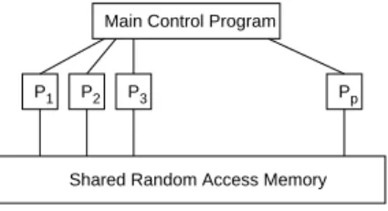
The algorithms described in Chapter 2 are designed for an idealised model of parallel computation

called (see [GR88], for example) parallel random access machine (PRAM).

P_p

Shared Random Access Memory

P₁ P₂ P₃

Main Control Program

Figure 1.1: Approcessor PRAM

There arep processors working synchronously and communicating through a common

random-access memory. Each processor is a sequential random access machine (or RAM for short)

in the spirit of [CR73]. The set of arithmetic operations available to each processor includes

ad-dition, subtraction, multiplication and division between arbitrary length integers at unit cost. Each

RAM is also augmented with a facility to generate random numbers. The expressions rand(0;1)is

a call to a function returning a random real number between 0 and 1. Tuples of values (also called

records) will be used occasionally. For example, following the most standard notations,x:date is

the identifier for the variable associated with the field “date” of the record structurex. Ordinal

(18)

field variables as well as whole record variables are allowed. Constant tuples will be represented by

lists of value. For example(4;1;3:14;3)is a constant four-tuple. Constant time direct and indirect

indexing allow us to handle (multidimensional) arrays of integers or real numbers. For exampleA[i℄

is thei-th element of an arrayA,A[i:j℄is the portion ofAbetween indexiand indexj, defined if jiand withA[i:i℄=A[i℄. The expressionA[i;℄denotes the row vector formed by all elements

in rowi. In what follows the terms array and list will be used interchangeably.

In a single computation step each processor can perform any arithmetic operation on the

proper number of operands stored in the shared memory. Notationa b+is a shorthand for the

sequence

feth(R 1

;b);feth(R 2

;);R 3

R 1

+R 2

;store(a;R 3

);

including three memory transfer operations and one arithmetic manipulation. However given the

asymptotic nature of the complexity results proved in Chapter 2,a b+will be counted as

a single step. OperandsR 1,

R 2 and

R

3are registers local to each processor: each processor has

available a constant number of them (the exact value of this constant being irrelevant). All the

algorithms do not use shared access to the same memory location in a single time step. A PRAM

enforcing this constraint is called Exclusive Read Exclusive Write PRAM (or EREW PRAM). Other

models allowing some degree of concurrent access are the Concurrent Read Exclusive Write PRAM

(or CREW PRAM) and the Concurrent Read Concurrent Write PRAM (or CRCW PRAM).

A PRAM algorithm will normally be specified as a sequence of instructions in a

PASCAL-like pseudo-code. The most important syntactic constructs are listed below.

Assignments such asa b+are the simplest instructions.

Programs will contain typical control structures like if-then-else conditionals, for and while

loops. In particular when similar tasks need to be performed on different data a parallel for

loop statement might be used. The syntax will be as follows

for allx2X in parallel do instructions

Indentation will show nested instructions.

The complexity measures we use are (parallel) running time and number of processors,

nor-mally expressed in asymptotic notation and as a function of the input length. By efficient algorithms

we mean algorithms that run in polylogarithmic (i.e. O(log k

n)for some constantk) time in the

(19)

NC. A PRAM algorithm, in particular, is said to be optimal (see [GR88]) if the product of its

par-allel running timet(n)with the number of processors usedp(n)is within a constant factor of the

computation time of the fastest existing sequential algorithm. The quantityw(n)=t(n)p(n)is

called work.

Function and procedure names will often be used as macros. In particular the following

pre-defined subroutines are assumed.

1. A function copying inO(logn)time usingO(n=logn)processors an elementxacross all

positions of an array ofnelements. The syntax will be copy(x;n)and the result will be an

array ofnelements all equal tox.

2. A function computing an associative operation on a list ofnelements in a certain domain, in O(logn)time usingO(n=logn)processors. The function will have as parameters the list,

its sizen, the operation to be performed and will return a value of the appropriate type. The

correct syntax for the function computing the sum of thenelements of a listLis tree(L;n;+).

3. If+is an associative operation over some domainDandL[1℄;:::;L[n℄is an array of elements

ofD the prefix sums problem is to compute thenprefix sumsS[i℄ = P

i j=1

L[j℄fori = 1;:::;n. The algorithms in Chapter 2 will make use of a function prefix, computing the prefix

sums of a list ofnelements in parallel (this is also known as parallel prefix computation).

If Lis a list of nelements and is the integer multiplication, then the instruction R

prefix(L;n;)is carried out inO(logn)parallel steps usingO(n=logn)processors, ifnis

the number of element of the listL. After this instruction it will beR [i℄= Q

i j=1

L[j℄.

The following definition (essentially from [Joh90]) captures the class of PRAM algorithms

which will be of interest in Chapter 2.

Definition 1 A search problem belongs to the class RNC if there exists a randomised PRAM

algo-rithmAwhose running time is polylogarithmic which uses a polynomial number of processors and

such that

1. ifSOL(x)6=;thenAoutputsy2SOL (x)with probability more than 1/2;

2. ifSOL(x)=;then the output ofAis undefined.

Indeed, in all cases, the parallel algorithms in this thesis will satisfy a stronger condition.

(20)

by an inverse polynomial function. In all such cases we say that the algorithms succeed with high

probability.

Sometimes it is convenient to slow down part of a parallel algorithm in order to achieve

optimal work over the whole algorithm. Consider a computation that can be done intparallel steps

withx

i primitive operations at step

i. Trivial parallel implementation will run intsteps onm = maxx

iprocessors. If we have

p<mprocessors theith step will be simulated indx i

=pex i

=p+1

time and so the total parallel time is no more than

P t i=1

x i

=p+t. This is known as Brent’s scheduling

principle [Bre74]. This is assuming that processor allocation is not a problem: for specific problems

we may need to provide the processor allocation scheme explicitly (i.e. redesigning the algorithm

to work usingpprocessors). Sometimes this principle can be used to find the number of processors

which gives optimal work. For examples all library functions above have optimal work whenever

p(n)=O(n=logn). Of course reducing the number of processors will slow down the computation.

So if the parallel prefix operation is run on a list of n elements usingn=log 5

nprocessors the

resulting algorithm runs inO(log 5

n)parallels steps.

1.2.3 Probability

Many of the results in this thesis are probabilistic. In this section some terminology and general

results are given.

Following [GS92], a probability space is a triple(;;Pr), whereis a set called a sample

space,= fE: E gis the set of events andPris a non-negative real valued measure on

withPr[℄=1. The elements ofare particular events called elementary events. Unless otherwise

statedwill be a finite set andwill be the set of all subsets of. For everyE2the probability

of the eventE,Pr[E℄= df

P !2E

Pr[!℄.

Theorem 1 The probabilities assigned to the elements of a sample spacesatisfy the following

properties (for everyE;F 2):

1. Pr[E℄0.

2. (Monotonicity) IfEFthenPr[E℄Pr[F℄.

3. Pr[E[F℄=Pr[E℄+Pr[F℄ Pr[E\F℄.

4. Pr[

(21)

Theorem 2 (Total probability) IfE 1

;:::;E

nis a partition of

withE i

2for alliandE 2

thenPr[E℄= P

n i=1

Pr[E\E i

℄.

Proof. Immediate from Theorem 1.3 since the eventsE\E

iare all disjoint.

2 Pr[EjF℄will denote the probability of the eventE given that the eventF has happened.

IfPr[F℄ >0, we definePr[EjF℄ = df

Pr[E\F℄=Pr[F℄. A sequence of eventsE

iare mutually

independent ifPr[E 1

\:::E n

℄ = Q

n i=1

Pr[E i

℄. Mutual independence between pairs of events is

called pairwise independence.

Example. Let=fa;b;;dgwithPr[a℄=qandPr[b℄=Pr[℄=Pr[d℄=p. LetE

1

=fa;bg, E

2

=fa;gandE 3

=fa;dg. Pr[E i

℄ =p+qandPr[E 1

\E 2

\E 3

℄ =Pr[fag℄ =q. Solving q=(p+q)

3

with the constraint3p+q=1we get Pr[E

1 \E

2 \E

3

℄=Pr[E 1

℄Pr[E 2

℄Pr[E 3

℄

forp=(3 p

3)=4andq=(3 p

3 5)=4. On the other handPr[E i

jE j

℄ =q=(p+q)6=Pr[E i

℄.

Similarly sample spaces can be built in which it is possible to construct events that are pairwise

independent but not mutually independent.

A real valued random variableXon a probability space(;;Pr)is a function fromto

the set of real numbers such that for every real numberxthe setf!2: X(!)xg2. The

distribution function of a random variableXis the functionF :IR![0;1℄withF(x)=Pr[X x℄.

Moments. Ifhis any real-valued function on the set of real numbersIRthen the expectation of h(x)is

E(h(X))= df

X

h(x)Pr[X=x℄

In particular the mean of a random variableX, usually denoted by, isE(X)and thek-th moment of XisE(X

k

)(of course, ifis not finite, these quantities might not exist). Thek-th binomial moment

ofXisE( X

k

)whereas thek-th factorial moment ofXisE k

(X)= df

E(X(X 1):::(X k+1)).

It follows thatE k

(X)=k!E( X

k

).

Theorem 3 IfX =

P X

ithen

E(X)= P

E(X i

).

This result, known as linearity of expectation, (the proof follows immediately from the definition of

(22)

value ofXis the sum of a number of very simple random variablesX

ithen the mean of

Xis easily

defined in terms of the means of theX i.

The variance ofX, usually denoted by 2

, is defined byVar(X) = df

E((X ) 2

) = E(X

2 )

2

.

Theorem 4 IfX =

P X

iand the X

iare pairwise independent then

Var(X)= P

Var(X i

).

Theorem 5 IfX is a positive random variable thenPr[X℄E(X

k )=

k

for every>0and

integerk>0.

Proof. By definitionE(X

k )

P x

x k

Pr[X=x℄. Ifxthen the sum above is lower bounded

by k

Pr[X℄and the result follows. 2

Theorem 5 has many useful special cases, depending on the choices ofandk.

Theorem 6 (Markov inequality)Pr[X>0℄E(X).

Theorem 7 (Chebyshev inequality)Pr[jX E(X)j℄

2

.

An important use of Chebyshev inequality is in proving that a positive random variable takes

a value larger than zero with “high” probability (this property will be used repeatedly for example

in Chapter 4).

Corollary 1 IfX 0thenPr[X=0℄Var(X)=E(X)

2

.

Proof.Pr[X=0℄Pr[jX E(X)j℄if==. 2

So assuming that a natural numberncan be associated as a parameter with the elements

of the sample space under consideration, and thatE(X)andVar(X)are thus functions of n, if lim

n!1

E(X) = 1 andVar(X) = o(E(X) 2

) then the last corollary implies thatPr[X = 0℄

becomes smaller and smaller as a function ofn.

Distributions. We now briefly review the discrete probability distributions that will be used in

later chapters. The discrete uniform distribution on a finite sample spacecontainingnelements is

defined by

Pr[! i

℄= 1 n

8i2f1;:::;ng

and in this case we say that!

iis generated uniformly at random. The random variable

X : ! f1;:::;ngdefined byX(!

i

(23)

are distributed uniformly over). Using the following simple identities, which can be easily proved

by induction onn, n X i=1

i=

n(n+1) 2 n X i=1 i 2 =

n(n+1)(2n+1) 6

it is possible to derive

E(X)= 1 n n X i=1 i= 1 n

n(n+1) 2

= n+1

2 Var(X) = 1 n n X i=1 i

n+1 2 2 = 1 n " n X i=1 i 2 n X i=1

i(n+1)+ n X i=1

(n+1) 4 2 # = 1 n n X i=1 i 2 n X i=1 i

n+1 2

+

(n+1) 4 2 = 1 n n X i=1 i 2

n(n+1) 2 + n 2 1 4 = 1 n n X i=1 i 2

n+1 2

2 =

(n+1)(2n+1) 6

n+1

2 2 = n 2 1 12

IfX :!f0;1gandPr[X=1℄=pthenXis called a 0–1-random variable or random

indicator. 0–1-random variables model an important class of random processes called Bernoulli

trials. During one of these trials an experiment is performed which succeeds with a certain positive

probabilityp. In particular from now on we will always abbreviate Pr[X = 1℄ byPr[X℄ and Pr[X=0℄byPr[X℄. We have

E(X)=0(1 p)+1p=p Var(X)=(0 p)

2

(1 p)+(1 p) 2

p=(1 p)(p 2

+p p 2

)=p(1 p)

Random indicators have many applications in probability. For example they can be used to estimate

the variance of a random variable.

Theorem 8 IfXcan be decomposed in the sum ofnnot necessarily independent random indicators

then

1. Var(X)2 P fi;jg Pr[X i ^X j

℄+E(X)where the sum is over all 2-sets onf1;:::;ng.

2. Var(X)E 2

(24)

Proof. It follows from the definition thatVar(X) E(X 2

). For every real numberx > 0we

can writex 2

= x+2 x 2

. HenceE(X 2

) = E(X)+2E( X

2

). IfX = P i X i then X 2 is the

number of ways in which two differentX

ican assume the value one, disregarding the ordering. So E( X 2 )= P fi;jg E(fX i ;X j g)= P fi;jg Pr[X i ^X j

℄over allfi;jgf1;:::;ng.

The second inequality is trivial sinceE 2

(X)=2E( X

2

). 2

The proof of Theorem 8 gives a combinatorial meaning toE( X

2

)in terms of the random

indicatorsX i. If

X = P n i=1 X iwhere X

iare random indicators also the

k-moment and thek-th

factorial moment ofXhave an interpretation in terms of theX i.

E(X 2

)is the sum over all pairs of

(not necessarily distinct)iandjofPr[X i

^X j

℄whereE 2

(X)is the sum over all ordered pairs of

distinctiandjofPr[X i ^X j ℄. IfX i are

n independent random indicators with common success probability equal top

thenX = P

n i=1

X

ihas binomial distribution with parameters

nandp. Simple calculations (using

Theorem 3 and 4) imply

E(X)=np Var(X)=np(1 p)

If a sequence of identical independent random experiments is performed with common

success probability equal topthen the random variableY

1counting the number of trials up to the

first success has geometric distribution with parameterp. Pr[Y 1

=k℄=p(1 p) k 1

hence using

the binomial theorem and some easy properties of power series

E(Y 1

)=1=p Var(Y 1

)= 1 p

p 2

In the same setting as aboveY

k counting the number of trial up to the

k-th success has the

Pascal distribution (or negative binomial distribution).Pr[Y k

=n℄= n 1 k 1 p k (1 p) n k . Since

each trial is independentY k = P k j=1 Y j 1

where theY j 1

have a geometric distribution. Hence by

Theorem 3 and Theorem 4 and the results for the geometric distribution we have

E(Y k

)=k=p Var(Y k

)=

k(1 p) p

2

Improved Tail Inequalities. The beauty of Theorem 5 resides in the fact the only assumption

made onX is on the existence ofE(X k

). If more accurate information is available it is

possi-ble to improve considerably the quality of the results. The following Theorem states a couple of

(25)

Theorem 9 Letn2INand letp 1

;:::;p n

2IRwith0p i

1,i=1;:::;n. Putp=(1=n) p i

andm = npand let X 1

;:::;X

n be independent 0-1 random variables with Pr(X

i ) = p

i ; i = 1;:::;n. LetS =

P X

i. Then

Pr(S(1+)m)e

2 m=3

; 01

and

Pr(S(1 )m)e

2 m=2

; 01:

In most cases the Chernoff bounds stated above will be used on a sequence ofnindependent

iden-tically distributed 0-1 random variables. Under these assumptions,Shas binomial distribution and

some improved bounds are possible (see [Bol85, Ch. I]).

1.2.4 Graphs

Most of the graph-theoretic terminology will be taken from [Har69] and [Bol79]. A (simple

undi-rected) graphG= (V;E)is a pair consisting of a finite nonempty setV =V(G)of vertices (or

nodes or points) and a collectionE=E(G)of distinct subsets ofV each consisting of two elements

called edges (or lines). Ife=fu;vg2Ethen the verticesuandvare adjacent, vertexuand the

whole edgeeare incident (or else we say that ubelongs toe, sometimes using the set-theoretic

notationu2e). Also iff =fv;wg2Etheneandf are incident. IfF E(G)thenV(F)is the

set of vertices incident to somee2F. For everyU V(G),N(U)will denote the set of vertices

adjacent to somev2U and not belonging toU. IfU =fvgwe writeN(v)instead ofN(fvg). If U;W V then cut(U;V)is the set of edges having one endpoint inU and the other inW.

The degree of a vertexvis defined asdeg G

v= df

jN(v)j. The minimum (resp. maximum)

degree ofGis Æ = Æ(G) = min v2V

deg G

v (resp. = (G) = max v2V

deg G

v). For all i2f0;:::;n 1gletV

i

(G)=fv2V :deg G

v=ig. A multiset is a collection of objects in which

a single object can appear several time. A multigraph is a pairH =(U;E)in whichU is the set of

vertices andEis a multiset of edges. Ifeappearsx e

>1times inEthen each of its occurrences is

a parallel edge. The skeleton of a multigraphH =(U;E)is a graphGwithV(G)=U andE(G)

containing a single copy of every parallel edge inH plus all thee 2 Ewithx e

= 1. A graph is

directed if the edges are ordered pairs. Round brackets will enclose vertices belonging to a directed

edge.

A graph is labelled if its vertices are distinguished from one another by names. Figure 1.2

(26)

v v v v 1 2 3 4 v v v v 1 2 3 4 v v v v 1 2 3 4 v v v v 1 2 3 4 v v v v 1 2 3 4 v v v v 1 2 3 4 v v v v 1 2 3 4 v v v v 1 2 3 4 v v v v 1 2 3 4 v v v v 1 2 3 4 v v v v 1 2 3 4 v v v v 1 2 3 4 v v v v 1 2 3 4 v v v v 1 2 3 4 v v v v 1 2 3 4 v v v v 1 2 3 4 v v v v 1 2 3 4 v v v v 1 2 3 4 v v v v 1 2 3 4 v v v v 1 2 3 4 v v v v 1 2 3 4 v v v v 1 2 3 4 v v v v 1 2 3 4 v v v v 1 2 3 4 v v v v 1 2 3 4 v v v v 1 2 3 4 v v v v 1 2 3 4 v v v v 1 2 3 4 v v v v 1 2 3 4 v v v v 1 2 3 4 v v v v 1 2 3 4 v v v v 1 2 3 4 v v v v 1 2 3 4 v v v v 1 2 3 4 v v v v 1 2 3 4 v v v v 1 2 3 4 v v v v 1 2 3 4 v v v v 1 2 3 4 v v v v 1 2 3 4 v v v v 1 2 3 4 v v v v 1 2 3 4 v v v v 1 2 3 4 v v v v 1 2 3 4 v v v v 1 2 3 4 v v v v 1 2 3 4 v v v v 1 2 3 4 v v v v 1 2 3 4 v v v v 1 2 3 4 v v v v 1 2 3 4 v v v v 1 2 3 4 v v v v 1 2 3 4 v v v v 1 2 3 4 v v v v 1 2 3 4 v v v v 1 2 3 4 v v v v 1 2 3 4 v v v v 1 2 3 4 v v v v 1 2 3 4 v v v v 1 2 3 4 v v v v 1 2 3 4 v v v v 1 2 3 4 v v v v 1 2 3 4 v v v v 1 2 3 4 v v v v 1 2 3 4 v v v v 1 2 3 4

Figure 1.2: The 64 distinct labelled graphs on 4 vertices.

labelling of their vertices, their topological structure is the same. More formally, two graphsG 1

andG

2are isomorphic if there is a one-to-one correspondence between their labels which preserves

adjacencies. A graph is unlabelled if it is considered disregarding all possible labelling of its vertices

that preserve adjacencies. Figure 1.3 shows the eleven unlabelled graphs on four vertices.

A graph is completely determined by either its adjacencies or its incidences. This

informa-tion can be conveniently stated in matrix form. The adjacency matrix of a labelled undirected (resp.

directed) graphG = (V;E)withnvertices, is annnmatrixAsuch that, for all v i

;v j

2 V, A

i;j

=1ifv

iis adjacent to v

j(resp. if (v

i ;v

j

)2E) andA i;j

=0otherwise.

A subgraph ofG = (V;E)is a graphH = (W;F)withW V andF E. H is a

spanning subgraph ifW =V and it is an induced subgraph if wheneveru;v2W withfu;vg2E

thenfu;vg2 F. IfW V(G)we will denote byG[W℄the induced subgraph ofGwith vertex

setW. K

nis the complete simple graph on

nvertices. It hasn(n 1)=2edges. Every graph onn

(27)

A graphG = (V;E)is bipartite ifV can be partitioned in two setsV 1and

V

2 such that

every line ofGjoins a vertex inV

1 with a vertex in V

2. K

n 1

;n 2

is the complete bipartite graph

onn =n 1

+n

2 vertices. A graph is planar if it can be drawn on the plane so that no two edges

intersect.

IfGis a graph andv 2V thenG vis the graph obtained fromGby removingvand all

edges incident to it; ifv62V thenG+v=(V [v;E). Ife=fu;vg2EthenG e=(V;Enfeg)

andG+e=(V [fu;vg;E[e). These operations extend naturally to sets of vertices and edges.

Figure 1.3: The 11 distinct unlabelled graphs on 4 vertices.

A path in a graphG=(V;E)is an ordered sequence of vertices formed by a starting vertex vfollowed by a path whose starting vertex belongs toN(v). The path is simple if all vertices in the

sequence are distinct. The length of a pathP = (v 1

;:::;v k

)isk 1. A cycle is a simple path P=(v

1 ;:::;v

k

)such thatv 1

=v

k. A single vertex is a cycle of length zero. Since

v62N(v)there

is no cycle of length one. An edgefu;vg2 Ebelongs to a pathP =(v 1

;:::;v k

)if there exists i2 f1;:::;k 1gsuch thatfu;vg=fv

i ;v

i+1

g. Two verticesuandv in a graph are connected

if there is a pathP =(v 1

;:::;v k

)such thatfu;vg=fv 1

;v k

g. The distancedst G

(u;v)between

them is the length of a shortest path between them. The subscriptGwill be omitted when clear from

the context. A connected component is a subgraph whose vertex set isU V, such that allu;v2U

are connected and nov2V nU is connected to someu2U.

1.2.5 Random Graphs

LetG n;m

be the set of all (labelled and undirected) graphs withnvertices andmedges. IfN = n 2

andG n

= S

N m=0

G n;m

thenjG n;m

j = N m

andjG n

j =2 N

. Informally, a random graph is a pair

formed by an elementGofG n

along with a non-negative real valuep

Gsuch that P

G2G n

p G

=1.

In other words random graphs are elements of a probability space associated withG n

, called the

random graph model. There are several random graph models. In most cases the set of events is the

set of all subsets ofG n

and the definition is completed by giving a probability to eachG2G n

. If

is a random graph model we will writeG2 to mean thatPr[G℄is defined according to the given

model.

(28)

nvertices andmedges and assigning to all other graphs probability zero. For eachm=0;1;:::;N, G(n;m)has

N m

elements that occur with the same probability N m

1

. Sometimes the alternative

notationG(K n

;m)is used instead ofG(n;m), whereK

nis called the base graph since the elements

of the sample space are all subgraphs of the complete graph. Variants ofG(n;m)are thus obtained

by changing the base graph. For example the sample space ofG(K n;n

;m)is the set of all bipartite

graphs onn+nvertices andmedges. This is made into a probability space by giving the same

probability to all such graphs.

In the modelG(n;p)(sometimes denoted byG(K n

;p)) we have0<p<1and the model

consists of all graphs withnlabelled vertices in which edges are chosen independently and with

probabilityp. In other words ifG 2 G(n;p) andjE(G)j = mthenPr[G℄ = p m

(1 p) N m

.

A variant ofG(n;p)is G(K n

;(p i;j

))in which edgefi;jgis selected to be part of the graph or

not with probabilityp

i;j. So for example G(K

n;n

;p), whose sample space is the set of bipartite

graphs onn+nvertices in which each edge is present with probabilityp, is indeed an instance of G(K

2n ;(p

i;j )).

To avoid undesired inconsistencies it is important that under fairly general assumptions

results obtained on one model translate to results in another model. A propertyQholds almost

always (or a.a.), for almost all graphs or almost everywhere (a.e.) iflim n!1

Pr[G2Q℄=1. The

following theorem, reported in [Bol85, Ch.II], relatesG(n;p)andG(n;m).

Theorem 10 (i) LetQbe any property and suppose thatlim

n!1

p(1 p)N = +1. Then the

following two assertions are equivalent.

1. Almost every graph inG(n;p)hasQ.

2. Givenx>0and>0, ifnis sufficiently large, there arel(1 )2x p

p(1 p)Nintegers M

1 ;:::;M

lwith pN x

p

p(1 p)N <M 1

<M 2

<:::<M l

<pN+x p

p(1 p)N

such thatPr Mi

[Q℄>1 for everyi=1;:::;l.

(ii) IfQis a convex property andlim n!1

p(1 p)N =+1, then almost every graph in G(n;p)hasQ, whereM =bpN+x

p

p(1 p)N.

(iii) IfQis a property and0<p=M=N<1then Pr

M

[Q℄Pr p

[Q℄e 1=6M

p

2p(1 p)N 3 p

MPr p

(29)

The success of a random graph model depends on many factors. From a practical point of

view the model must be reasonable in terms of real world problems and it must be computationally

easy to generate graphs according to the specific distribution assigned by the model. From the

theoretical point of view the choice of one model over another depends on the specific problem at

hand and it is often a matter of trading-off the simplicity of combinatorial calculations performed

under the assumption that a given graph was sampled according to a certain model, for the tightness

of the desired results.G(n;m)often gives sharper results but it is sometimes more difficult to handle

thanG(n;p). In Chapter 3 a slightly different model will be used which keeps the good features of G(n;m)and is easier to analyse. LetM

n;m

be the set of all (labelled and undirected) multigraphs

onnvertices and medges; let M n

= S

1 m=0

M n;m

. M(n;m)is the probability space whose

sample space is the set of pairs(M;)whereM 2 M n;m

and is a permutation ofmobjects

(see Section 1.2.6 for further details on permutation groups) giving an ordering on themedges of M. The probability measure on the sample space assigns the same probabilityN

m

to all elements

ofM n;m

S

m. Strictly speaking,

M(n;m)is a random multigraph model. Figure 1.4 shows

1

2

3 4 5

6 ₇

1

2

3 4 5

7 6

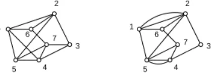
Figure 1.4: Examples of random graphs

a graph on 7 vertices and 13 edges and a multigraph with the same number of vertices and edges.

In particular the multigraph shown on the right corresponds tom!elements of the sample space of M(n;m), one for each possible ordering. The model is somehow intermediate betweenG(n;m)

and the uniform model or multigraph process model as defined in [JKŁP93] in whichmordered

pairs of (not necessarily distinct) elements of[n℄=f1;2;:::;ngare sampled.

The practical significance ofM(n;m)is supported by the very simple process which

en-ables us to generate an element in this space: formtimes select uniformly at random an element in [n℄

(2)

, the set of unordered pairs of integers in[n℄=f1;:::;ng.

Again a result that relates properties ofM(n;m)to those ofG(n;m)is needed. The

fol-lowing suffices for the purposes of Chapter 3.

Theorem 11 LetXandY be two random variables defined respectively onG(n;m)andM(n;m).

IfX(G)=Y(G)for everyG2G n;m

\M n;m

(30)

Proof.

E(X) = X G2G

n;m X(G)

m!(N m)! N!

X G2G

n;m X(G)

m! (N m)

m =

X G2G

n;m X(G)

m! N

m

1 m N

m

Ifm=nsinceN =n(n 1)=2we have

1 m N

m e

2

n n 1

which is asymptotic toe

2

. Hence

E(X)O(1) X G2G

n;m X(G)

m! N

m

For every simple graphGwithmedges there are exactlym!elements of(G;) 2 M n;m

S m

SinceX(G)=Y(G)for everyG2G n;m

\M n;m

we can writeE(X)O(1)E(Y). 2

1.2.6 Group Theory

Most of the definitions and the results in this section are taken from [Rot65].

Basic Definitions. A group is an ordered pair(G;)whereGis a set andis a binary operation

onGsatisfying the following properties:

g1 g

1 (g

2 g

3 )=(g

1 g

2 )g

3for all g

1 ;g

2 ;g

3 2G.

g2 There existsid2G(the identity) such thatgid=g=idgfor allg2G.

g3 For allg 1

2Gthere existsg 2

2G(the inverse ofg

1, often denoted by g

1 1

) such thatg 1

g 2

= id=g

2 g

1.

IfXis a nonempty set, a permutation ofX is a bijective functiongonX. LetS

X denote

the set of permutations onX. Although most of the definitions are general, in all our subsequent

discussionXwill be the set[n℄.

There are many ways to represent permutations. We will normally use the cycle notation

defined as follows:

(31)

(2) Join the point labelledito the point labelledjby an edge with an arrow

pointing towardsjifg(i)=j. (This will form a number of cycles).

(3) Write down a list(i 1

;i 2

;:::;i k

)for each cycle formed in step (2).

(4) Remove all lists formed by a single element.

So for exampleg 2 S 6 with

g(1) = 3, g(2) = 2,g(3) = 4g(4) = 1,g(5) = 6and g(6)=5will be represented as(134)(56). It is possible to associate a unique multisetf1:k

1 ;2: k

2

;:::;n:k n

g(sometimes represented symbolically asx k

1 1

x k

2 2

:::x kn n

or simply[k 1

;k 2

;:::;k n

℄)

to every permutationg2S

ndescribing its cycle structure (or cycle type): ghask

icycles of length i. In particulark

1is the number of elements of

[n℄that are fixed byg, i.e. such thatg(i) =i. If g(i)6=iwe say thatgmovesi.

Ifg 1

;g 2

2S Xthen

g 1

Æg

2is a new function on

Xsuch that(g 1

Æg 2

)(x)= df

g 1

(g 2

(x)). It

is easy to verify thatg 1

Æg 2

2S

X. The pair (S

X

;Æ)is indeed a group called the symmetric group

onX.S

nwill denote both the set S

[n℄and the group (S

[n℄ ;Æ).

Subgroups and Lagrange Theorem. If(G;)is a group, a nonempty subsetHofGis a subgroup

of(G;)if

sg1 g

1 g

2

2Hfor allg 1

;g 2

2H.

sg2 The identity of(G;)belongs toH.

sg3 g

1

2Hfor allg2H.

Theorem 12 IfH is a subgroup of a groupGthen there existsm2IN +

such thatjGj=mjHj.

Proof. (Sketch, see [Rot65] for details) GivenHandg2G, define the setgH =fgh:h2Hg.

It follows from g1-g3 and sg1-sg3 that

1. jgHj=jHjfor allg2G.

2. Ifg 1

6=g 2

2Gthen eitherg 1

H =g 2

H org 1

H\g 2

H =;.

3. For allg 1

2Gthere existsg 2

2Gsuch thatg 1

2g 2

H.

So there exists anmsuch thatG=g 1

H[:::[g m

H and the setsg i

H form a partition ofG. 2

The study of permutation groups is strictly related to the study of graphs because a graph

(32)

Definition 2 [HP73] Given a graphG =(V;E)the collection of all permutationsg 2 S V such

thatfu;vg2 Eif and only iffg(u);g(v)g 2Efor allu;v 2V is the automorphism group ofG

and is denoted by Aut(G).

The structure and the properties of the automorphism group of a graph are of particular

importance in the study of unlabelled graphs and isomorphisms between labelled graphs.

Action Theory. A group(G;)acts on a setif there is a function (called action):G!

such that

1. id=for each2.

2. g 1

(g 2

)=(g 1

g 2

)for allg 1

;g 2

2Gand2.

The action ofGoninduces an equivalence relationon(if and only if=gfor some g2G). The equivalence classes are called orbits. For eachg2G, defineFix(g)=f2:g= gand conversely for each2define the stabilizer ofto be the set

=fg2G:g=g.

Lemma 1 is a subgroup of

G.

In particularS

ncan be acting on itself:

fg=fÆgÆf 1

. In this caseis called conjugacy

relation and the orbits are called conjugacy classes. In what followsCwill denote a conjugacy class

inS n.

Theorem 13 Conjugacy classes inS

nare formed by all permutations with the same cycle type.

Proof. Ifg =:::(:::ij:::):::thenhÆgÆh 1

has the same effect of applyinghto the elements

ofghencegandhÆgÆh 1

have the same cycle type. Letf andgbelong to the same conjugacy

class. Thenf =hÆgÆh 1

for someh2S

n. But this implies that

fhas the same cycle type ofg.

Conversely iffandghave the same cycle type, align the two cycle notations, definehand

it is easy to prove thatf andgare conjugate. 2

Thus the number of different conjugacy classes is the same as the number of different cycles

types. From now on, a conjugacy classCwill be identified with the decomposition ofndefining the

cycle type of the permutations inC. The following result is well known (see for example [Kri86]).

Theorem 14 The number of permutations with cycle type[k

1 ;:::;k

n ℄is

n! Q

n i=1

(i k

ik i

!)

(33)

Proof. Given the form of the cycle notation

( )( ):::( ) | {z }

k 1

( ; )( ; ):::( ; ) | {z }

k 2

:::( ; ;:::; ) | {z }

x | {z }

k x

it is possible to count the number of ways to fill it.

There aren!ways to fill thenplaces. The firstk

1unary cycles can be arranged in k

1 !ways. Thek

2 cycles of length 2 can be arranged in k

2

! ways times for each of thek

2 cycles the

possible ways to start (two). Sok 2

!2 k

2 overall. Similarly fork

i, there are

iways to start one of thei-cycles. Hencek i

!i ki

ways to putik i

chosen items in cycles of lengthi.

2

The following theorem states a couple of well known results which will be useful.

Theorem 15 LetGbe a finite group acting on a set6=;.

1. (Orbit-Stabilizer Theorem) For each orbit!,jf(g;):2!\Fix(g)gj=jGj.

2. (Fr¨obenius-Burnside Lemma) The number of orbits is

m= 1 jGj

X 2 j

j=

1 jGj

X g2G

jFix(g)j:

Proof. For each orbit! the elements off(g;) : 2 !\Fix(g)g are pairs withg 2

and 2!. There arej

jj!jof these pairs. The first result follows from Theorem 12 applied to

since there is a bijectionbetween! and the collectiong i : if

2 !then =gfor some g2G; define()=g

.

The first part of the second result follows from the first result. Assume there are! 1

;:::;! m

different orbits. Summing over all2!

iwe have X

2!i j!

i jj

j=

X 2!i

jGj

and from this

X 2! i

j! i

jj

j=j! i

(34)

and finally, simplifying on both sides

X 2!i j

j=jGj

Finally, adding over all orbits

m X i=1

X 2!i j

j=mjGj

To understand the second equality observe that the sum on the left in the expression above is counting

pairs(g;)for 2 andg 2

. This is equivalent to count pairs

(g;) forg 2 G and 2 Fix(G). Hence

m X i=1

X 2! i

j

j= X g2G

jFix(g)j

2

Pair Group and Combinatorial Results. LetS

(2)

n be the permutation group on the set of

un-ordered pairs of numbers in[n℄. Every permutationg2S

ninduces a permutation g

2S

(2) n defined

byg

(fi;jg)=fg(i);g(j)g.

Theorem 16 Letf;g2CS

nand assume the cycle type of Cis[k

1 ;:::;k

n ℄. Then

1. f

g

;

2. jFix(g)j=2 q(C)

whereq(C)is the number of cycles ofg

2S (2)

n definable in terms of g;

3. If'(n) = df

jfx : 1 x < n;gd(n;x) = 1gjis the Euler totient function andl(i) = P

dn=ie j=1

k ij then

q(C)= 1 2

( n X i=1

l(i) 2

'(i) l(1)+l(2) )

4. jFix(f)\!j=jFix(g)\!jfor every orbit!.

Proof. For everyg 2S

nthe cycle type of g

only depends on the cycle type ofg(see for example

[HP73, p. 84]). The first statement is then immediate. The second statement follows from Theorem

15.2 and the formula for the number of unlabelled graphs given by the P´olya enumeration theorem

(see [HP73, Section 4.1]). The third and fourth results are mentioned in [DW83]. 2

1.3 Concluding Remarks

This chapter has provided both the algorithmic context and the necessary technical background for

this thesis. A few more specific concepts will be defined in the relevant chapters. We are now in a

(35)

Chapter 2

Parallel Uniform Generation of

Unlabelled Graphs

In this chapter we look at some of the issues involved in the construction of parallel algorithms for

sampling combinatorial objects uniformly at random. The focus is on the generation of unlabelled

structures. After giving some introductory remarks, providing the main motivations and defining

our notion of parallel uniform generator, in Section 2.2 we describe the main features of Dixon and

Wilf’s [DW83] algorithmic solution to the problem of generating an unlabelled undirected graph on

a given number of vertices. We present its advantages and drawbacks and comment on the limits

of some simple parallelisations. In Section 2.3 we present the major algorithmic technique that,

combined with some of the features of Dixon and Wilf’s solution, allows us to define our parallel

generators. Section 2.4 represents a detour from the main chapter’s goal. The focus is shifted to

the problem of devising efficient parallel algorithms for listing integer partitions. Such an algorithm

will be used as a subroutine in the uniform generation algorithms presented in the following sections.

The last four sections of the chapter present the main parallel algorithmic solutions. In Section 2.5

we describe how to implement efficiently in parallel the second part of Dixon and Wilf’s algorithm.

The initial parallel generation problem is thus reduced to the problem of sampling correctly into an

appropriate set of permutations. We then present three increasingly good methods to achieve this.

Section 2.6 describes a first algorithm which shares some of the drawbacks of Dixon and Wilf’s

solution and, moreover does not produce an exactly uniform output. With an appropriate choice of

Randomised techniques in combinatorial algorithmics

University of Warwick institutional repository:

http://go.warwick.ac.uk/wrap

A Thesis Submitted for the Degree of PhD at the University of Warwick

http://go.warwick.ac.uk/wrap/61092

This thesis is made available online and is protected by original copyright.

Please scroll down to view the document itself.

AUTHOR:

Michele A. A. Zito

DEGREE:

Ph.D.

TITLE:

Randomised Techniques in Combinatorial Algorithmics

DATE OF DEPOSIT: 16 JULY, 1999

I agree that this thesis shall be available in accordance with the regulations

govern-ing the University of Warwick theses.

I agree that the summary of this thesis may be submitted for publication.

I agree that the thesis may be photocopied (single copies for study purposes only).

AUTHOR’S SIGNATURE:

. . . .

USER’S DECLARATION

1. I undertake not to quote or make use of any information from this thesis

with-out making acknowledgement to the author.

2. I further undertake to allow no-one else to use this thesis while it is in my care.

DATE

SIGNATURE

ADDRESS

. . . .

. . . .

. . . .

. . . .

Randomised Techniques in Combinatorial Algorithmics

Michele A. A. Zito

Thesis

Doctor of Philosophy

Department of Computer Science

Contents

List of Figures

Acknowledgments

Declarations

Abstract

Chapter 1

Introduction

1.1

Algorithmic Background

1.2

Technical Preliminaries

1.2.1

Problems

1.2.2

Parallel Computational Complexity

1.2.3

Probability

1.2.4

Graphs

1.2.5

Random Graphs

1.2.6

Group Theory

1.3

Concluding Remarks

Chapter 2

Parallel Uniform Generation of

Unlabelled Graphs