Efficient Graph based Word Sense Induction by Distributional Inclusion Vector Embeddings

Proceedings of the Twelfth Workshop on Graph-Based Methods for Natural Language Processing (TextGraphs-12), pages 38–48

Efficient Graph-based Word Sense Induction

by Distributional Inclusion Vector Embeddings

Anirudha Desai1_{, Vinayak Mathur}1_{, Alfred Hough}2_{, Andrew McCallum}1

1_{CICS, University of Massachusetts, 140 Governors Dr., Amherst, MA 01003}

2_{Lexalytics, 320 Congress St, Boston, MA 02210}

{hschang,amolagrawal,aganesh_}@cs.umass.edu, {anirudhadesa,vinayak,mccallum_}@cs.umass.edu

[email protected]

Abstract

Word sense induction (WSI), which addresses polysemy by unsupervised discovery of mul-tiple word senses, resolves ambiguities for downstream NLP tasks and also makes word representations more interpretable. This pa-per proposes an accurate and efficient graph-based method for WSI that builds a global non-negative vector embedding basis (which are interpretable like topics) and clusters the basis indexes in the ego network of each poly-semous word. By adoptingdistributional

in-clusion vector embeddings as our basis

for-mation model, we avoid the expensive step of nearest neighbor search that plagues other graph-based methods without sacrificing the quality of sense clusters. Experiments on three datasets show that our proposed method pro-duces similar or better sense clusters and em-beddings compared with previous state-of-the-art methods while being significantly more ef-ficient.

1 Introduction

Word sense induction (WSI) is a challenging task of natural language processing whose goal is to categorize and identify multiple senses of poly-semous words from raw text without the help of predefined sense inventory like WordNet (Miller, 1995). The problem is sometimes also called unsupervised word sense disambiguation (Agirre et al.,2006;Pelevina et al.,2016).

An effective WSI has wide applications. For ex-ample, we can compare different induced senses in different documents to detect novel senses over time (Lau et al.,2012;Mitra et al.,2014) or ana-lyze sense difference in multiple corpora (Mathew et al.,2017). WSI could also be used to group and diversify the documents retrieved from search en-gine (Navigli and Crisafulli,2010;Di Marco and Navigli,2013). After identifying senses, we can

train an embedding for each sense of a word. Li and Jurafsky (2015) demonstrate that this multi-prototype word embedding is useful in several downstream applications including part-of-speech (POS) tagging, relation extraction, and sentence relatedness tasks. Sumanth and Inkpen (2015) also show that word sense disambiguation could be successfully applied to sentiment analysis.

Since word sense induction (WSI) methods are unsupervised, the senses are typically derived from the results of different clustering techniques. Like most of the clustering problems, it is usually challenging to predetermine the number of clus-ters/senses each word should have. In fact, for many words, the “correct” number of senses is not unique. Setting the number of clusters differently can capture different resolutions of senses. For instance,racein the carcontext could share the same sense with theracein thegamecontext be-cause they all mean contest, but the racein the carcontext actually refers to the specific contest of speed. Therefore, they can also be separated into two different senses, depending on the level of granularity we would like to model.

For graph-based clustering methods, it is easy and natural to model the multiple resolutions of senses in a consistent way by hierarchical clus-tering and defer the difficult problem of choosing the number of clusters to the end. This makes it easier to incorporate other information, such as users’ resolution preference on each hierarchical sense tree. The flexibility is one of the reasons why graph-based methods are widely studied and applied to many downstream applications (Mitra et al., 2014; Mathew et al., 2017; Navigli and Crisafulli,2010;Di Marco and Navigli,2013).

Nevertheless, graph-based WSI methods usu-ally require a substantial amount of computational resources. For example, Pelevina et al. (2016) build the graph by finding the nearest neighbors

of the target word in the word embedding space (i.e., ego network). Thus, constructing ego net-works for all the words takes at leastO(_|V_|2)time, where |V_| is the size of the vocabulary, unless some approximation is made (e.g., approximate nearest neighbor search such as k-d tree).1 _Next, if our goals include finding less common senses, the method needs to construct a large graph by in-cluding more nearest neighbors. For each target word, computing the pairwise distances between nodes in the large graph is also computationally intensive.

To overcome the limitations and make graph-based WSI more practical, we propose a novel WSI algorithm that first groups words into a set of basis indexes (i.e., a set of topics) efficiently and then, constructs the graph where each node corre-sponds to a basis index (i.e., a topic) instead of a word. The motivation behind the approach is that different senses of a word usually appear in dif-ferent topics. For example,foodandtechnology will be at least two distinct topics in most of the topic models, so we can find senses by clustering corresponding basis indexes safely when the tar-get word isapple. If one word could have distinct senses in one topic, humans will constantly face difficult word sense disambiguation tasks while reading a document.

Although the main idea is simple, improving the efficiency significantly without sacrificing the quality is difficult. One of the challenges is that similarity between two basis indexes changes given different target words. For example, a coun-trytopic should be clustered together with a city topic if the target word isplace. However, if the query word isbank, it makes more sense to group thecountrytopic with themoneytopic into one sense so that the bank mention inBank of Amer-icawill belong to the sense. This means we want to focus on the geographical meaning of coun-trywhen the target word is more about geography, while focus on the economic meaning ofcountry when the target word is more about economics.

In order to tackle the issue, we adopt a recently proposed approach called distributional inclusion vector embedding (DIVE) (Chang et al., 2018). DIVE compresses the sparse bag-of-words while preserving the co-occurrence frequency order, so

1_{Pelevina et al. (2016) also suggest that JoBimText is}

an efficient alternative to estimating word similarity, but the method still needs time to run a dependent parser and not ev-ery domain has an efficient and high-quality parser.

DIVE is able to model not only the possibility of observing one target word in a topic as typical topic models but also the possibility of observing one topic of a sentence containing a target word mention. This allows us to efficiently identify the topics relevant to each target word, and only focus on an aspect of each of these topics composed of the words relevant to both the topic and the target word.

Experiments show that our method performs similarly compared with Pelevina et al. (2016), a state-of-the-art graph-based WSI method, with-out the need of expensive nearest neighbor search. Our method is even better for the words without a dominating sense.

2 Related Work

WSI methods can be roughly divided into two cat-egories (Pelevina et al., 2016): clustering words similar to the target/query word or clustering men-tions of the target word. We address their general limitations below.

2.1 Clustering Related Words

Graph-based clustering for WSI has a long his-tory and many different variations (Lin et al., 1998;Pantel and Lin,2002;Dorow and Widdows, 2003; V´eronis, 2004; Agirre et al., 2006; Bie-mann, 2006; Navigli and Crisafulli, 2010; Hope and Keller, 2013; Di Marco and Navigli, 2013; Mitra et al.,2014;Pelevina et al.,2016). In gen-eral, the method is to first retrieve words similar or related to each target word as nodes, measure the similarity/relatedness between the words to form an ego graph/network, and either group the nodes by graph clustering or find hubs or representa-tive nodes in the graph using HyperLex (V´eronis, 2004) or PageRank (Agirre et al.,2006).

Most of the WSI methods that cluster words use graph-based algorithms. One notable exception is Lau et al.(2012). For each target word, they build a topic model, latent Dirichlet allocation or its ex-tension, on the contexts of all mentions of target words. Although computing pairwise similarity is not required here, the approach is still computa-tionally expensive because there might be tens of thousands of mentions of a target word in the cor-pus and the approach needs to train V different

topic models instead of globally modeling topics once like our method.

In addition to the scalability concerns, we do not know how many mentions of a target word are se-mantically closest to each of its most related words (i.e., node in its ego-network). The loss of connec-tion makes balance the cluster size during the clus-tering difficult. Furthermore, it might be common that when users would like to adopt fine-grained senses in the hierarchical clustering tree but realize that there is no mention in the corpus that would be categorized into some sense clusters.

2.2 Clustering Mentions

In addition to clustering words similar/related to the target word, we can also cluster every mention based on its context words, which co-occur in a small window. Although this way saves the time of finding similar words, the samples need to be clustered drastically increase because each target word could have tens of thousands of mentions in the corpus of interest. This makes bottom-up hier-archical clustering or global optimization such as spectral clustering (Stella and Shi,2003) become infeasible. Without hierarchical sense clustering, it is hard to inject other sources of information such as user intervention or prior knowledge to de-termine the number of clusters.

To efficiently cluster many samples, Sch¨utze (1992) sub-samples the context of mentions; Mu et al. (2017) run principle component analysis (PCA) to compress the contexts of each target word before clustering; other approaches adopt iteratively local search algorithms after random initialization such as expectation maximization (EM) (Reisinger and Mooney, 2010; Neelakan-tan et al., 2014; Tian et al., 2014; Pi˜na and Jo-hansson, 2015; Li and Jurafsky, 2015; Bartunov et al.,2016) or gradient descent (Athiwaratkun and Wilson, 2017). Although the random initializa-tion and local search methods could be very

ef-ficient, the methods might suffer from bad local minimums. Moreover, the users need to specify the number of senses or a global hyper-parameter which controls the level of granularity at the be-ginning and hope that it will output the sense mod-els with desired resolution after training finishes. The lack of a way to browsing different sense res-olution limits the application of the type of WSI methods.

3 Method

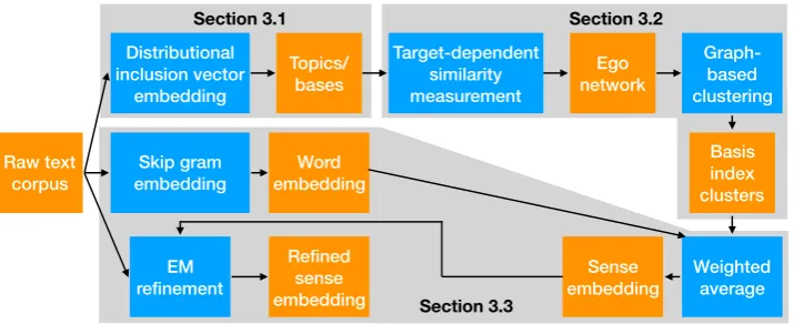
The flowchart of our method is illustrated in Fig-ure 1. We will first briefly introduce distribu-tional inclusion vector embedding (DIVE) (Chang et al.,2018) in Section 3.1, illustrate how we use DIVE as a topic model to construct a graph in Sec-tion3.2, and after clustering the topics, we explain the way to converting each topic cluster to a sense embedding in Section3.3.

3.1 Distributional Inclusion Vector Embedding (DIVE)

Distributional inclusion vector embedding (DIVE) is a variation of skip-gram model (Mikolov et al., 2013). The two major differences compared with skip-gram are that (1) all word embeddings and context embeddings are constrained to be non-negative, and (2) the weights of negative sam-pling for each word is inversely proportional to its frequency. Specifically, the objective function of DIVE is defined by

lDIV E=

X

w

X

c

#(w, c) logσ(wTc) +

kI

X

w

Z

#(w)

X

c

#(w, c) _E cN∼PD

[logσ(₋wTcN)],

(1)

where the word embedding w _≥ 0, the context

embeddingc _≥ 0,cN ≥ 0, #(w, c) are number

of times context wordcco-occur withw,#(w) =

P

c

#(w, c),σ is the logistic sigmoid function,kI

is a constant hyper-parameter, Z is the average #(w)of all words (i.e.,Z =

P w#(w)

|V| and|V|is

the size of vocabulary), andPD is the distribution

of negative samples. The two modifications do not change the time and space complexity of training skip-gram, which is one of the most scalable word embedding methods (Levy et al.,2015).

Raw text corpus

Distributional inclusion vector

embedding

Topics/ bases

Skip gram embedding

Target-dependent similarity measurement

Word embedding

Ego network

Graph-based clustering

Basis index clusters

Weighted average Sense

embedding EM

refinement

Refined sense embedding

Section 3.1 Section 3.2

Section 3.3

Figure 1: The flowchart of the proposed method. The blue boxes are processing steps, the orange boxes are input and output data of each step, and the gray areas indicate the sections describing the included steps.

(SBOW) representation. When the co-occurred context histogram of the word y includes that of

the wordx, it means that for all context wordscin

the vocabularyV,cwill co-occur more times with

y than with x. In this paper, the context words

of a target word means the words co-occur with a target word mention within a small window in the corpus. The default context window size for DIVE is 10. Chang et al.(2018) show that the DIVE is able to compress the sparse bag of words while approximately preserving the inclusion in the low-dimensional space. Formally,

∀c_∈V, #(x, c)_≤#(y, c) ˜

⇐⇒ ∀i_{∈ {}1, ..., L_}, x[i]_≤y[i], (2)

where ⇐⇒˜ means approximately equivalent, #(x, c)and#(y, c) are number of times context word c co-occurs with x and y, respectively. x

andy are the embeddings of the words x andy,

respectively,x[i]is the embedding value of inith

dimension (i.e.,ith basis index). andLis number

of DIVE basis indexes. See Chang et al. (2018) for more the derivation of the equation.

In order to satisfy equation (2), each basis in-dex of DIVE corresponds to a topic and the em-bedding value at that index represents how often the word appears in the topic. This is because if the embedding of one wordyhas higher value in

every dimension (i.e., higher frequency in every topic) than the value of another wordx, the

con-text words c in the topics usually co-occur more

frequently withy than withx. Inversely, ifx

ap-pears more often in one topic thany(i.e., the

em-bedding value ofxin the corresponding dimension

is higher than that ofy), some context wordscin

the topic could co-occur more often with x than

withy.

In Figure2(a), we present three mentions of the word coreand its top 15 basis indexes in DIVE. The word that has a higher value in a basis index is more frequent in the corresponding topic. For example, the top 1-5 words in the second column of the table look more frequent (and usually more general) than the top 101-105 words.

3.2 Graph-Based Clustering

For each target word, we build an ego network whose nodes are the basis indexes relevant to the word. The basis index b is relevant if DIVE of

the target word q has a value wq[b] higher than

a threshold T. The threshold is set to be 1% of average non-zerowq[b]over basis indexes in our

experiment.

Every pair of nodes are linked by an edge weighted by the similarity between the two basis indexes. Each basis indexbi is represented by a

feature vector. A naive way to prepare the feature vector ofith basis indexf(bi)is to use the

embed-ding values in that indexw[bi]of all the words in

our vocabularyV. That is,

f_(bi)= ⊕

w∈Vw[bi], (3)

the operator⊕means concatenation. However, as

… the innovation of the common core , a educational strategy … … both basic cpus and standard product built around a CPU core …

…

…

bj Top 1-5 words Top 101-105 words

1 element, gas, atom, rock, carbon methane, crystalline, complex, surround, proton

2 star, orbit, sun, orbital, planet bright, position, centauri, interaction, universe

3 electron, current, electric, circuit, voltage anode, wire, ac, perform, resistor

4 tank, cylinder, wheel, engine, steel aluminum, automatic, pilot, prevent, remove

5 high, low, temperature, energy, speed atmospheric, fast, blood, m, population

6 acid, carbon, product, use, zinc ph, monoxide, phosphorus, bond, manufacture

7 system, architecture, develop, base, language functional, requirement, processing, compatible, api

8 version, game, release, original, file cassette, virtual, code, project, kb

9 network, user, server, datum, protocol technology, rout, agent, microsoft, command

10 access, need, require, allow, program size, ability, format, run, typically

11 also, well, several, early, see fall, eventually, main, rise, mostly

12 part, almost, see, addition, except incorporate, stage, instead, opening, add

13 several, main, province, include, consist designate, exist, swiss, branch, thai

14 science, philosophy, theory, philosopher, term ethical, advocate, topic, basic, universe

15 school, university, student, education, college doctorate, doctoral, middle, arts, compulsory

… these cold dense

core be the site of future star formation …

wq[bj] of core

Output: embedding of each word (e.g. core)

Input: Plaintext corpus

science

bi

1 2 3 4 5 6 7 8 9 10 11 12 13 14 15

base surface computer main engine

w[bi]*wq[bj]

bj Top 1-5 words

1 element, gas, atom, rock, carbon 2 star, orbit, sun, orbital, planet 3 electron, current, electric, circuit, voltage 4 tank, cylinder, wheel, engine, steel 5 high, low, temperature, energy, speed 6 acid, carbon, product, use, zinc

11 also, well, several, early, see 12 part, almost, see, addition, except 13 several, main, province, include, consist

7 system, architecture, develop, base, language 8 version, game, release, original, file 9 network, user, server, datum, protocol 10 access, need, require, allow, program

14 science, philosophy, theory, philosopher, term 15 school, university, student, education, college

(a)

(b)

(c) _core

surface engine

computer

base

main science

nature

space

province

investigate type

use

1

4 ₈

7

11

13 15

14

(d)

w[bi]*wq[bj] w[bi]*wq[bj] w[bi]*wq[bj] w[bi]*wq[bj] w[bi]*wq[bj]

… f(b3,q)

Figure 2: A visualization of finding the senses of the wordcore.

(a)The DIVEw[bj]of the wordcore(only top 15 basis indexes are shown). The words in each row of the table

are sorted by its embedding value in the basis index.

(b) Weighted DIVE of six words on these 15 basis indexes relevant tocoreas the features for measuring the similarity between basis indexes. The two red boxes indicate two final clusters we discovered at the end within which the feature words tend to have similar embedding values.

(c)The ego network constructed for the wordcore. Each blue box and the corresponding circle represent a basis index or topic (only 8 out of 15 basis indexes are plotted and their index numbersbjare shown in the blue boxes),

which is a node in the network. Two basis indexes are more similar if more relevant words (i.e., close tocore) occur frequently in both corresponding topics. For example, the topic 7 and 8 are more similar because of the frequent appearance of the relevant words such ascomputerin both topics. The larger similarity is represented by a thicker red line. The ego network is a complete graph but only a subset of edges are plotted in the figure. (d)The final clustering results when the number of clusters is set to be 4.

q, we only take the topnwords of every basis

in-dex j in the set Bj(n) instead of considering all

the words in the vocabulary. Then, we weigh the feature based on how likely it is to observe the tar-get word in topic j (wq[bj]) and concatenate all

features together. That is, the feature vector of the

ith dimensionf(bi,q)is defined as:

f_(bi,q)= _⊕L

j=1w∈B⊕j(n)

w[bi]·wq[bj], (4)

wherenis fixed as 100 in the experiment.

irrele-vant bases by defining the similarity between two basis indexes as

SIM(bi, bj, q) = cos(f(bi,q),f(bj,q))·

log(min(wq[bi],wq[bj])

T ),

(5) where cos(f(bi,q),f(bj,q)) is the cosine similarity

between the features of two basis indexes, and the term log(min(wq[bi],wq[bj])

T ) is to prevent

ir-relevant basis indexes in the ego network mis-leading the clustering algorithm. Notice that

SIM(bi, bj, q)≥0because all featuresf(b,q) ≥0

and every node is a relevant basis index b with wq[b]> T.

After the ego network is constructed, we could apply any hierarchical graph clustering. In this pa-per, we just choose spectral clustering with fixed number of clusters for simplicity. In our experi-ment, DIVE with 100 dimensions produces only 6.4 relevant basis indexes on average which needs to be clustered for each target word. This number goes to only 19 for DIVE with 300 dimensions. Thus, we are allowed to use spectral clustering to perform global optimization without inducing large computational overhead in this step.

In Figure 2, we use the target wordcoreas an example to illustrate our clustering algorithm. Af-ter DIVE is trained in (a), we visualize six di-mensions of features for each basis index f_(bi,q)

in (b). Using the features, we can build the ego network as shown in (c). The figure highlights the novelty of our approach. Instead of directly clustering words as other graph-based methods, we group the words first and cluster the groups to form senses. Since the basis is global, we do not have to retrain it given a different target word. DIVE provides us an easy and efficient way to ignore the irrelevant words being far away from corein (c), such asprovinceorspace, and clus-ter based on the words close to the target word such asmainorcomputer. The target-dependent similarity measurement preserves the main spirit of existing graph-based approaches.

3.3 From Basis Index Clusters to Sense Embeddings

As shown in Figure 2 (d), every sense is repre-sented by a group of basis indexes each of which has a weight based on its relevancy to the target word (e.g., the relevancy of bith basis index is wq[bi]). In order to apply existing WSI evaluation

and potentially other downstream applications, we convert the basis index clusters to sense embed-ding.

First, we train a word embedding. Any existing embeddings could be used and we choose skip-gram due to its efficiency. Based on the trained word2vec, we first create a topic embedding for each basis index by averaging skip-gram embed-ding of the top 1000 wordsBi(1000)weighted by

the DIVEw[bi]of the words atbith basis index as

given as:

tbi =

P

w∈Bi(1000)exp(w

0_[bi])·ew

P

w∈Bi(1000)exp(w0[bi])

, (6)

whereewis the skip-gram embedding for the word

whose DIVE arew, and w0 is normalized DIVE such that its average

P

w∈Bi(1000)w0[bi]

1000 = 1. We

take exponential onw0[bi]to focus on the words

that are more important to thebi basis index

be-cause DIVE roughly models thelogof word fre-quency in each topic (Chang et al.,2018).

To generate kth sense embedding sq_k for a

tar-get word q, we take the average of all the topic

embeddings in thekth sense cluster (found in

Sec-tion3.2) weighted by the relevancy between every topic and the target word. Specifically,

sq_k=

P

bi∈Sq_kexp(w0q[bi])·tbi

P

bi∈Sq_kexp(w0q[bi])

, (7)

whereS_kq is the set of basis indexes that belongs

to thekth cluster,w0q is normalized DIVE of the

target word such that its average Pbi∈Nw0q[bi]

|N| =

1, andN is the set of nodes in the ego network.

When converting clusters into embeddings, the previous graph-based WSI methods, such as Pelevina et al.(2016), average the embedding of related words. The average is effective in terms of discriminating the contexts of target word men-tions, but it might not be a good embedding for the sense of target word itself. For instance, one sense embedding ofcorecould be close to the embed-ding ofcomputer, but thecomputer embedding does not represent the sense ofcoreincomputer context as well as the embedding of cpu. Our method suffers the similar problem.

word embedding of the current sentence is clos-est to, and assign the sense to the target token (e.g., bank → bank 1). At M-step, we retrain

the skip-gram using the updated corpus. Our re-finement process could be seen as a simplified ver-sion of multi-sense skip-gram (MSSG) ( Neelakan-tan et al.,2014), which can be easily implemented using existing word embedding library.

4 Experiments

We first conduct a qualitative experiment to ver-ify that our clustering algorithm performs well on some typical polysemy, and show the results in Ta-ble 1. As we can see, our method can not only separate two senses in very different contexts but also can distinguish more subtle sense difference such as identifying thecarcontext and competi-tion context as two different senses of the target wordrace.

Intuitively speaking, our method could be espe-cially useful when it comes to increase the recall of less common senses (like discovering the edu-cational meaning ofcore), but it is hard to verify the claim using existing WSI benchmarks because the common senses, especially the most frequent sense, often dominate in the benchmarks unless using the datasets where the bias is removed. In the following sections, we will first introduce the setup and then the experiments on 3 datasets.

4.1 Experimental Setup

We train DIVE on first 51.2 million tokens of WaCkypedia (Baroni et al.,2009), the dataset sug-gested by Chang et al. (2018), and the default hyper-parameter setting is used except the num-ber of embedding dimensions L (i.e., number of basis indexes). We train two DIVEs, one with 100 dimensions and the other with 300 dimensions to study how the granularity of basis affects the per-formance. For all other steps or baselines, we train them on the whole WaCkypedia where the stop words are removed.

For our clustering module, we use all the default hyper-parameters of the spectral clustering library in Scikit-learn 0.18.2 (Pedregosa et al.,2011) ex-cept the number of clusters is fixed at 2. Setting a number larger than 2 makes it harder to compare with the results generated from other baselines whose default hyper-parameters usually make av-erage number of senses between 1 and 2. Dur-ing EM, we train the skip-gram embeddDur-ing on the

whole WaCkypedia where we treat every consec-utive 20 tokens as a sentence, and the refinement stops after 3 EM iteration. In the tables of this sec-tion, our methods using DIVE with 100 and 300 dimensions are denoted as DIVE (100) and DIVE (300), respectively.

In all quantitative experiments, we compare our method withPelevina et al.(2016), a state-of-the-art graph-based clustering which builds ego graphs based on words similar to the target words, so we call it word graph (WG). To train the model, we first train skip-gram on whole WaCkypedia and use all the default hyper-parameters in their re-leased code to get sense embeddings.2 _{We also} ap-ply our EM refinement step to their output embed-ding to make the comparison fair and call this vari-ation WG+EM. We also compare our method with the baseline which randomly assigns two senses to every token and performs EM to refine the em-bedding (i.e., only adopting our post-processing step). The method is similar to multiple-sense skip-gram (Neelakantan et al., 2014), so we call it MSSG in our tables.

In all datasets, evaluation involves the similarity measurement between a sense of the target word and a context. For each query, we compute co-sine similarity between the context embedding and the sense embedding of the target word, where the context embeddingecis the average embedding of

word in the context. Notice that each word in the context could also be polysemous. In these cases, we adopt the sense embedding of the context word that is closest to the sense of the target word (i.e., highest cosine similarity).

4.2 Word Context Relevance (WCR)

Given a target word, the task (Arora et al.,2016; Sun et al.,2017) is to identify the true context cor-responding to a sense of the target word out of 10 other randomly selected false contexts, where a context is presented by similar words. For ex-ample, two of the true contexts for the target word bank are water,land,river,... and institu-tion,deposits,money.... We use the R1 dataset fromSun et al.(2017), which consists of 137 word types and 535 queries.

For each query pair (target wordwq, contextc),

we compute the similarity between each sense of target wordsq_kand the contextec, and choose the

Query CID Top 5 words in the top dimensions

rock 1

element, gas, atom, rock, carbon sea, lake, river, area, water find, specie, species, animal, bird point, side, line, front, circle 2 _{early, work, century, late, begin}band, song, album, music, rock _{include, several, show, television, film}write, john, guitar, band, author

bank 1

county, area, city, town, west several, main, province, include, consist building, build, house, palace, site sea, lake, river, area, water

2 _{united, states, country, world, europe}money, tax, price, pay, income company, corporation, system, agency, service_{state, palestinian, israel, right, palestine}

apple

1 food, fruit, vegetable, meat, potato goddess, zeus, god, hero, sauron war, german, ii, germany, world write, john, guitar, band, author 2 _{system, architecture, develop, base, language}version, game, release, original, file car, company, sell, manufacturer, model_{include, several, show, television, film}

star 1

film, role, production, play, stage character, series, game, novel, fantasy wear, blue, color, instrument, red write, john, guitar, band, author 2 element, gas, atom, rock, carbon star, orbit, sun, orbital, planet

give, term, vector, mass, momentum light, image, lens, telescope, camera

tank

1 tank, cylinder, wheel, engine, steel_{acid, carbon, product, use, zinc} industry, export, industrial, economy, company_{network, user, server, datum, protocol} 2 _{however, attempt, result, despite, fail}army, force, infantry, military, battle aircraft, navy, missile, ship, flight_{war, german, ii, germany, world}

race

1 win, world, cup, play, championship two, one, three, four, another 2 railway, line, train, road, rail car, company, sell, manufacturer, model 3 population, language, ethnic, native, people female, age, woman, male, household

run 12 system, architecture, develop, base, languagerailway, line, train, road, rail access, need, require, allow, programalso, well, several, early, see 3 game, team, season, win, league game, player, run, deal, baseball

tablet 12 use, system, design, term, methodbc, source, greek, ancient, date version, game, release, original, filebook, publish, write, work, edition 3 system, blood, vessel, artery, intestine patient, symptom, treatment, disorder, may

Table 1: Examples of sense clusters on polysemous words. When the number of clusters is set to be 2, we present the top 4 basis indexesbjin each sense cluster, which have the highest values on the target word embeddingwq[bj].

Otherwise, the top 2 basis indexes are presented. CID refers to sense cluster ID. The top 5 words with the highest values of each basis indexw[bj]are presented.

senses of the target word with maximal similarity (i.e., SIM(wq,ec) = maxkcos(sqk,ec)). Then,

we rank the similarity of 11 query pairs, which consist of 1 true context and 10 false contexts. The performance of different methods is evaluated by checking whether the top 1 (i.e., the pair with the highest similarity) is true. The metric (Sun et al., 2017) is called Precision@1.

The results are shown in Table 2. Since the task is to identify the related contexts, skip-gram is a good baseline (Sun et al., 2017). In this dataset, each sense is equally important, regard-less how often the sense appears in the corpus. The significantly better performance from DIVE demonstrates our capability of modeling more fine-grained senses of polysemous words.

4.3 TWSI Evaluation

The Turk bootstrap Word Sense Inventory (TWSI) task (Biemann,2012) is based on a large dataset,

Skip-gram WG WG+EM

52.7 42.1 59.1

MSSG DIVE (100) DIVE (300)

60 63.2 62.6

Table 2: Precision@1 on the WCR R1 (%).

which consists of 1,012 nouns accompanied with 145,140 context sentences. The task is to identify the correct sense of the target nouns, and all WSI algorithms choose the sense whose embedding is most similar to the context embedding.

Model _P TWSI_{R F1 P}balanced TWSI_{R F1} MSSG rnd 66.1 65.7 65.9 33.9 33.7 33.8

MSSG 66.2 65.8 66.0 34.3 34.2 34.2 WG 68.6 68.1 68.4 38.7 38.5 38.6 WG+EM 68.3 67.8 68.0 38.4 38.2 38.3 DIVE rnd 63.4 63.0 63.2 33.4 33.2 33.3 DIVE (100) 67.6 67.2 67.4 39.7 39.5 39.6 DIVE (300) 67.4 66.9 67.2 39.0 38.8 38.9

Table 3: Results obtained on the TWSI task (%), where P is precision and R is recall. MSSG rnd and DIVE rnd are baselines which randomly assign sense given inventory built by MSSG and DIVE, respectively.

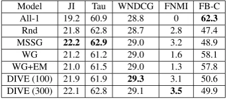
Model JI Tau WNDCG FNMI FB-C

All-1 19.2 60.9 28.8 0 62.3

Rnd 21.8 62.8 28.7 2.8 47.4

MSSG 22.2 62.9 29.0 3.2 48.9

WG 21.2 61.2 29.0 1.6 58.1

WG+EM 21.0 61.5 29.0 1.3 57.8

DIVE (100) 21.9 61.9 29.3 3.1 50.6 DIVE (300) 22.1 62.8 29.1 3.5 49.9

Table 4: Results obtained on the SemEval 2013 task (%), where JI is Jaccard Index, FNMI is Fuzzy NMI, and FB-C is Fuzzy B-Cubed. All-1 is to assign all senses to be the same and Rnd is to randomly assign all senses to 2 groups.

When evaluating on TWSI, each method needs to represent the sense by a sparse bag-of-word context feature called sense inventory. The eval-uation script3 _{first maps each sense predicted by} each algorithm to a ground truth sense. Then, the problem becomes a classification task, which can be evaluated by precision, recall, and F1.

In Table 3, we can see that DIVE performs slightly worse than WG (Pelevina et al., 2016) in full TWSI, but becomes slightly better in balanced TWSI. We suspect this is because our number of sense is 2 but the WG generates the output where the average number of senses is around 1.5, which might do better when a sense of each word oc-curs most of the time. Notice that the compari-son in balanced TWSI is fair because the experi-ments inPelevina et al.(2016) show that WG per-forms worse when increasing number of clusters. The results also suggest that a sufficient number of basis vectors seldom group two senses together (otherwise, increasing the resolution/dimension of DIVE should be helpful).

3_{https://github.com/tudarmstadt-lt/} context-eval

4.4 SemEval-2013 task 13 Evaluation

SemEval-2013 task 13 (Jurgens and Klapaftis, 2013) provides a smaller dataset which consists of 50 words which include nouns, verbs, and adjec-tives. The context prediction is done in the same way as TWSI, and the meaning of each metric could be found inJurgens and Klapaftis(2013). In Table4, we can see our method performs roughly the same compared with other baselines.

5 Conclusions

We propose a novel graph-based WSI approach. In order to save the time of performing a near-est neighbor search, we first group words into ba-sis/topics using distributional inclusion vector em-bedding (DIVE), compute target-dependent sim-ilarity between basis indexes, and then perform graph clustering. Our experimental results show that the method achieves the state-of-the-art per-formances and is able to capture less common senses with higher accuracy.

6 Acknowledgement

This material is based upon work supported in part by the Center for Data Science and the Cen-ter for Intelligent Information Retrieval, in part by Lexalytics, in part by the Chan Zuckerberg Initiative under the project Scientific Knowledge Base Construction, and in part by the National Sci-ence Foundation under Grant No. IIS-1514053 and No. DMR-1534431, in part using high per-formance computing equipment obtained under a grant from the Collaborative R&D Fund managed by the Massachusetts Technology Collaborative. Any opinions, findings and conclusions or recom-mendations expressed in this material are those of the authors and do not necessarily reflect those of the sponsor.

References

Eneko Agirre, David Mart´ınez, Oier Lopez de Lacalle, and Aitor Soroa. 2006. Two graph-based algorithms for state-of-the-art WSD. In EMNLP 2007, Pro-ceedings of the 2006 Conference on Empirical Meth-ods in Natural Language Processing, 22-23 July 2006, Sydney, Australia.

Sanjeev Arora, Yuanzhi Li, Yingyu Liang, Tengyu Ma, and Andrej Risteski. 2016. Linear algebraic struc-ture of word senses, with applications to polysemy.

Ben Athiwaratkun and Andrew Gordon Wilson. 2017. Multimodal word distributions. InACL.

Marco Baroni, Silvia Bernardini, Adriano Ferraresi, and Eros Zanchetta. 2009. The WaCky wide web: a collection of very large linguistically processed web-crawled corpora. Language resources and

evaluation43(3):209–226.

Sergey Bartunov, Dmitry Kondrashkin, Anton Osokin, and Dmitry P. Vetrov. 2016. Breaking sticks and am-biguities with adaptive skip-gram. InProceedings of the 19th International Conference on Artificial Intel-ligence and Statistics, AISTATS 2016, Cadiz, Spain,

May 9-11, 2016.

Chris Biemann. 2006. Chinese whispers: an efficient graph clustering algorithm and its application to nat-ural language processing problems. InProceedings of the first workshop on graph based methods for natural language processing.

Chris Biemann. 2012. Turk bootstrap word sense in-ventory 2.0: A large-scale resource for lexical sub-stitution. InProceedings of the Eighth International Conference on Language Resources and Evaluation,

LREC 2012, Istanbul, Turkey, May 23-25, 2012.

Haw-Shiuan Chang, ZiYun Wang, Luke Vilnis, and Andrew McCallum. 2018. Distributional inclusion vector embedding for unsupervised hypernymy de-tection. In Human Language Technology Confer-ence of the North American Chapter of the

Associa-tion of ComputaAssocia-tional Linguistics (HLT/NAACL).

Antonio Di Marco and Roberto Navigli. 2013. Cluster-ing and diversifyCluster-ing web search results with graph-based word sense induction. Computational

Lin-guistics39(3):709–754.

Beate Dorow and Dominic Widdows. 2003. Discov-ering corpus-specific word senses. In EACL 2003, 10th Conference of the European Chapter of the As-sociation for Computational Linguistics, April

12-17, 2003, Agro Hotel, Budapest, Hungary.

David Hope and Bill Keller. 2013. Maxmax: a graph-based soft clustering algorithm applied to word sense induction. In International Conference on Intelligent Text Processing and Computational Lin-guistics.

David Jurgens and Ioannis Klapaftis. 2013. Semeval-2013 task 13: Word sense induction for graded and non-graded senses. InSecond Joint Conference on Lexical and Computational Semantics (* SEM), Vol-ume 2: Proceedings of the Seventh International

Workshop on Semantic Evaluation (SemEval 2013).

Jey Han Lau, Paul Cook, Diana McCarthy, David New-man, and Timothy Baldwin. 2012. Word sense in-duction for novel sense detection. InEACL 2012, 13th Conference of the European Chapter of the As-sociation for Computational Linguistics, Avignon, France, April 23-27, 2012.

Omer Levy, Yoav Goldberg, and Ido Dagan. 2015. Im-proving distributional similarity with lessons learned from word embeddings. Transactions of the

Associ-ation for ComputAssoci-ational Linguistics3:211–225.

Jiwei Li and Dan Jurafsky. 2015. Do multi-sense em-beddings improve natural language understanding?

InProceedings of the 2015 Conference on Empirical

Methods in Natural Language Processing, EMNLP

2015, Lisbon, Portugal, September 17-21, 2015.

Dekang Lin et al. 1998. An information-theoretic defi-nition of similarity. InICML.

Binny Mathew, Suman Kalyan Maity, Pratip Sarkar, Animesh Mukherjee, and Pawan Goyal. 2017. Adapting predominant and novel sense discovery al-gorithms for identifying corpus-specific sense differ-ences. InProceedings of TextGraphs@ACL 2017: the 11th Workshop on Graph-based Methods for Natural Language Processing, Vancouver, Canada, August 3, 2017.

Tomas Mikolov, Ilya Sutskever, Kai Chen, Greg S Cor-rado, and Jeff Dean. 2013. Distributed representa-tions of words and phrases and their compositional-ity. InNIPS.

George A. Miller. 1995. Wordnet: a lexical database for english. Communications of the ACM

38(11):39–41.

Sunny Mitra, Ritwik Mitra, Martin Riedl, Chris Bie-mann, Animesh Mukherjee, and Pawan Goyal. 2014. That’s sick dude!: Automatic identification of word sense change across different timescales. In

Proceedings of the 52nd Annual Meeting of the As-sociation for Computational Linguistics, ACL 2014, June 22-27, 2014, Baltimore, MD, USA, Volume 1: Long Papers.

Jiaqi Mu, Suma Bhat, and Pramod Viswanath. 2017. Geometry of polysemy. InICLR.

Roberto Navigli and Giuseppe Crisafulli. 2010. Induc-ing word senses to improve web search result clus-tering. In Proceedings of the 2010 conference on

empirical methods in natural language processing.

Arvind Neelakantan, Jeevan Shankar, Alexandre Pas-sos, and Andrew McCallum. 2014. Efficient non-parametric estimation of multiple embeddings per word in vector space. InProceedings of the 2014 Conference on Empirical Methods in Natural Lan-guage Processing, EMNLP 2014, October 25-29, 2014, Doha, Qatar, A meeting of SIGDAT, a Special Interest Group of the ACL.

Patrick Pantel and Dekang Lin. 2002. Discovering word senses from text. InProceedings of the eighth ACM SIGKDD international conference on Knowl-edge discovery and data mining.

E. Duchesnay. 2011. Scikit-learn: Machine learning in Python. Journal of Machine Learning Research

12(Oct):2825–2830.

Maria Pelevina, Nikolay Arefiev, Chris Biemann, and Alexander Panchenko. 2016. Making sense of word embeddings. InProceedings of the 1st Workshop on Representation Learning for NLP, Rep4NLP@ACL

2016, Berlin, Germany, August 11, 2016.

Luis Nieto Pi˜na and Richard Johansson. 2015. A sim-ple and efficient method to generate word sense rep-resentations. In Recent Advances in Natural Lan-guage Processing, RANLP 2015, 7-9 September, 2015, Hissar, Bulgaria.

Joseph Reisinger and Raymond J. Mooney. 2010. Multi-prototype vector-space models of word mean-ing. InHuman Language Technologies: Conference of the North American Chapter of the Association of Computational Linguistics, Proceedings, June 2-4, 2010, Los Angeles, California, USA.

Hinrich Sch¨utze. 1992. Dimensions of meaning. In

Proceedings of the 1992 ACM/IEEE conference on

Supercomputing.

X Yu Stella and Jianbo Shi. 2003. Multiclass spectral clustering. InICCV.

Chiraag Sumanth and Diana Inkpen. 2015. How much does word sense disambiguation help in sentiment analysis of micropost data? InProceedings of the 6th Workshop on Computational Approaches to Sub-jectivity, Sentiment and Social Media Analysis.

Yifan Sun, Nikhil Rao, and Weicong Ding. 2017. A simple approach to learn polysemous word embed-dings. arXiv preprint arXiv:1707.01793.

Fei Tian, Hanjun Dai, Jiang Bian, Bin Gao, Rui Zhang, Enhong Chen, and Tie-Yan Liu. 2014. A probabilis-tic model for learning multi-prototype word embed-dings. InCOLING.

Jean V´eronis. 2004. Hyperlex: lexical cartography for information retrieval. Computer Speech &