To preliminary test or not to preliminary
test, that is the question.
Applied Statistics Group
Research
Students
Conference in
Probability and
Statistics, 2018
How to compare two
independent samples?
Calculate the skewness
Always use the independent samples t-test
Always use the Mann-Whitney test
Graphical assessment of assumptions
Always use Welch’s test
Look at sample size
Perform formal hypothesis tests of assumptions
Use the test that best supports my conclusions
Check for outliers
Example
Group 1
9
12
12
12
12
12
13
13
13
14
14
14
Group 2
9
10
11
14
15
15
15
16
16
17
18
19
Preliminary test for equal variances
Levene’s test
Brown-Forsythe test
p = .030
Reject null hypothesis of equal variances.
p = .071
Fail to reject null hypothesis of equal variances.
Two-sample test conditional upon result of preliminary test
Welch’s test
Independent samples t-test
p = .051
Fail to reject the null hypothesis that the two
samples means do not differ.
p = .046
Reject the null hypothesis that the two samples
means do not differ.
Simulation study
Preliminary tests for normality:
• Shapiro-Wilk test (SW)
• Kolmogorov-Smirnov test (KS).
Preliminary tests for equality of variances:
• Levene's test (L)
Simulation study
Preliminary tests, 0%-10% significance level [1% increments]
Conditional tests at 5% significance level, selected based on
results of each of the preliminary test combinations.
Sample sizes varied within a factorial design: 5, 10, 20, 30.
10,000 iterations.
Distributions:
• Standard Normal
• Normal unequal variances
• Exponential
Discussion
• All procedures liberal under normality with unequal variances.
• All procedures perform similarly.
Conclusion
Preliminary testing valid
However;
• May not be necessary
• If performed, pre-defined plan is required
Supporting material
Derrick, B. (2018). To preliminary test or not to
preliminary test, that is the question. In: Research
Students Conference in Probability and Statistics.
Available from: http://eprints.uwe.ac.uk
‘There is nothing either good or bad, but thinking makes it so'
William Shakespeare, Hamlet Act 2 Scene 2
‘It is our choices...that show what we truly are, far more than our abilities'
Research Students Conference in Probability and Statistics, 2018
To preliminary test or not to preliminary test, that is the question.
Despite the consequences of violations to the assumptions of statistical tests, there is often neglect in published works to report on the assumptions of the tests performed. Preliminary testing the assumptions prior to preforming the test is done routinely by some researchers, and some do in an ad-hoc manner. Literature and opinions on these contrasting approaches are discussed. Complications with preliminary testing arise due to each assumption having many possible preliminary tests that could be performed. In addition the arbitrary 5% significance level is often used but this need not be standard. In the comparison of two independent samples, the significance level for the preliminary tests is considered, along with two preliminary tests for equality of variances, and two preliminary tests for normality. The results indicate that preliminary testing may not be unreasonable, if the analysis strategy is determined at the study design stage.
‘There is nothing either good or bad, but thinking makes it so’ William Shakespeare, Hamlet Act 2 Scene 2
‘It is our choices...that show what we truly are, far more than our abilities’ JK Rowling, Harry Potter and the Chamber of Secrets
Introduction
Despite the consequences of violations to the assumptions of frequently per-formed statistical tests, there is often neglect in published work to report on the assumptions of the tests being performed. The American Psychological Association for example does not instruct researchers to check for violations of assumptions, or to report the checks performed (APA, 2018). Ignoring vio-lations of assumptions when test statistics are not robust breaches Statistical Conclusion Validity (SCV), the extent to which data from a research study can be regarded as revealing a link as far as statistical issues are concerned (Cook, Campbell, and Day, 1979).
Some researchers choose to do one or more preliminary tests of the as-sumptions before proceeding with the test on the null hypothesis of interest. When a preliminary test informs the user which test on the hypothesis of interest to perform, the resulting test is referred to as a conditional test.
As an illustration, in the case of choosing a one sample test for central location, Weir, Gwynllyw, and Henderson (2017) advocate performing formal hypothesis tests for normality for small to moderate sample sizes (preliminary tests), the result determines whether the one sample t-test or the one sample Wilcoxon signed rank test is performed (conditional tests).
Advocates of a preliminary testing approach for the comparison of two independent samples include Gurland and McCullough (1962) and Gebski and Keech (2003). A well defined preliminary testing strategy can ensure an appropriate test for central location is performed (Wells and Hintze, 2007).
Ideally assumptions should be assessed based on prior knowledge, study design, or preliminary testing of test data (Wells and Hintze, 2007).
Authors against preliminary testing include Zimmerman (2004) and Ro-chon, Gondan, and Kieser (2012). When performing a preliminary test of an assumption, a valid test will reject the assumption as dictated by the signifi-cance level of the preliminary test. The conditional test will also have a Type I error rate. This double testing increases the chances of Type I errors and thus can be detrimental to SCV (Moser and Stevens, 1992; Rasch, Kubinger, and Moder, 2011).
García-Pérez (2012) suggest that to achieve SCV researches should select tests that match the study design, and that Type I error rates match those declared in the limitations of the validity of conclusions.
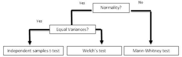
Figure 1 shows a frequently performed two sample test procedure for two independent samples (Weir, 2018).
Figure 1: A typical two independent samples test procedure
There are numerous ways in which the assumptions in Figure 1 could be checked.
Some may use graphical representation instead of formal preliminary test-ing, but this does not eliminate the problem, because the decision on the analysis is nevertheless conditional on the results of preliminary analysis (García-Pérez, 2012). Furthermore, graphical assessment gives rise to sub-jective interpretation, human error and human bias.
[image:12.595.167.469.476.571.2]Some two sample test procedures may incorporate skewness and kurtosis for informing the appropriate conditional test. For a comparison of two inde-pendent samples Kim (2013) suggest that if the skewness or kurtosis exceeds 1.96 then assume non-normality, although no supporting references for this approach are offered. Fagerland (2012) does not agree with the premise of assessing skewness and suggest that for large sample sizes the parametric test should always be applied. Other ad hoc methods for determining which two sample test to perform are available throughout the Internet e.g. Anderson (2014) or Mayfield (2013), they rarely have supporting references, and have the common theme of being relatively vague how to assess the assumptions. Hoekstra, Kiers, and Johnson (2012) investigated the approach by psy-chology PhD students in the Netherlands when faced with a research question comparing two independent samples, among other scenarios. In total 30 stu-dents completed the experiment, approximately 1 in 4 checked the assump-tion of normality (in these cases no formal preliminary test was performed), and approximately 1 in 3 checked the assumption of equal variances (in these cases a formal preliminary test was common). Of those that did not check the assumptions, in a follow up survey, the majority suggested that they were unfamiliar with the assumptions. Approximately 2 in 3 were unfamiliar how to check the assumption, and less than 1 in 3 said they regarded the test as robust to violations of the assumption and therefore did not need to check.
Publication bias, where only statistically significant findings are pub-lished, leads to a temptation by some researchers to adopt practices such as data dredging or fishing. Publication bias also leads to a temptation by some researchers to report the findings of the test that show the most significant effect. Inconsistent advice regarding preliminary testing offers researchers opportunity to exploit this practice. Performing preliminary testing based on a pre-defined set of rules can lead to inertia and apathy with regards to the conditional test used. Conversely, some researchers may perform pre-liminary testing on an ad-hoc basis, and reverse engineer the prepre-liminary testing procedure to achieve desired conclusions. This has contributed to the reproducibility crisis in the sciences.
A further preliminary testing consideration is the optimum significance level to work at for the preliminary tests. The arbitrary 5% significance level is usually used but this need not be standard.
In the following, preliminary test for normality are considered followed by preliminary tests for equal variances. Using two of the most commonly performed tests for normality and equal variances a simulation study is de-vised to explore the Type I error robustness of different combinations of these preliminary tests at different significance levels.
Preliminary tests for normality
In real life, normality does not exist (Micceri, 1989), however the applica-tion of some models is useful (Box, 1976). Normality is desirable because parametric tests such as the t-test are more powerful than alternative non-parametric tests under this condition (Fagerland, 2012).
Given the independent samples t-test assumption that two samples arise from the same normally distributed population, and the debated robustness of statistical tests, standard practice is to first test the samples for normality (Mahdizadeh, 2018). It should be noted that it is more appropriate to test normality of residuals rather than the data itself (Totton and White, 2011). There are numerous tests for normality (Razali, Wah, et al., 2011). Ex-ample tests for normality are the Shapiro-Wilk test and the Epps-Pulley test. These two tests are the recommended tests and in a practical sense there is little to choose between them (ISO 5479 1997). The Sharipo-Wilk test was originally intended for sample sizes up to 50 (Razali, Wah, et al., 2011). Mendes and Pala (2003) who used simulation for samples sizes up to 200 demonstrated that the Shapiro-Wilk test is Type I error robust regardless of sample size. For small sample sizes, the Shapiro-Wilk test lacks power to de-tect deviations from normality (Rochon, Gondan, and Kieser, 2012; Razali, Wah, et al., 2011).
The most commonly applied normality test is the Kolmogorov-Smirnov test (Ghasemi and Zahediasl, 2012). This is likely because it is readily avail-able in most statistical software and can be used to test a data set against any distribution. When testing for normality, the Kolmogorov-Smirnov test is more liberal, and therefore less sensitive than the Shapiro-Wilk test (Shapiro, Wilk, and Chen, 1968). The Shapiro-Wilk test has good power and has there-fore become the most widely advocated test for normality (Razali, Wah, et al., 2011; Mendes and Pala, 2003; Ghasemi and Zahediasl, 2012). Tests for normality are widely researched, with authors striving for and continuing to develop more powerful tests for normality (Mahdizadeh, 2018). How-ever, for preliminary testing of assumptions, the insensitive nature of the Komologorov-Smirnov test to minor deviations from normality could be ad-vantageous in a practical environment, due to the robustness of parametric tests.
Lumley et al. (2002) suggest that for large samples in public health data there is no requirement for a normalilty assumption. With smaller sample sizes, Lumley et al. (2002) conclude that tests for non-normality is undesir-able as they have low power and they detract from the real assumptions of these methods.
Using 10,000 iterations of equally sized samples Rochon, Gondan, and
Kieser (2012) investigated the Type I error of conditional tests, performing the Sharipo-Wilk test for normality followed by the independent samples t-test or the Mann-Whitney test as determined from the result of the nor-mality test. Rochon, Gondan, and Kieser (2012) inform that performing the Sharipo-Wilk test first maintains the nominal significance level for normally and uniformly distributed data. However, for exponentially distributed pop-ulations, the preliminary testing process increases the probability of making Type I error. Therefore tests for normality may be reasonable if the data are symmetric. The authors conclude that the preliminary testing does little harm and is more a waste of time, the authors re-iterate that the t-test is robust in many situations. Given their assertion that normality is a myth, Micceri (1989) also dismiss this preliminary testing process as futile.
Preliminary tests for equal variances
For unequal sample sizes, statisticians are still debating the conditions for which the independent samples t-test is robust, when the assumption of equal variances is violated (Nguyen et al., 2012). As a result of this uncertainty, common practice is to first test for equality of variances prior to performing a test of means.
It should be noted that testing the difference in sample variances does not necessarily equate to testing the differences in the population variances. Especially for small sample sizes, you would expect to see some deviation in sample variances from true variances.
Zimmerman and Zumbo (2009) consider the impact of performing both the independent samples t-test and Welch’s test, they raise the concern that publication bias tempts users to perform both and then plump for the that shows the desired significant result. They show that for populations with equal variances, at least one of the two tests would indicate unequal vari-ances a higher proportion of the time than the nominal significance level. Conversely with unequal variances, these would appear equal a higher pro-portion of the time than expected from each test individually. Both are true even with relatively medium sample sizes (20-40). As the group variances tend towards equality, the probability of rejecting the null hypothesis using conditional testing is biased more than from using a single test.
In SAS the proc ttest procedure provides analyses using the independent sample t-test unconditionally, Welch’s test unconditionally (referred to as Satterthwaite’s test in SAS), and one of these two tests selected conditional upon result of an F-test assessing for homogeneous variances. This approach was investigated by Nguyen et al. (2012) for normally distributed data. They
found that when sample sizes are equal, the independent samples t-test is the most Type I error robust. In addition, when sample sizes are unequal, Welch’s test and the conditional test procedure perform the best against Bradley’s (1978) liberal robustness criteria. They also found that, as the sample size ratio increases, Welch’s tests maintains the nominal Type I error rate slightly better than the conditional test procedure (likely due to the double testing applied under conditional testing). Larger sample sizes do not improve the Type I error rate for the independent samples t-test, but do for the conditional procedure and Welch’s test. The conditional test procedure showed a very slight power advantage, however power cannot be reasonably compared if the Type I error rates are not the same (Penfield, 1994). When including samples with skewness and kurtosis to the above simulation, Kellermann et al. (2013) reasonably replicate the conclusions by Nguyen et al. (2012) for all nominal significance levels. Under non-normality their results suggests that the independent samples t-test is generally robust. In these scenarios the sample size required is greater for the conditional method and Welch’s test to stay within Bradley’s liberal criteria.
For unequal sample sizes, Nguyen et al. (2012) and Kellermann et al. (2013) questioned the use of the 5% significance level for preliminary tests. They say that if the F-test reports a significant difference in the variances using a specifiedαvalue, Welch’s test should be used, otherwise the indepen-dent samples t-test should be used. This criticalαvalue was 0.20 for normal distributions considered by Nguyen et al. (2012) and 0.25 for the distribu-tions considered by Kellermann et al. (2013). Therefore only weak evidence of unequal variances is required before Welch’s test becomes the preferred test. Given these findings and the opinion that nothing is lost from using Welch’s test (Ruxton, 2006), the standard historical approach of testing for equal variances and at some cut off point when variances are significantly different using Welch’s test, otherwise defaulting to Student’s test, seems to be an illogical approach. Instead the approach could potentially be revised to make Welch’s test the default test, and at some cut off point where variances are similar use the independent samples t-test.
A widely used test for equality of variances is Levene’s test, which in the two group case is equivalent to the independent samples t-test on absolute deviations from the mean. A modified Levene’s test using absolute deviations from the median, known as the Brown-Forsythe method is computationally more complex, but is more widely recognised for its robustness (Nordstokke and Zumbo, 2007; Zimmerman, 2004).
Zimmerman (2004) found that when performing Levene’s test as a prelim-inary test, the overall Type I error rate was less than the nominal significance level when the higher sample size was associated with the higher variance,
but more than the nominal when the reverse was true.
Generally it is not a good idea to test for homogeneity of variances, and this approach in its present form is no longer widely recommended (Zimmer-man, 2004). The decision to either use the independent samples t-test or Welch’s test should be made at the design stage of an experiment (Zumbo and Coulombe, 1997).
That said, the independent samples t-test is clearly inadequate for in-creasingly unequal variances (Zimmerman and Zumbo, 2009; Kellermann et al., 2013), and Welch’s test should be used in these situations instead (Der-rick, Toher, and White, 2016). Zimmerman and Zumbo (2009) and Zim-merman (2004) both recommend performing Welch’s test whenever sample sizes are unequal. In fact, their simulation results show that the Welch’s test performs well with respect to Type I errors in every scenario they considered. Based on results similar to this, Ruxton (2006) suggested the routine use of Welch’s test. This approach results in a loss of power when the variances are equal, but a power gain when they are not. However, Fairfield-Smith (1936) re-iterate that there is no uniformly most powerful and unbiased test.
Another issue if performing a preliminary test for equal variances is that different tests for equality of variances give different results, thus informing to use different tests for the comparison of means. For example SPSS and Minitab both report values for ‘Levene’s test’ but the results are not the same. SPSS uses the classical Levene’s test based on the absolute deviations from the mean, whereas Minitab uses the modified Brown-Forsythe test based on the absolute deviations from the median. In fact there are dozens of proposed tests for equal variances. For a comparison of variances, in their flowchart Anderson (2014) remain ambiguous as to which test to perform, and cite three such tests without stating which to perform when and without supporting reference.
In a comparison of fifty-six tests using simulation, Conover, Johnson, and Johnson (1981) narrow it down to three tests which are the most robust, one of which is the Brown-Forsythe test using absolute deviations from the median. Nevertheless a judgement is required, so it could be argued that a practitioner might just as well simply make a judgement on which form of the t-test to use using prior knowledge. For a completely randomised design it is fair to assume equal variances given that both groups are being filled at ran-dom from the same population. For naturally occurring groups, for example if groups are split between male and female, a judgment is needed whether equal variances can be assumed, but it is likely that it is not reasonable in this instance (Zumbo and Coulombe, 1997).
Simulation Study
In the following simulation investigation, the significance level for the pre-liminary tests is considered for two competing tests for assessing equality of variances, and two competing tests for assessing normality.
The impact of altering the significance level for the preliminary tests is considered via simulation, while performing the conditional test of interest each time at the 5% significance level. In a two independent samples design, each of the Mann-Whitney test, the independent samples t-test and Welch’s test are performed to compare two generated samples.
The preliminary tests for normality performed are the Shapiro-Wilk test (SW) and the Kolmogorov-Smirnov test (KS). The tests for equality of vari-ances are Levene’s test (L) and the Brown-Forsythe test (BF). Each prelim-inary test is performed on each conditional test.
The preliminary tests are performed at the 0% to the 10% significance level in increments of 1%. The conditional test is calculated based on the results of each of the preliminary test combinations.
The sample sizes varied within a factorial design are 5, 10, 20 and 30. For each sample size, preliminary test and significance level combination the process is repeated for 10,000 iterations. The proportion of the 10,000 iterations where the null hypothesis is rejected is the Type I error rate of the conditional test. The Type I error rate of the overall test procedure is calculated as the weighted average Type I error rate across each of the conditional tests.
The first set of simulations is performed where both samples are taken from a N(0,1). The process is repeated where one sample is taken form N(0,1) and the other is taken from N(0,4). The process is further repeated where both samples are taken form the Exponential distribution and then when both samples are taken from the Lognormal distribution.
Results
An overview of the results of the simulation study are given in Table 1. Even for the most skewed distribution considered, Table 1 indicates that the procedure identified in Figure 1 is Type I error robust because none of the Type I error rates greatly deviate from 5%.
When samples are drawn from the normal distribution with equal vari-ances, each of the decision rules applied for selecting the conditional test are all approximately equally Type I error robust. This is because all of the tests are Type I error robust under normality and equal variances, therefore
Table 1: Robustness of preliminary testing procedure in Figure 1
Preliminary tests Normal σ12 =σ12 Normal σ21 6=σ12 Exponential Lognormal SW 1%, L 1% 0.050 0.058 0.042 0.038 SW 5%, L 5% 0.051 0.057 0.052 0.046 SW 10%, L 10% 0.052 0.057 0.058 0.049 SW 1%, L 10% 0.053 0.058 0.056 0.050 SW 10%, L 1% 0.049 0.058 0.047 0.043 KS 1%, L 1% 0.051 0.060 0.050 0.046 KS 5%, L 5% 0.053 0.061 0.050 0.046 KS 10%, L 10% 0.054 0.061 0.049 0.046 KS 1%, L 10% 0.054 0.059 0.053 0.047 KS 10%, L 1% 0.051 0.061 0.049 0.046 KS 1%, L 1% 0.051 0.062 0.051 0.048 KS 5%, L 5% 0.053 0.063 0.050 0.047 KS 10%, L 10% 0.055 0.063 0.050 0.046 KS 1%, L 10% 0.054 0.062 0.053 0.047 KS 10%, L 1% 0.051 0.063 0.050 0.047 KS 1%, BF 1% 0.050 0.060 0.044 0.045 KS 5%, BF 5% 0.051 0.060 0.047 0.043 KS 10%, BF 10% 0.052 0.059 0.053 0.045 KS 1%, BF 10% 0.054 0.060 0.048 0.041 KS 10%, BF 1% 0.049 0.060 0.049 0.047
the preliminary testing performed is irrelevant. When the two samples come from normal distributions with unequal variances, the Type I error rate is inflated by performing preliminary tests, however this inflation is within a liberal tolerable region as defined by Bradley (1978).
Across all of the distributions, the procedure that is the ’best’ with the lowest average absolute deviation from the nominal significance level is to perform the Shapiro-Wilk test at the 5% significance level and Levene’s test at the 5 significance level.
The robustness of the overall test procedure is not greatly impacted by altering the significance level of the preliminary test within the simulated range. Furthermore the robustness of the test procedure is not greatly im-pacted by the combination of preliminary tests. Thus the large range of dif-ferent strategies for preliminary testing being used are not necessarily poor strategies, but the question becomes a more philosophical debate about the potential for manipulation and the selection of a strategy for the wrong rea-sons.
Discussion
Performing any of the above preliminary testing strategies appears to do little harm. However, the overall Type I error robustness of the procedure masks the fact that a non robust test may be performed on some occasions, even though the overall procedure is robust. For instance, when the two samples are from the normal distribution with unequal variances, the procedure will more often than not guide the researcher to perform Welch’s test, although the independent samples t-test may not be robust in itself, but because so few simulated instances will return the independent samples t-test, the overall procedure is deemed to be robust.
Using the same simulation methodology but for a slightly different deci-sion tree which incorporates the Yuen-Welch test when variances are unequal and normality assumption is false, Pearce and Derrick (2018) recommended the two-stage preliminary testing procedure with a Kolmogorov-Smirnov nor-mality test and Levene’s test for equal variances, both at the 5% significance level. This is identified for the purposes of adopting a consistent approach only, one which closely maintains Type I error robustness across the dis-tributions simulated. As with the current strategy in Figure 1, Pearce and Derrick (2018) noted that for this alternative strategy there really is not much to choose between the different preliminary tests and significance levels.
The methodology includes distributions that are symmetrical and those that are highly skewed, but is not exhaustive of all scenarios that may be faced in real life (Bradley, 1982). In addition, the methodology does not include the scenario where outliers are present, where it is has been shown that parametric methods are not robust (Derrick et al., 2017).
The results in Table 1 suggest that the procedure as per Weir (2018) who advocates the Shapiro-Wilk test at the 5% significance level and Levene’s test at the 5% significance level is Type I error robust. This approach is not unjustified, However, not preliminary testing is often equally robust, as is using alternative preliminary tests for equal variances and normality.
The results suggest that there is no clear reason to stray from the 5% significance level for any of the preliminary tests, and to do so would add additional flexibility for abusing the process and add unnecessary confusion to the process.
Allowing the sample to determine the analysis approach can lead to poor practices. Where methods for analysis are considered approximately equally robust, the analysis strategy should be determined in advance.
References
Anderson, G. (2014). Flow chart for selecting commonly used tests. url:
http://abacus.bates.edu/~ganderso/biology/resources/stats_ flow_chart_v2014.pdf (visited on June 6, 2018).
APA (2018). American Psychological Association Author Instructions. url:
http://www.apa.org/pubs/authors/instructions.aspx (visited on Jan. 1, 2018).
Box, G. E. (1976). “Science and statistics”. In: Journal of the American
Statistical Association 71.356, pp. 791–799.
Bradley, J. V. (1978). “Robustness?” In:British Journal of Mathematical and
Statistical Psychology 31.2, pp. 144–152.
Bradley, J. V. (1982). “The insidious L-shaped distribution”. In: Bulletin of
the Psychonomic Society 20.2, pp. 85–88.
Conover, W. J., M. E. Johnson, and M. M. Johnson (1981). “A comparative study of tests for homogeneity of variances, with applications to the outer continental shelf bidding data”. In: Technometrics 23.4, pp. 351–361. Cook, T. D., D. T. Campbell, and A. Day (1979). Quasi-experimentation:
Design & analysis issues for field settings. Vol. 351. Houghton Mifflin Boston.
Derrick, B., A. Broad, D. Toher, and P. White (2017). “The impact of an extreme observation in a paired samples design”. In: metodološki
zvezki-Advances in Methodology and Statistics 14.
Derrick, B., D. Toher, and P. White (2016). “Why Welch’s test is Type I error robust”. In: The Quantitative Methods in Psychology 12.1, pp. 30–38. Fagerland, M. W. (2012). “t-tests, non-parametric tests, and large studies, a
paradox of statistical practice?” In: BMC medical research methodology 12.1, p. 1.
Fairfield-Smith, H. (1936). “The problem of comparing the result of two experiments with unequal errors”. In: 9, pp. 211–212.
García-Pérez, M. A. (2012). “Statistical conclusion validity: Some common threats and simple remedies”. In: Frontiers in Psychology 3, p. 325. Gebski, V. J. and A. C. Keech (2003). “Statistical methods in clinical trials”.
In: The Medical Journal of Australia 178.4, pp. 182–184.
Ghasemi, A. and S. Zahediasl (2012). “Normality tests for statistical analysis: a guide for non-statisticians”. In: International journal of endocrinology
and metabolism 10.2, p. 486.
Gurland, J. and R. S. McCullough (1962). “Testing equality of means after a preliminary test of equality of variances”. In: Biometrika49.3-4, pp. 403– 417.
Hoekstra, R., H. Kiers, and A. Johnson (2012). “Are assumptions of well-known statistical techniques checked, and why (not)?” In: Frontiers in
psychology 3, p. 137.
ISO 5479 (1997). Standard. Statistical interpretation of data - Tests for departure from normality. British Standard Institution.
Kellermann, A., A. P. Bellara, P. R. De Gil, D. Nguyen, E. S. Kim, Y.-H. Chen, and J. Kromey (2013). “Variance heterogeneity and Non-Normality: How SAS PROC TTest can keep us honest”. In:Proceedings of the Annual
SAS Global Forum Conference, Cary, NC: SAS Institute Inc. Citeseer. Kim, H.-Y. (2013). “Statistical notes for clinical researchers: assessing normal
distribution (2) using skewness and kurtosis”. In: Restorative dentistry &
endodontics 38.1, pp. 52–54.
Lumley, T., P. Diehr, S. Emerson, and L. Chen (2002). “The importance of the normality assumption in large public health data sets”. In: Annual
review of public health 23.1, pp. 151–169.
Mahdizadeh, M. (2018). “Testing normality based on sample information content”. In:International Journal of Mathematics and Statisticsâ„¢19.1, pp. 1–18.
Mayfield, P. (2013). Beyond the t-Test and F-Test. url: http : / / www . sigmazone.com/Articles_BeyondthetandFTest.htm(visited on June 6, 2018).
Mendes, M. and A. Pala (2003). “Type I error rate and power of three nor-mality tests”. In: Pakistan Journal of Information and Technology 2.2, pp. 135–139.
Micceri, T. (1989). “The unicorn, the normal curve, and other improbable creatures.” In: Psychological bulletin 105.1, p. 156.
Moser, B. K. and G. R. Stevens (1992). “Homogeneity of variance in the two-sample means test”. In: The American Statistician 46.1, pp. 19–21. Nguyen, D., P. Rodriguez de Gil, E. Kim, A. Bellara, A. Kellermann, Y.
Chen, and J. Kromrey (2012). “PROC TTest(Old Friend), What are you trying to tell us”. In: Proceedings of the South East SAS Group Users,
Cary, NC.
Nordstokke, D. W. and B. D. Zumbo (2007). “A Cautionary Tale about Levene’s Tests for Equal Variances.” In: Journal of Educational Research
& Policy Studies 7.1, pp. 1–14.
Pearce, J. and B. Derrick (2018). “Preliminary Testing: the Devil of Statis-tics?” In: Submitted for publication.
Penfield, D. A. (1994). “Choosing a two-sample location test”. In:The
Jour-nal of Experimental Education 62.4, pp. 343–360.
Rasch, D., K. D. Kubinger, and K. Moder (2011). “The two-sample t test: pre-testing its assumptions does not pay off”. In: Statistical papers 52.1, pp. 219–231.
Razali, N. M., Y. B. Wah, et al. (2011). “Power comparisons of shapiro-wilk, kolmogorov-smirnov, lilliefors and anderson-darling tests”. In: Journal of
statistical modeling and analytics 2.1, pp. 21–33.
Rochon, J., M. Gondan, and M. Kieser (2012). “To test or not to test: Prelimi-nary assessment of normality when comparing two independent samples”. In: BMC medical research methodology 12.1, p. 1.
Ruxton, G. D. (2006). “The unequal variance t-test is an underused alterna-tive to Student’s t-test and the Mann–Whitney U test”. In: Behavioral
Ecology 17.4, pp. 688–690.
Shapiro, S. S., M. B. Wilk, and H. J. Chen (1968). “A comparative study of various tests for normality”. In: Journal of the American Statistical
Association 63.324, pp. 1343–1372.
Totton, N. and P. White (2011). “The ubiquitous mythical normal distribu-tion”. In: UWE Bristol, July.
Weir, I. (2018).Business Statistics. Applied Statistics Group, UWE.
Weir, I., R. Gwynllyw, and K. Henderson (2017).One sample t-test location.
url: http://www.statstutor.ac.uk/topics/t-tests/one-samplet-test/?audience=students (visited on Jan. 3, 2017).
Wells, C. S. and J. M. Hintze (2007). “Dealing with assumptions underlying statistical tests”. In: Psychology in the Schools 44.5, pp. 495–502.
Zimmerman, D. W. (2004). “A note on preliminary tests of equality of vari-ances”. In: British Journal of Mathematical and Statistical Psychology 57.1, pp. 173–181.
Zimmerman, D. W. and B. D. Zumbo (2009). “Hazards in choosing be-tween pooled and separate-variances t tests”. In: Psicológica: Revista de
metodología y psicología experimental 30.2, pp. 371–390.
Zumbo, B. D. and D. Coulombe (1997). “Investigation of the robust rank-order test for non-normal populations with unequal variances: The case of reaction time.” In: Canadian Journal of Experimental Psychology/Revue
canadienne de psychologie expérimentale 51.2, p. 139.