Comparative study on pole placement controller design with U Model approach & classical approach

Comparative Study on Pole Placement Controller Design with U-Model

Approach & Classical Approach

QIU Ji

1

, ZHU Ge

2

, ZHU Quanmin

3,*

, NIBOUCHE Mokhtar

4

, YAO Yufeng

5

Department of Engineering Design and Mathematics, University of the West of England, Frenchay Campus, Coldharbour Lane, Bristol, BS16 1QY, UK

E-mails:1. [email protected] 2. [email protected] 3. [email protected] 4. [email protected] 5. [email protected]

Abstract: As a universal framework, U-model has established an enabling design prototype for the control of non-linear dynamic plants with concise and applicable linear approaches. This study is devoted to a remaining fundamental research question, that is, while U-model methodology is applied to a linear dynamic plant control system design, how different it is from classical linear approaches. Taking up an initial research, this comparative study uses pole placement controller design as an example to implement with two approaches in terms of U-Model based design and classical control design. Design efficiency and effectiveness are compared analytically and computationally via numerical experiment, which justifies the superiority of U-model in designing linear control systems (or at least in designing pole placement control). In addition, the study provides benchmark examples for users with their ad hoc applications.

Key Words: U-model, linear control systems, pole placement control, computational experiments.

1

Introduction

*

The main proposition of control engineering is to design a controlled system to reasonably correspond to a requested performance or design specification. To assess a control design scheme applicable or not, justification on the feasibility of model structure, no matter of representing linear systems or non-linear systems, should be properly presented. In linear control system, there are many available approaches to cope with control problems, in the main, the approaches are based on two model structures, state-space model (Brogan, 1974) and polynomial model (Åström and Wittenmark, 1995). This paper presents comparative studies on pole placement controller design of linear dynamic plants based on polynomial models, that is, classical model and U-model, which purposely demonstrates the superiority of U-model based design approach.

U-model, a control oriented expression converted from original linear or non-linear models, is a time-varying parameter polynomial set which covers all existing smooth non-linear discrete time model as its subset (Zhu, Zhao and Zhang, 2015). Furthermore, U-model presents an intuitive appeal and a straightforward algorithm structure to reduce computational burden in controller design with both linear and nonlinear systems. For example, while classical pole placement design (Åström and Wittenmark, 1995) configures poles associated with every plant model, U-model design only needs to specify the desired poles of characteristic polynomials and steady error, then obtains controller outputs for any given models.

By introducing basic idea and properties of pole placement controller design with classical approach and U-model approach, this study provides comparison and demonstration of these two approaches. As U-model approach is relative new and less attended, it is hoped that

* _{Corresponding author}

This work is partially supported by the National Nature Science Foundation of China under Grant 61273188 and Taishan Scholar Funding, Shandong, China.

the comparison can provide confidence and assurance in applications. To justify the study, a few of research questions are listed below, which subsequently guides the study to provide possible solutions.

Research question one: How the U-model can be used for pole placement controller design?

Research question two: What are the differences/characteristics of U-model approach in comparison to classical approach in pole placement controller design?

Research question three: Are there limitation or restriction for U-model based linear control systems design?

The rest of the study is divided into two sections. In section 2, classical pole placement method and U-model method are introduced to obtain the controller, respectively. In section 3, two linear plants are selected to demonstrate the design procedures of two methods and the corresponding simulation results are presented with graphical illustrations.

2

Pole Placement and U-model

To establish a basis for the study, the main concepts and algorithms of classical pole placement design and U-model design are outlined in this section.

2.1 Pole placement

It is assumed that the a general input, single-output (SISO) system (Åström and Wittenmark, 1995) can be described by

   

 



d

 

u

 

 



A q y t B q y t v t (1)

where A and B are polynomials in the forward shift operatorq, y t

 

is the plant output,

 

d

y t is the desired output, a function of control inputu t

 

, andv t

 

is a disturbance.

and sampling period. Mathematically, d₀ means the number of poles minus the number of zeros. It is sometimes convenient to write the process model in the delay operator 1

q . This can be done by introducing the reciprocal polynomial

 

 

* 1 n

A q q A q (2)

wherendegA. The model can then be written as

 

 

 





 





* 1 * 1

0 0

A q y t B q u td v td (3) where

 

* 1 1

1

1 _n n

A q  a q a q

 

* 1 1

1

1 b q _n n

B q    b q

withm n d₀. Notice that since 𝑛 was defined as the degree of the system, then nmd₀ , and trailing coefficients ofA* may thus be zero.

When the system is dealt with discrete time, the design method is purely algebraic. The continuous systems simultaneously is written as

 



d

   



Ay t B y t v t (4)

It is assumed thatAandBare relatively prime. Also, A is monic that the coefficient of the highest power in 𝐴 is unity.

A general linear controller is described as

 

 

 

d

Ry t Tw t Sy t (5)

where R , T and S are polynomials, and w t

 

is the reference input.

To determine the controller, controller (5) can be describe as

 

 

 

d

T S

y t w t y t

R R

  (6)

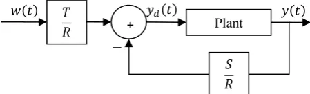
Controller (6) is structured as Fig. 1.

[image:2.595.63.288.573.641.2]

This control law represents a negative feedback with the transfer operator S R and a feedforward with the transfer operator T R . This is the general pole placement controller design where T R and S R are the poles should be specified.

Fig. 1: A general pole placement design controller

Taking system (4) and controller (5) to obtain the plant outputy t

 

:

 

BT

 

BR

 

y t w t v t

AR BS AR BS

 

 

 

 

 

d

AT BS

y t w t v t

AR BS AR BS

 

  (7)

The close-loop characteristic polynomial is thus become

c

ARBS A (8)

Expression (8) is solved by Diophantine equation. Only R and S can be determined by Diophantine equation. Other conditions must be introduced to also determine the polynomial T in the controller (5). The response from the command signalu_c is required to the output be described by the dynamics

 

 

m m m c

A y t B u t (9)

It then follows from output (7) that the condition below must be held:

m

c m

B

BT BT

AR BS A A

 

 (10)

This model following condition indicates that the response of the close-loop system to command signals is as specified by the model (9). Whether model-following can be achieved depends on the model, the system, and the command signal. If it is possible to make the error equal to zero for all command signals, then perfect model-following is achieved.

Condition (10) implies that there are cancellations of factors ofBTandA_c. Factor the 𝐵 polynomial as

BB B  (11) whereBis a monic polynomial whose zeros are stable and so well damped that they can be cancelled by the controller andBcorresponds to unstable or poorly damped factors that cannot be cancelled. It thus follows thatBmust be a factor ofB_m. Hence

'

m m

B B B (12)

Since B is cancelled, it must be a factor of A_c . Furthermore, it follows from condition (10) thatA_mmust also be a factor of A_c . The close-loop characteristic polynomial thus has the from

0

c m

A  A A B (13)

Since B is a factor if B and

c

A , it follows from expression (8) that it also dividesR. Hence

'

RR B (14)

And the Diophantine expression (8) reduces to

' '

0 m c

AR B S A A A (15) Introducing equation (12), (13) and (14) into equation (11) gives

' 0 m

T  A B (16)

Consider a discrete-time plant process described by the transfer function

0 1 2

1 2

b z b

B

A z a z a

 

  (17)

Let the desired close-loop system be

0 2

2

1 2

m m m

c

m m m

B b z b

A

A z a z a



 

  (18)

The controller is thus characterized by the polynomials Plant

𝑇 𝑅

𝑆 𝑅

+

𝑤 𝑡 𝑦𝑑 𝑡 𝑦 𝑡

1 0

b

R z

b

  (19)

1 1 2 2

0 0

m m

a a a a

S z

b b

 

  (20)

0 0

m

b

T z

b

 (21)

Process above shows a simple discrete-time example how to establish a controller by pole placement. Since the design method is purely algebraic, there is no difference between discrete-time and continuous-time controller.

2.2 U-Model

The U-model is a time-varying parameter polynomial which can present smooth non-linear object. Under a U mapping, the U-model outputu t



1



oriented polynomial below,

 



  

* , 1





y t  f  U t

 

*



y t



1 ,



,y t



n

 

,u t 2 ,



,u t



n



,



      









 

2









1 1 1 M 1

U t  const u t u t u t

(22) where U t



1



is assumed that it is equal toy_d

 

t .

Correspondingly, its regression equation is given as

 

M_{j 0 j}

  

j 1



y t 



_



t u t (23) where 𝑀 is the degree of model input (controller output)



1



u t , the time varying parameter vector

 



 

 



1

0

M M

t t t R



_





_ 

is a function of past inputs and output



u t



2 ,



u t



n

 

,y t1 ,



,y t



n





, and the parameters





0 L

  .

To work out u t



1



, root-solving algorithm is adopted to resolve as



1



_d

 

M_{j 0 j}

  

j 1



0

u t  





y t 



_  t u t 





(24) where is a root-solving algorithm, such as Newton-Raphson algorithm (Chong and Zak, 2013). A detailed analysis on the root solving issues has been presented (Zhu and Guo, 2002).

For a linear plant model,





 

 

 

0 1

1 yd t t

u t

t

 



  (25)

where₁

 

t is the coefficient associated with u t



1



(for linear time invariant models,

 

1 t

 is a constant).

 

0 t



(nonzero) is the summation of the rest of the terms in the linear model (Zhu and Guo, 2002).

The U-model is defined as a general linearized model from the nonlinear polynomial model through the conversion to the U-model (23) and then assigned with required poles through a linear feedback control algorithm (Zhu, Zhao and Zhang, 2015).

There is an example for expediently understanding the polynomial to the U-model conversion.

The polynomial model is

 



 





 





 



2

0.1 1 2 0.5 1 1

0.8 1 2

y t y t y t y t u t

u t u t

     

   (26)

And the U-model can be expressed as equation (23),

 

 

  



  

2



0 1 2 2 1

y t 



t 



t u t 



t u t (27) where ₀

 

t 0.1y t



1

 

y t2



,₁

 

t 0.8u t



2



,

and

 





2 t 0.5y t 1

    .

It is worthwhile to mention that for linear systems, the polynomial has only two main factors: ₀and₁.

The general linear controller is described as controller (5):

 

 

 

d

Ry t Tw t Sy t (28) By lettingy t

 

y_d

 

t , the designed U-model can be linked to the referencew t

 

as

 

 

 

d

c

T T

y t w t w t

R S A

 

 (29)

where polynomial A_c is the close-loop characteristic equation and specified in advance, that is

c

R S A (30)

To cancel the possible output offset in steady state, i.e., to make steady state error equal to zero at the controlled output, polynomialTis specified with

 

1

c

T A (31)

The key idea of the design is to specify the desired close-loop characteristic polynomial A_c , then resolve the polynomialsRandSthrough a Diophantine equation (Zhu and Guo, 2002). After the desired plant output

 

d

y t is

desired, the controller outputu t



1



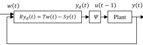
can be determined by resolving one of the root of the U-model (23), which the algorithm (24) and (25) has present. [image:3.595.308.545.538.612.2]

The whole framework of U-model in using linear pole placement approaches to design control systems with linear polynomial plant models is shown in Fig. 2.

Fig. 2: A U-model-based pole placement control system

3

Case Studies

3.1 Preparation

Consider two linear dynamic plant models for the computational experiments for two examples.

Plant 1:

 

















0.5 1 0.8 2

1 0.4 2

t y t y t

u t u t

y

   

    (32)

Plant 2:

 

2

0.5832 7.2610

0.4463 3.8730

s G s

s s

 

  (33)

𝑅𝑦𝑑 𝑡 = 𝑇𝑤 𝑡 − 𝑆𝑦 𝑡 𝛹 Plant

Specify the desired close-loop characteristic equation with

2

0.1761

1.3205 0.4966

c

z A

z z



  (34)

The control systems of two plants will be designed with both classical approach and U-model approach. Therefore provide computational comparisons.

3.2 Classical pole placement control Solution to Plant 1

The first step is to convert the linear dynamic plant (32) into the same formula as formula (17) using z-transform as

 

 

2

0.4 0.5 0.8

Y z z

U z z z

 

  (35)

And then observe plant (35). From plant (35), degA2

and deg B1are easily found out. The sampled data system has a zero in 0.4 and poles in1.1787 and 0.6787 .

From formula (17) and plant (35), b₀ 1,b₁ 0.4 ,

1 0.5

a  anda₂  0.8is determined.

From formula (18) and desired characteristic equation (34), bm₀ 0.1761 , am1 1.3205 and am20.4966 is determined.

As shown in formula (19), (20) and (21), R,TandScan be figured out:

1 0

0.4

b

R z z

b

   

1 1 2 2

0 0

0.8205 1.2966

m m

a a a a

S z z

b b

 

   

0 0

0.1761

m

b

T z z

b

  (36)

[image:4.595.307.545.282.602.2]

Therefore the whole controller can be determined by placing T R and S R as shown in Fig. 3.

Fig. 3: System response of Plant 1

Solution to Plant 2

The plant (33) is a continuous-time process. This can be regarded as a normalized model for a motor. The pulse transfer operator the sampling periodh0.5sis

 

₂ 0.5

0.8

z G z

z z

 

  (37)

From plant (37), degA2and degB1are found out. The sampled data system has a zero in 0.5 and poles in

0.5 1.4832 jand 0.5 1.4832 j.

From formula (17) and plant (37), b₀ 1 ,b₁ 0.4 ,

1 1

a  anda₂ 0.8is determined.

From formula (18) and desired characteristic equation (34), bm₀ 0.1761 , am1 1.3205 and am2 0.4966 is determined.

As the same step in solution to Plant 1 by classical pole placement control, R,TandSshould be figured out from formula (19), (20) and (21) again:

1 0

0.5

b

R z z

b

   

1 1 2 2

0 0

0.3205 0.3034

m m

a a a a

S z z

b b

 

   

0 0

0.1761

m

b

T z z

b

  (38)

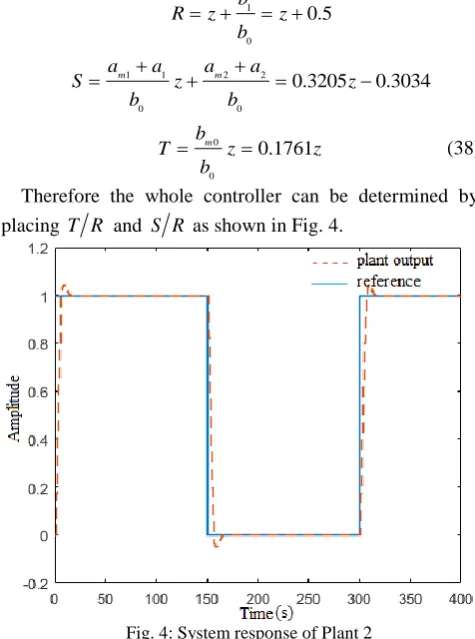
Therefore the whole controller can be determined by placing T R and S R as shown in Fig. 4.

Fig. 4: System response of Plant 2

3.3 U-model based pole placement control Solution to Plant 1

To achieve zero steady state error, specify Tby making the close-loop characteristic equation as

 

1 0.1761

c

TA  (39)

For the polynomialsRandS, specify 2

1 2 Rz r zr

0 1

Ss qs (40)

[image:4.595.51.287.512.706.2]

2 1 0.4966

r s 

1 0 1.3205

rs   (41)

To guarantee the computation convergence of the sequenceU t

 

, i.e. to keep the difference equation with stable dynamics, let r₁  0.9 and r₂ 0.009 . This assignment corresponds to the characteristic equation of

 

U t as



q0.89



q0.01



0. Then the coefficients in polynomial S can be determined from the Diophantine equation of (41) as

0 0.4205

s  

1 0.4876

s  (42)

Substituting the coefficients of the polynomialsRandS into the controller of (5) gives rise to





 









 





1 0.9 0.009 1

0.1761 1 0.4205

0.4876 1

d d

t y t y t

w t y t

y t

y

   

  

 

(43)

Therefore the controller outputu t

 

can be determined by solving the root in terms of equation









  



 

  







1

0 0

1 1

1

1 1

k k

M j

j j

M j

j j

u t u t

t u t U t

d t u t du t

 







  

  

 













(44)

𝑢𝑘+1 𝑡 − 1

= 𝑢𝑘 𝑡 − 1

− ∑ 𝜆̂𝑗 𝑡 𝑢

𝑗 _{𝑡 − 1 − 𝑈 𝑡} 𝑀

𝑗=0

𝑑[∑𝑀𝑗=0𝜆̂𝑗 𝑡 𝑢𝑗 𝑡 − 1 ] 𝑑𝑢 𝑡 − 1 ⁄

|

𝑢𝑗 𝑡−1 =𝑢_𝑘𝑗 𝑡−1

(44) The corresponding control-oriented model of is obtained from formula (25):

 

0

 

1

  

1



y t  t  t u t (45)

where

 













0 t 0.5y t 1 0.8y t 2 0.4u t 2

      

 

1 t 1

  (46)

Substitutingy t

 

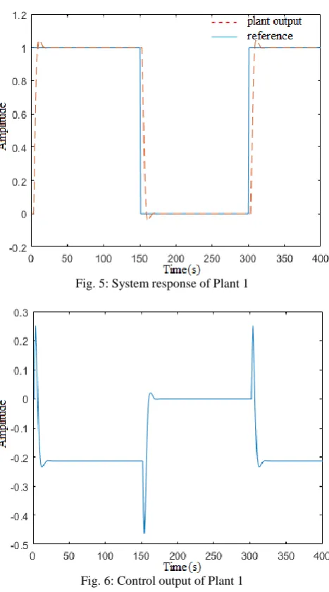
in equation (46) into (43), the output response of the designed U-model with assigned poles and steady state property is shown in Fig. 5, and the pole placement controller output is shown in Fig. 6 (Zhu and Guo, 2002).

Solution to Plant 2

Since the desired close-loop characteristic equation is the same one as solution to Plant 1 by U-model, there is no need to calculate the controller as equations (39) to (43). Utilize the same controller parameter and just figure out corresponding plant from U-model formula (25):

 

0

 

1

  

1



y t  t  t u t (47)

where

 













0 t y t 1 0.8y t 2 0.5u t 2

      

 

1 t 1

  (48)

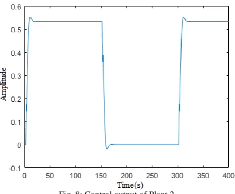
[image:5.595.84.546.84.755.2]

The output response of the designed U-model with assigned poles and steady state property is shown in Fig. 7, and the pole placement controller output is shown in Fig. 8.

Fig. 5: System response of Plant 1

Fig. 6: Control output of Plant 1

[image:5.595.312.546.97.518.2]

[image:6.595.51.287.56.251.2]

Fig. 8: Control output of Plant 2

3.4 Discussions

As shown above, the U-model derived from pole placement with modularisation, obtaining a root as the controller output from a polynomial equation. The simulation results of both classical pole placement and U-model’s demonstrate the same control performance achieved; however, the procedure of designing control system by U-model is much concise and generally applicable (once off design for all plant models) compared to classical pole placement (ad hoc design with each plant model). To explain the difference, further analysis is given below.

In U-model design, after specifying the desired close-loop characteristic polynomialA_c, polynomialsRandScan be resolved through Diophantine equation (which is shown in equation (30): R S A_c). As a classical approach in pole placement (Åström and Wittenmark, 1995), the corresponding relationship is given by expression (8):

c

ARBS AwhereAandBare the numerator polynomial and the denominator polynomial of a plant model, respectively, which indicate the classical design depending on the plant model. Without determining poles every procedure while plant is changed, the U-model set up a law of R,TandS.

Unlike pole placement method need to calculateR,T andSevery time when plant changing, U-model simplifies the routine to complete the design of control system. After the desired plant output y_d

 

t is designed, as solution to Plant 2 applies the same desired plant output in solution to Plant 1, the controller output u t



1



can be directly determined by resolving one of the roots of the U-model. That means, when desired close-loop characteristic

equation is set up, no matter how the plant model changed, the procedure from equations (39) to (43) is constancy.

This is one of theorems for U-model (Zhu and Guo, 2002): The u-model based pole placement design procedure does not depend on the plant model. Only the solution of the designed controller output involves in the plant model.

4

Conclusions

Even the proposition of U-model concept is to establish a framework which provides a generic prototype for using linear approaches to design control systems with smooth non-linear plants, U-model design still performs better in linear control system design. For linear control system design, the fundamental difference between classical approach and U-model approach lays in the design procedure. Classical approach is to design control system with plant model and controller together to find controller output, whereas U-model approach is design a general controller and then use plant models to find the controller output. Even the same control effect are obtained, U-model is superior in generality, concise, and teaching-learning. This study is the first paper to make such comparison with pole placement controller design, which should be also applicable to the other types of linear controllers.

For the future work, U-model methodology will be expanded to control non-minimum phase linear plants, stabilise unstable linear systems, and then compare with those type classical linear design approaches.

Acknowledgements

The first two authors are grateful to the partial studentship sponsored by the Engineering Modelling and Simulation Research Group, University of the West of England, Bristol, UK.

References

[1] E.K.P. Chong and S.H. Zak, An introduction to optimization (4th ed.). New York, NY: Wiley-Interscience, 2013. [2] K.J. Åström and B. Wittenmark, Adaptive Control, Addison

Wesley Boston, MA, USA, 1995.

[3] Q.M. Zhu, D.Y. Zhao and J. Zhang, A general U-block model-based design procedure for nonlinear polynomial control systems. International Journal of Systems Science, 1-10, 2015.

[4] Q.M. Zhu and L.Z. Guo, A pole placement controller for non-linear dynamic plants. Proceedings of the Institution of Mechanical Engineers, Part I: Journal of Systems and Control Engineering, 216(6): 467-476, 2002.