7
An Evolving Neuro-PSO-based Software Maintainability
Prediction
N. Baskar
Research Scholar
Department of Computer Science
Government Arts College
Udumalpet, Tamilnadu, India
C. Chandrasekar, PhD
Assistant Professor
Department of Computer Science
Government Arts College
Udumalpet, Tamilnadu, India
ABSTRACT
There are several issues related to the software maintenance but a more important critical one highlighted in this work is tracking over the behavior of software maintenance. This is because inferring the knowledge about the maintenance of software products in advance is really a difficult process which is pointed out by many researchers. Considering this issue the main purpose of this work is inspired based on Bio-Inspirational behavior-based optimization technique with an objective to predict software maintainability. In this paper, an attempt has been made to use subset of class-level object-oriented metrics in order to predicting software maintainability. Here, different subset of Object-Oriented software metrics have been considered to provide requisite input data to design the models for predicting maintainability using Neuro-Particle Swarm Optimization algorithm (NPSO). This technique is applied to estimate maintainability on dataset collected from two different case studies such as Quality Evaluation System (QUES) and User Interface System (UIMS). The performance parameters used in this technique has been evaluated based on the basis of Magnitude of Relative Error (MRE), Mean Magnitude of Relative Error (MMRE) and Prediction.
Keywords
PSO, NPSO, QUES, UIMS, MRE, MMRE
1.
INTRODUCTION
Software Maintainability is a design quality attribute which described as the ability of the system to undergo changes with a degree of ease, these changes could impact components, features and interfaces when changing the functionality or fixing errors [1]. Software maintainability is a key quality attributes of the software systems. Maintainability is one of the important quality attributes which can result in decreasing the cost of the software [2]. There is a belief that software with high quality is easy to maintain, so that minimum time and effort need to fix the faults and this will lead to decent maintainability and easily maintainable software [3].Developing software with no changes in future is really not possible and it is very sensitive to cost. The significant quality of developing software is it can be maintained easily and it leads to less resource usage both in terms of monetary and efforts .During the development phase, software metric plays an important role in controlling the cost of software maintenance. The earlier research work on software maintenance agreed that the metrics can be used for predicting the software maintainability and the reason for it is given below:
This will assist the project manager to evaluate the cost and productivity between other projects.
Usage of valuable resources can be well planned using the information provided by this prediction system.
Allocation of staff can also be efficiently handled by the manager with the aid of it.
The effort of further maintenance can be kept under control to reach the least maintenance cost.
It facilitates the software developers to recognize the quality of software therefore they can get better design and coding.
It facilitates practitioners to progress the systems software quality and thus minimize the maintenance costs.2.
RELATED WORK
Various methods have been proposed in the past to reduce the cost of software maintenance using object-oriented metrics. Here, few of those studies have been discussed.
John et al [4] presented a set of metrics are proposed to quantify and measure these attributes. The proposed complexity metrics are used to determine the difficulty in implementing changes through the measurement of method complexity, method diversity, and complexity density. The mostly employed approach for estimating software effort is the multivariate linear regression technique which has numerous shortcomings and motivates the exploration of many machine learning techniques. Marico et al [5] proposed a technique by employing an evolutionary algorithm to generate a decision tree tailored to a software effort data set provided by a large worldwide IT company. Their findings show that evolutionarily induced decision trees statistically outperform greedily induced ones, as well as traditional logistic regression.
The software complexity metric is one of the measurements that use some of the internal attributes or characteristics of software to know how they affect on the software quality. Yahya et al [6],covered some of more efficient software complexity metrics such as Cyclomatic complexity, line of code and Hallstead complexity metric. In their work they presented their impacts on the software quality.
8 In the study performed by Ruchika and Anuradha [11] an
attempt has been made to evaluate and examine the effectiveness of prediction models for the purpose of software maintainability using real life web-based projects. Three models using Feed Forward 3-Layer Back Propagation Network (FF3LBPN), General Regression Neural Network (GRNN) and Group Method of Data Handling (GMDH) are developed and performance of GMDH is compared against two others i.e. FF3LBPN and GRNN. With the aid of this empirical analysis, they suggest safely that software professionals can use OO metric suite to predict the maintainability of software using GMDH technique with least error and best precision in an object oriented paradigm. Probabilistic Neural Networks (PNN) is a feed forward neural network created by Ibrahim [12]. It is based on Bayesian network and Kernel Fisher discriminate analysis. In a PNN, the operations are organized into a multilayered feed forward network. First layer is input layer where one neuron is present for each independent variable. The next layer is the hidden layer. This layer contains one neuron for each set of training data. It not only stores the values of the each predictor variables but also stores each neuron along with its target value. Next is the Pattern layer. In PNN networks one pattern neuron is present for each category of the output variable. Last layer is output layer. At this layer weighted votes for each target category is compared and selected.PNN are known for their ability to train quickly on sparse datasets as it separates data into a specified number of output categories. The network produces activations in the output layer corresponding to the probability density function estimate for that category. The highest output represents the most probable category.
GRNN is a modification of Probabilistic Neural Network (PNN) for regression problems. It is a one-pass learning algorithm with highly parallel structure and provides a smooth transitions from one observed value to another even with sparse data in a multidimensional measurement space [13]. If the relationship between independent variables and dependent variables is very complex and not linear in nature, this modified form of regression is a perfect solution. It is very fast in learning and converges to the optimal regression surface as the number of samples becomes very large and allows learning from previous outcomes.
In an attempt to address this issue quantitatively, the main purpose of the work done in [14] is to propose use of few machine learning algorithms with an objective to predict software maintainability and evaluate them.
In the study done by Lov Kumara [15], empirically investigates the relationship of existing class level object-oriented metrics with a quality parameter i.e. maintainability. Here, different subset of Object-Oriented software metrics have been considered to provide requisite input data to design the models for predicting maintainability using hybrid approach of neural network and genetic algorithm.
3.
PROBLEM DEFINITION
If the result in the output layer is not ideal, the network will calculate the variation of errors and propagate errors back along the former route while correcting the weight. This process is repeated until it gets the satisfied result or it reaches the maximum number of iterations. Therefore, BP algorithm is also called as the back propagation of error. Although BP network has been widely used, it has serious flaws of slow convergence, prone to local minima, poor generalization and etc.
3.1 Solution Overview
The Neural Network models act as efficient predictors of dependent and independent variables due to its character in modeling where they possess the ability to model complex functions. In this approach, Particle Swarm Optimization algorithm is used for updating the weight during learning phase.
3.2 Proposed Methodology for
Maintainability Prediction using
Neuro-Particle Swarm Optimization
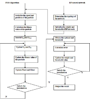
In this section the proposed Neuro-Particle Swarm Optimization (NPSO) algorithm is discussed in detail for predicting software maintainability. The PSO algorithm, when introduced into a BP neural network to optimize its initial weights and thresholds, is well suited for addressing some of the deficiencies caused by the randomness of the initial weights and thresholds of BP Neural Networks.
3.3 Back Propagation Neural Network
(BPNN)
During classification, a preprocessed data vector is first copied into input unit activations. Based on these values, and on the values of weights between input and hidden units, hidden units then calculate their activations. Based on hidden unit activations and hidden-to-output weights, output units calculate their activations. The network‟s chosen classification is then read from the output unit activations, which usually represents each class into which the input data
can be mapped [16].
Fig.1 Back Propagation Neural Network (BPNN)
3.4 Particle Swarm Optimization
Particle Swarm Optimization (PSO) is a population-based stochastic optimization technique inspired by bird flocking and fish schooling which was originally designed and introduced by Kennedy and Eberhart (1995) [17] and is based on iterations. The algorithmic following PSO starts with a population of particles whose positions represent the potential solutions for the studied problem and velocities are randomly initialized in the search space. In each iteration, the search for optimal position is performed by updating the particle velocities and positions. Also in each iteration, the fitness value of each particle‟s position is determined using a fitness function. The velocity of each particle is updated using two best positions, namely personal best position (pbest ) and global best position (gbest). The pbest is the best position the particle has visited, and gbest is the best position the swarm has visited since the first time step. A particle‟s velocity and position are updated as follows.
9
𝑋 𝑡 + 1 = 𝑋 𝑡0 + 𝑉 𝑡 + 1
(2)
Where, X and V are position and velocity of particle, respectively. W is inertia weight, c1 and c2 are positive constants, called acceleration coefficients which control the influence of pbest and gbest on the search process, P is the number of iterative generation, r1 and r2 are random values in the range [0, 1].
3.5 Global Best PSO
The global best PSO (or gbest PSO) is a method where the position of each particle is influenced by the best-fit particle in the entire swarm. It uses a star social network topology where the social information obtained from all particles in the entire swarm. In this method each individual particle has a current position in search space, a current velocity, and a personal best position in search space. The personal best position corresponds to the position in search space where particle had the smallest value as determined by the objective function, considering a minimization problem. In addition, the position yielding the lowest value amongst all the personal best is called the global best position which is denoted by gbest.
3.6 Local Best PSO
The local best PSO (or lbestPSO) method only allows each particle to be influenced by the best-fit particle chosen from its neighborhood, and it reflects a ring social topology . Here this social information exchanged within the neighborhood of the particle, denoting local knowledge of the environment [17 18].
3.7 Algorithm of PSO
The basic algorithm of particle swarm optimization is discussed in this subsection. The PSO is defined with following parameters where TPS is the number of total number of particles in the swarm and each of them have their own position represented using xposi in a given search space. Each particle has the capability to move with the velocity of Veli. During each iteration the particles are moved randomly to take their new position and they have their own best position traversed so far and it is stored and represented using pbest,i. The overall best known position from the whole swarm is denoted as gbest,i. randp and randg are uniformly distributed random numbers in the range [0,1], n is the number of dimensions.
For each particle i = 1, ..., TPS do the following:
Setup the initial position xposi of all particles within the lower boulo and upper bouup boundry position of search space.
Assign initially the known best position of particles as xposi
pbest,i<= xpos
If (fitness(pbest,i) < fitness(gbest,i.)) revise the swarm's best known position: gbest,i. ← pbest,i
Initialize the particle's velocity: Veli ~ U(-|bouup-boulo|, |bouup-boulo|)
Until a termination criterion is met ( number of iterations performed, or a solution with adequate objective function value is found), repeat:
For each particle i = 1, ..., TPS do:Pick random numbers: randp, randg ~ U(0,1) For each dimension d = 1, ..., n do:
Update the particle's velocity:
veli,d ← ω veli,d + φp randp (pbest,i-xposi,d) + φg randg (gbest,d-xposi,d)
Update the particle's position: xposi ← xposi + veli
If (fitness(xposi) < fitness(pbest,i)) do:Update the particle's best known position: pbest,i ← xi
If (fitness(pbest,i) < fitness(gbest,i)) update the swarm's best known position: gbest,i ← pbest,i
Nowgbest,iholds the best found solution.The coefficient ω controls the influence of the previous velocity on movement and it is called as inertia weight. And φp and φg are acceleration co-efficient‟s which lies between 0<= φp,φg<=2,the velocity vector may grow to infinity if the value of ω, φp and φg is not set correctly. This can be overcome by controlling the particle velocity to lie in [Velmin, Velmax].
3.8 Neuro-PSO Software
Maintenance-based Prediction Model
To optimize the Neural Network the PSO algorithm is used to initialize weight assignment between the network layers and initializing thresholds between neural nodes to perform global search within the solution space and to determine optimal initial weights and threshold at a fast convergence rate. The NPSO can utilize these initial weights and thresholds for both training and testing samples.
The procedure of the Neuro-PSO can be described as follows: 1. Initialize PSO parameters (population size, speed
and position of particles and iterations).
2. Determine the topology of the BP neural network and generate population particles. Each dimension of the particle corresponds to a neural network connection weight or threshold. So the dimension of the particle can be expressed as follows
Particles: Xi = (xi1,xi2,. . ..xiD)T, i = 1,2,. . .,n D = (IH) +(HO) +H+O
where I, H and O represent the number of nodes in the input layer, hidden layer and output layer of the BP neural network, respectively and D is Dimension.
3. Selecting fitness function, the inertia factor and the maximum iteration times. Randomly initializing the velocity and position of each particle.
4. Calculating fitness value of each particle by the following equation. The Pbest is selected as the positions of the current particles and gbest selected as the best position of all the particles. If current fitness value is lesser than the Pbfitness value, the current one replaces the Pb.
Particle fitness value = 2
1 1
)
(
1
ij N
i
i C j
j d
ij
y
y
N
d ij
y
Where,is real output of the network. yij is the predicted output of the network. N is the total number of training samples, C is the number of output neurons
10 as shown below, and then generate the new
particles. If velocity or position of particle is beyond the boundary, the velocity or position should be reset randomly.
vel(t+1) = (ω* vel(t)) + (φp* randp * (pbest(t) –
xpos(t)) + (φg * randg * (gbest(t) – xpos(t))
xpos(t+1) = xpos(t) + vel(t+1)
6. Evaluate each new particle‟s fitness value. If the ith particle‟s new position is better than Pbest, Pbest is selected as the new position of the ith particle. If the best position of all new particles is better than gbest, then gbest is updated.
7. If the maximal iteration times or the fitness values are met, stop the iteration, and the positions of particles represented by gbest are the optimal best solution. Otherwise, the process is repeated from step3.
8. Taking the weights and threshold values which is optimized by PSO as the initial parameters, the BP network makes autonomous learning.
The training phases of the NPSO are as follows:
9. Initialize the network. The network structure, expected output and learning rate are determined according to the sample characteristics. The PSO algorithm optimization is used to derive the optimal individual solution for the initial weight value and threshold of the network.
10. Input the training sample and calculate the output of the network layers.
11. Calculate the learning error of the network.
12. Correct the connection weight values and thresholds of the layers.
13. Judge whether the error satisfies the expectation requirements and whether the number of iterations has reached the set training limit. If either condition is met, then the training ends. Otherwise, the iterative learning process continues.
Fig.2 Work Flow of Neuro-PSO based Software Maintenance Prediction
3.9 Maintenance Dataset Description
[image:4.595.163.473.279.621.2]In this paper, the maintenance effort data is obtained from Object-Oriented software data sets published by Li and Henry [19]. The Software Systems are User Interface System (UIMS) and Quality Evaluation System (QUES) are chosen for computing the maintenance effort. The softwares system, UIMS have 39 and QUES have 69 classes. The data was collected by the author over the past three years. The maintainability of software is measured by the number of lines changed per class.
Table 1 Dataset Attribute Description
Depth of Inheritance Tree (DIT)
It is defined as the longest path from root to leaf node. The deeper the hierarchy the higher is the complexity of the predecessor
Weighted Method Complexity (WMC)
It is the number of local methods in a class
Number of Children (NOC)
It is the number of subclasses a class contains
Coupling between Objects (CBO)
11
Lack of Cohesion of Methods (LCOM)
It is based on the numbers of pairs of methods that shared references to instance variables
Messaging Passing Coupling (MPC)
This metric measures the numbers of messages passing among objects of the class
Response for Class (RFC)
Number of Distinct Methods and Constructors invoked by a Class
Data Abstraction Coupling (DAC)
This metric measures the number of instantiations of other classes within the given class
Number of Methods (NOM)
This metric is used to calculate the average count of all class operations per class
Size 1 Number of Semicolons per class
Size 2 Number of Methods plus number of
attributes
CHANGE
Change is used as the dependent variable in this study and is defined as the number of lines modified, added or deleted from version 1 to version 2 of the software
3.10 Worked Out Example
Step 1: Initialize the input and network architecture as
shown in figure 3.
Fig.3 Initialization of Input in ANN
Step 2: Assigning weights to all of the synapses. These weights are selected randomly (based on Gaussian distribution) since it is the first time forward propagating. The initial weights will be between 0 and 1. It is depicted in figure 4.
Fig.4
:
Initial weights assign to each synapsesStep 3: Sum the product of the inputs with their corresponding set of weights to arrive at the first values for the hidden layer. The weights are considered as measures of influence the input nodes have on the output.
1 * 0.4 + 1 * 0.9 = 1.3 1 * 0.8 + 1 * 0.2 = 1.0 1 * 0.5 + 1 * 0.3 = 0.8
Put these sums smaller in the circle, because they‟re not the final value as shown in the figure 5.
Fig.5 Calculating weights for each hidden nodes
Step 4: To get the final value, and apply the activation function to the hidden layer sums. The purpose of the activation function is to transform the input signal into an output signal and is necessary for neural networks to model complex non-linear patterns that simpler models might miss. In this work sigmoid function is used for activation.
S(1.3) = 0.78583498304 S(1.0) = 0.73105857863 S(0.8) = 0.68997448112
Add that to neural network as hidden layer resultsas shown in the figure 6.
Fig.6 Finding hidden layer results and final output
Step 5: Then, sum the product of the hidden layer results with the second set of weights (also determined at random the first time around) to determine the output sum.
0.79 * 0.5 + 0.73 * 0.3 + 0.69 * 0.9 = 1.235 Finally apply the activation function to get the final output result.
S(1.235) = 0.7746924929149283
4.
EXPERIMENTAL RESULT AND
DISCUSSION
4.1 The network topology of neuron
networks
In this study, the BP neuron network has three layers including one hidden-layer. The neural networks models are trained with 11 neurons as input data, while 6 neurons for the hidden layer, and 1 neuron for output layer. The neuron transferring function in hidden-layer is sigmoid function in matlab represented as tansig, and that in output-layer is purely
1
1
12 linear is represented as purelin. And the training function is
traingdm. The training error precision is 0.0001.
4.2 Parameters of PSO
The parameters of PSO were selected as follows. The initial location and velocity of search point is randomly generated between [-1, 1]; the maximum velocity of particles
is 0.5; the population size is 40; the maximum times of iteration is 30000; the accelerated coefficients c1 =2.3, c2=1.8; the inertia weight is gradually decreased from 0.90 to 0.40 in order to reduce the influence of past velocity, and the particle dimension is 19.
Table 2 Statistics of class UIMS
Dit noc mpc Rfc Lcom Dac Wmc Nom size2 size1 Change
Min 0 0 1 2 1 0 0 1 1 4 2
Max 4 8 12 101 31 21 69 40 61 439 289
Mean 2.15 0.95 4.31 23.21 7.49 2.67 11.38 11.38 13.97 105.31 46.82
Median 2 0 3 17 6 1 5 7 9 74 18
Standard
Deviation 0.90 2.01 3.41 20.19 6.11 4.22 15.90 10.21 13.47 115.34 71.89
Table 3 Statistics of class QUES
dit Noc Mpc Rfc Lcom dac wmc nom size 2 size 1 Change
Min 0 0 2 17 3 0 1 4 4 115 6
Max 4 0 42 156 33 25 83 57 82 1009 217
Mean 1.91 0.00 17.87 54.65 9.20 3.45 15.09 13.45 18.07 277.61 64.507246
Median 2 0 17 40 5 2 9 6 10 216 52
Standard
Deviation 0.54 0.00 8.36 33.05 7.35 3.97 17.29 12.12 15.37 173.67 43.410362
Table 2 and 3 shows the calculated value of Min, Max, Median and Standard deviation values of the two software systems (UIMS and QUES). In this analysis, the derivative of inheritance metric „NOC‟ in UIMS has all its 39 classes and QUES software product has all its 69 classes with NOC values zero.
This indicates that there are no immediate sub-classes of a class in the class hierarchy and hence NOC is not considered in computing maintainability in this analysis.
4.3 Measures used to analyze software
maintainability
Various measures have been suggested to analyse the accuracy of prediction of a model. All these measures are based on the predicted value and the actual value. The actual and predicted values of the proposed model is implemented using matlab code.
The Evaluation metric used in this work are described below: Magnitude of Relative Error (MRE): It is measured by taking the absolute value of the difference between the actual value and the predicted value as given by Kitchenham [20]. The formula for this measure is:
MRE =
e
Actualvalu
alue
predictedv
e
Actualvalu
Mean Magnitude of Relative Error (MMRE): MMRE is the mean of MRE as proposed by Conte, Dunsmore and Shen [21]. The formula for this measure is:
MMRE =
N
I
I
MRE
1
Pred: Pred is measured by the predicted values whose MRE is less than or equal to a specified value. This was proposed by Fentom [22]. The formula for this measure is given in the Pred() equation, where k is the number of predicted values which are lesser than or equal to the specified value, q is the specified value and N is the total number of cases.
[image:6.595.310.547.575.722.2]Pred(q) =
N
K
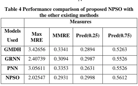
Table 4 Performance comparison of proposed NPSO with the other existing methods
Measures
Models
Used
Max
MRE MMRE Pred(0.25) Pred(0.75)
GMDH 3.42656 0.3341 0.2894 0.5263
GRNN 2.40739 0.3094 0.2987 0.5526
PNN 3.05611 0.3353 0.2631 0.5526
NPSO 2.02547 0.2931 0.2998 0.5612
13 result. From the table it is observed that the Max MRE is
[image:7.595.315.551.72.219.2]obtained by GMDH whereas the NPSO has the least error value. The least error value obtained by this proposed work shows that its performance is higher in prediction of accurate outcomes.
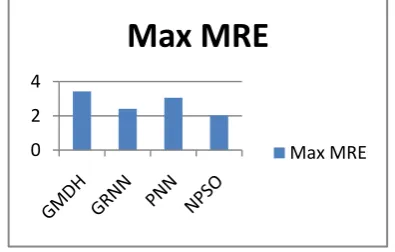
Fig.7 Performance comparison based on MAX MRE
[image:7.595.68.266.125.251.2]In this work the class used for prediction is change. The MRE value is computed based on computing the difference between actual values of class attribute change for each record which is compared with the predicted outcome of the NPSO for each instances and dividing with the actual value. The maximum MRE value of each technique is compared and shown in the figure above. The proposed NPSO shows better performance by producing minimum error value next to that GRNN holds the place and the worst case is produced by GMDH.
Fig.8 Performance comparison based on MMRE
[image:7.595.60.275.372.503.2]In this work each instance of maintenance dataset MRE values obtained from the above-mentioned formula is summed together for whole dataset and produces mean magnitude of relative error. The optimal search quality of the particle swarm optimization with neural network optimized the prediction of software maintenance cost.
Fig.9 Performance comparison on the Prediction value 0.25
Fig.10 Performance Comparison based on predicted value 0.75.
The output of the result predicted by NPSO is compared with the actual output of the class attribute change for the given prediction value 0.25 and 0.75. The whole prediction values cannot be listed in this paper, so running example for two prediction values are taken. The number of times the prediction value 0.25 and 0.75 produced by the proposed model is taken into the count and total number of instances is divided with that count. The proposed model produces more number of correct prediction values than the other existing approaches because of its heuristic learning‟s and correcting technique.
5.
CONCLUSION
In this work four different machine learning algorithms are used for the purpose of prediction of software maintainability. The goal of this study is to construct suitable model using machine learning algorithm for the prediction of object-oriented software maintainability which is not only easy to apply but also could reduce the prediction errors to minimum. This study quantitatively evaluates the prediction capability of three neural network- based algorithms. It compares the three existing models namely GMDH, GRNN PNN with proposed Neuro-PSO (NPSO) on the basis of four measures: MRE, MMRE, Pred (0.25) and Pred (0.75) from which it is concluded that out of the four models, Neuro-PSO gives the best results and the least value for MMRE and maximum values for Pred (0.25) and Pred (0.75). This technique concludes that Neuro-PSO is the best model for prediction of software maintainability. Future work may contain additional quantitative studies on different datasets so as to ensure the full potential of Neuro-PSO. Another direction of study may suggest combining of Neuro-PSO model with other data mining models to develop a prediction model which would more accurately predict software maintainability.
6.
REFERENCES
[1] Kan, S.H., Metrics and models in software quality engineering. 2002: Addison-Wesley Longman Publishing Co., Inc.
[2] Coleman, D., et al., Using metrics to evaluate software system maintainability. Computer, 1994. 27(8): p. 44-49. [3] Singh, B. and S.P. Kannojia, A Model for Software
Product Quality Prediction. 2012
[4] John Michura, Miriam A. M. Capretz, and Shuying Wang, Extension of Object-Oriented Metrics Suite for Software Maintenance, Software Engineering, Volume 2013 (2013)
0
2
4
Max MRE
Max MRE
0.25
0.3
0.35
GMDH GRNN PNN NPSO
MMRE
MMRE
0.24
0.26
0.28
0.3
0.32
Pred(0.25)
Pred(0.25)
0.5
0.52
0.54
0.56
0.58
GMDH GRNN PNN NPSO
Pred(0.75)
[image:7.595.57.279.589.721.2]14 [5] Marcio P. Basgalupp , Rodrigo C. Barros , Duncan D.
Ruiz, Predicting software maintenance effort through evolutionary-based decision trees, SAC '12 Proceedings of the 27th Annual ACM Symposium on Applied Computing pp 1209-1214, March 2012
[6] Yahya Tashtoush, Mohammed Al Maolegi, Bassam Arkok, The Correlation among Software Complexity Metrics with Case Study, International Journal of Advanced Computer Research (ISSN (print): 2249-7277 ISSN (online): 2277-7970) Volume-4 Number-2 Issue-15 June-2014 414
[7] M. Thwin and T. Quah, "Application of neural networks for software quality prediction using object oriented metrics," Journal of Systems and Software, vol. 76, no. 2, pp. 147-156, 2005.
[8] S. Misra, "Modeling design/coding factors that drive maintainability of software systems,”Software Quality Journal, vol. 13, no. 3, pp. 297-320, 2005.
[9] A Kaur, K Kaur, R Malhotra, “Soft Computing Approaches for Prediction of Software Maintenance Effort”, International Journal of Computer Applications), vol 1, no. 16, pp : 0975 – 8887, 2010.
[10]MO. Elish and KO. Elish “Application of TreeNet in predicting object-oriented software maintainability: A comparative study,” European Conference on Software Maintenance and Reengineering, pp 1534-5351, DOI 10.1109/CSMR
[11]Ruchika Malhotra, Anuradha Chug, Application of Group Method of Data Handling model for software maintainability prediction using object oriented systems, International Journal of System Assurance Engineering and Management, ISSN 0975-6809Volume 5Number 2, 2014
[12]M.M. Ibrahiem, E.l. Emary and S. Ramakrishnan, “On the Application of Various Probabilistic Neural Networks in Solving Different Pattern Classification Problems”, World Applied Sciences Journal , vol. 4, no. 6, pp. 772-780, 2008, ISSN 1818- 4952.
[13]Martin CL , Applying a general regression neural network for predicting development effort of short-scale programs. Neural Comput Appl, 20:389–401, 2011 [14]Ruchika Malhotra and Anuradha Chug, Software
Maintainability Prediction using Machine Learning Algorithms, Software engineering : an international Journal (SeiJ), Vol. 2, no. 2, September 2012
[15]Lov Kumara, Debendra Kumar Naikb, Santanu Ku. Rathc, Validating the Effectiveness of Object-Oriented Metrics for Predicting Maintainability, Third International Conference on Recent Trends in Computing (ICRTC‟ 2015)
[16]Eberhart, R. C. and R. W Dobbins (1990). Neural Network PC Tools: A Practical Guide. Academic Press, San Diego, CA.
[17]Eberhart, R. C. and Kennedy, J. A new optimizer using particle swarm theory., Proceedings of the Sixth International Symposium on Micromachine and Human Science, Nagoya, Japan. pp. 39-43, 1995
[18] Kennedy, J. and Eberhart, R. C. Particle swarm optimization. Proceedings of IEEE International Conference on Neural Networks, Piscataway, NJ. pp. 1942-1948, 1995
[19]Li, W. and S. Henry, Object-oriented metrics that predict maintainability. Journal of systems and software, 1993. 23(2): p. 111-122.
[20]. B.A. Kitchenham, L.M. Pickard, S.G. MacDonell, M.J. Shepperd,” What accuracy statistics really measure,” IEEE ProceedingsSoftware vol. 148, no. 3, pp 81–85, 2001.
[21] S. Conte, H. Dunsmore, and V. Shen,” Software engineering metrics and models”. Book, Menlo Park, CA: Publisher: Benjamin-Cummings publishing co., ISBN: 0-8053-2162-4, 1986.
[22]N.E. Fentom, S.L. Pfleeger, “Software metrics: A Rigorous and practical approach, second edition,” PSW publishing Company, 1997.