Asymptotic Behavior and Stability of Stochastic SIR Model with Variable Diffusion Rates

(1)

http://www.scirp.org/journal/am ISSN Online: 2152-7393

ISSN Print: 2152-7385

DOI: 10.4236/am.2017.88080 Aug. 7, 2017 1031 Applied Mathematics

Asymptotic Behavior and Stability

of Stochastic SIR Model with

Variable Diffusion Rates

Xianhua Xie

1

, Li Ma

1,2

, Jingfei Xu

1*

1_{Key Laboratory of Jiangxi Province for Numerical Simulation and Emulation Techniques, Gannan Normal University, Ganzhou,} China

2_{College of Mathematics and Econometrics, Hunan University, Changsha, China}

Abstract

In this paper, we propose random fluctuation on contact and recovery rates in deterministic SIR model with disease deaths in nonparametric manner and derive a new stochastic SIR model with distributed time delay and general diffusion coefficients. By analysis of the introduced model, we obtain the suf-ficient conditions for the regularity, existence and uniqueness of a global solu-tion by means of Lyapunov funcsolu-tion. Moreover, we also investigate the sto-chastic asymptotic stability of disease free equilibria and endemic equilibria of this model. Finally, we illustrate our general results by applications.

Keywords

SIR Model, Regularity, Lyapunov Function, Stochastic Asymptotic Stability

1. Introduction

SIR models are the foundation for a large number of compartmental models in mathematical epidemiology which classify the population into three classes: Susceptible, Infected and Removed (see [1]-[19]). Generally, these models admit two types of equilibrium: disease free and endemic equilibrium. If the disease free equilibrium is asymptotically stable, it implies the disease dies out. If the endemic equilibrium is asymptotically stable, it implies the disease persists in the population at the equilibrium level.

In 1976, Hethcote [13] considered the following deterministic SIR model with disease deaths:

*Corresponding author. How to cite this paper: Xie, X.H., Ma, L.

and Xu, J.F. (2017) Asymptotic Behavior and Stability of Stochastic SIR Model with Variable Diffusion Rates. Applied Mathe-matics, 8, 1031-1044.

https://doi.org/10.4236/am.2017.88080

Received: May 12, 2017 Accepted: August 4, 2017 Published: August 7, 2017 Copyright © 2017 by authors and Scientific Research Publishing Inc. This work is licensed under the Creative Commons Attribution International License (CC BY 4.0).

http://creativecommons.org/licenses/by/4.0/

(2)

DOI: 10.4236/am.2017.88080 1032 Applied Mathematics

( )

( ) ( )

(

( )

)

( )

( ) ( ) (

) ( )

( )

,

.

S t S t I t K S t

I t S t I t I t

R t I t R t

β µ

β µ α

α µ

 ′ = − + −

 _′ ₌ ₋ ₊



 ′ = −



(1)

In Equation (1), S t

( ) ( ) ( )

,I t ,R t denote the number of the individuals susceptible to the disease, of infected members and of members who have been removed from the population, respectively. The model (1) is based on the following assumptions:

i) The population considered has a constant size K, that is, S t

( ) ( )

+I t +R t

( )

=K for all t;

ii) Births and deaths occur at equal rates µ in K. All the newborns are susceptible. µ is called a daily death removal rate;

iii) β is the daily contact rate, i.e., the average number of contacts per infective per day. A contact of an infective is an interaction which results in infection of the other individual if it is susceptible;

iv)

α

_{is the daily recovery removal rate of the infective. Of course,}

, , R

β µ α_∈ +_.

In [8], Beretta and Takeuchi pointed out that when a susceptible vector is infected by a person, there is a time τ>0 during which the infectious agents

develop in the vector and it is only after that time that the infected vector becomes itself infectious, and proposed the following model

( )

( ) (

)

(

( )

)

( )

( ) (

)

(

) ( )

( )

0

d ,

,

h

S t S t f s I t s s K S t

I t S t f s I t s s I t

R t I t R t

β µ

β µ α γ

α µ

 ′ = − − + −



 ′ = − − + +

 

′ = −

 

∫

(2)

where f s

( )

is a non-negative function which is square integrable on

[ ]

0,h and satisfies

( )

0 d 1, 0 d ,

h h

f s s= sf s s< +∞

∫

(3)

and the non-negative constant h is the time delay, βS t

( )

∫

₀hf s I t

( ) (

−s

)

ds can

be viewed as the force of infection at time t.

In fact, all infectious diseases are subject to randomness in terms of the nature of transmission. Recently, Tornatore et al. [16] investigate the dynamics of system (2) by perturbing the functional contact rates and modified (2) as:

( )

( ) (

)

( )

( ) (

)

( )

( ) (

)

(

) ( )

( )

( ) (

)

( )

0 0

d d d d d

d d d d

d ,

h h

S t S t f s I t s s S t t S t f s I t s s W t

I t S t f s I t s s I t S t f s I t s s W t

R t I t R t

β µ µ σ

β µ α σ

α µ

 _{= −} ₋ ₋ ₊  ₋ ₋

 

  

 ₌_ ₋ ₋ ₊ _₊ ₋

 __ __



 = −



∫

(4)

(3)

DOI: 10.4236/am.2017.88080 1033 Applied Mathematics stochastic SIR model with deaths and varying contact and recovery rates, where the introduced model covers general diffusion coefficients (functional contact and recovery rates).

In order to make the SIR system (2) more realistic, we consider the case of

( ) ( )

( )

S t +I t +R t ≤K and we perturbed the deterministic system (2) by a white noise and obtained a stochastic counterpart by replacing the rates

β

by

( ) ( ) ( )

(

)

1

( )

1

d

, ,

d

W t

F S t I t R t

t

β+ and α by

(

( ) ( ) ( )

)

2

( )

2

d

, ,

d

W t

F S t I t R t

t

α+ ,

and hence we modify the SIR system (2) as the following model:

( )

( ) (

)

(

( )

)

( )

( ) (

)

( ) ( ) ( )

(

)

( )

( ) (

)

(

) ( )

( )

( ) (

)

( ) ( ) ( )

(

)

( )

( ) (

)

(

( ) ( ) ( )

)

( )

( ) (

)

(

( ) ( ) ( )

)

( )

0 0

1 1

0 0

1 1 ₀ 2 2

2 2

0

d d d d

, , d ,

d d d

, , d d , , d

d d , , ,

h h

h

S t S t f s I t s s K S t t S t f s I t s s

F S t I t R t W t

I t S t f s I t s s I t S t f s I t s s

F S t I t R t W t f s I t s sF S t I t R t W t

R t I t R t f s I t s sF S t I t R t dW t

β µ

β µ γ α

α µ

 _{= −} ₋ ₊ ₋  ₋ ₋

 

  



× 

 ₌_ ₋ ₋ _{+ +} _₊ ₋

 __ __



 _× ₋ ₋



 ₌ ₋ ₊ ₋



∫



(5)

where α β µ, , ,K have the same meaning as model (2), W ti

( )(

i=1, 2

)

are real

Wiener processes and i.i.d which defined on a filtered complete probability space

(

Ω, ,F F

( )

t t≥0,P

)

. Here, we introduce other two new general stochastic terms: functions F ii

(

=1, 2

)

which are locally Lipschitz continuous defined on

(

)

{

3

}

, , : 0, 0, 0, .

S I R S I R S I R K

= ∈ ≥ ≥ ≥ + + ≤

 

Besides, there are deaths due to disease the total population size may vary in time so that we always assume the total population size is less than K in the context, where K represents a carrying capacity. Note that if we consider the population size is a constant K and the disease-related death rate γ =0, besides

we also take F t1

( )

=F t2

( )

=σ (where σ is a positive constant), the system (3) becomes the model which has been discussed in [16]. In [16], Tornatore proved the stability of disease-free equilibrium under some restricted conditions. However, they didn’t consider the dynamics of the endemic equilibrium. It is of great importance from a theoretical point of view to investigate the stability of the endemic equilibrium.

In this paper, we mainly study the stochastic SIR model (5) with distributed delay which has more general diffusion coefficients than model (4)’s. By means of averaged Itô formula and Lyapunov function, we obtain the sufficient conditions for the regularity, existence and uniqueness of a global solution. Furthermore, we also investigate the stochastic asymptotic stability of disease free equilibria and the dynamics of endemic equilibria which has not been discussed in [16].

(4)

DOI: 10.4236/am.2017.88080 1034 Applied Mathematics to ensure the global stochastic asymptotic stability of disease free equilibrium in SIR model (5), besides we also consider the stochastic asymptotic stability of endemic equilibrium in Section 5. Finally, we illustrate our general results by applications.

2. Some Preliminary Definition and Lemmas

At first, we recall the notation of regularity of continuous time stochastic processes as introduced in [10]. Let  ⊂ d

(

d≥1

)

be a fixed closed domain.

For Simplicity, we only consider deterministic domains  ⊂ 3 _{in this} exposition.

Definition 1. A continuous time stochastic process

{

X t t

( )

, ≥0

}

is called

regular on  (or invariant with respect to ) if

( )

(

)

0 : 1,

t P X t

∀ ≥ ∈ =

otherwise irregular with respect to  (or not invariant with respect to ). Consider the d-dimensional stochastic differential equation of the form

( )

(

( )

)

(

( )

)

( )

dX t = f X t t, dt+g X t t dW t, ,

(6) with an initial value X t

( )

0 =X t0,0≤ ≤ < ∞t T where :

[

0,

]

d d

f  × t T →

and :

[

0,

]

(

1

)

d d m

f  × t T → × m≥ are Borel measurable,

{

( )

}

0 t t

W= W t _≥ is an

m

 -valued random variable.

Definition 2. The infinitesimal generator



associated with the SDE (6) is given by

( )

(

( ) ( )

T

)

2

1 , 1

1

, , , .

2

d m

i

ij

i i i j i j

f x t g x t g x t

t = x = x x

∂ ∂ ∂

= + +

∂

∑

∂

∑

∂ ∂



Lemma 2.1. (Regularity Theorem [10]) Let  and n be open sets in d



with

1, , and ,

n n n n

n

+

⊆ ⊆ =

_

     

and suppose f and g satisfy the existence and uniqueness conditions for

solutions of (6) on each set

{

( )

t x, :t>t x0, ∈n

}

. Suppose there is a nonnegative continuous function V:

[

t T0,

]

+

× →

  with continuous partial derivatives and satisfying V ≤cV for some positive constant c and t>t₀, x∈.

Moreover, if

( )

0, \

inf , as ,

n

t t x> ∈  V x t → ∞ n→ ∞

then P X

(

0∈

)

=1 for any X0 independent of σ

( )

W , that is to say the stochastic process

{

X t t

( )

, ≥0

}

is called regular on . Regularity on 

implies boundedness, uniqueness, continuity and Markov property of the strong solution process X of SDE (6) with X

( )

0 =X₀, and X t

( )

∈ for all t>0

(a.s.).

Definition 3. The equilibrium solution *

(5)

( )

0 *

0 0 ,

lim sup s X 0,

X x t s

P X t

→ ≤ <∞

 _≥ ₌

 

 

where Xs X, 0

( )

t denotes the solution of (6) satisfying X s

( )

=X0 at time

t

≥

s

.

x of the SDE (6) is stochastically asymptotically stable (stable in probability) if it is stochastically stable and

( )

(

0

)

* 0

* ,

lim lim _{s X} 1.

t X x

P X t x

→∞

→ = =

x of the SDE (6) is said to be globally stochastically asymptotically stable (stable in probability) if it is stochastically stable and for every X0 and every s

( )

(

0

)

* ,

lim _{s X} 1.

t

P X t x

→∞ = =

Lemma 2.2. ([4]) Assume that f and g satisfy locally Lipschitz-continuous

and satisfy linear growth condition and they have continuous coefficients with respect to t.

1) Suppose that there exists a positive definite function 2,1

(

[

)

0,

h

V∈C U × t ∞ ,

where

{

*

}

:

d h

U = ∈x  x−x <h for

h

>

0

, such that

( )

, 0, 0, h.

V x t ≤ ∀ ≥t t x U∈



Then the equilibrium solution *

x of (6) is stochastically stable.

2) In addition, if

V

is descresent (that is to say there exists a positive definite

function V1 such that V x t

( )

, ≤V x1

( )

for all x U∈ h ) and V x t

( )

, is negative definite, then the equilibrium solution *

x is stochastically asymptotically stable.

3) If the assumptions of part (2) hold for a radially unbounded function

[

)

(

)

2,1

0,

d

V∈C  × t ∞ defined everywhere then the equilibrium solution * x is globally stochastically asymptotically stable.

3. Existence, Uniqueness and Regularity of Stochastic SIR

Model Solution

Theorem 3.1. Let

(

S t

( ) ( ) ( )

0 ,I t0 ,R t0

)

=

(

S I R0, 0, 0

)

∈ =D

(

)

{

3

}

, , , 0 : 0, 0, 0,

S I R ∈ t≥ S≥ I≥ R≥ S+ + ≤I R K , and

(

S I R0, 0, 0

)

be independent of σ_-algebraσ

(

W t t

( )

, ≥0

)

. Then, under the condition (A) or (B)

a)

∫

₀hf s I t

( ) (

−s

)

ds≤LI t

( ) (

L>0

)

;

b)

∫

₀hf s I t

( ) (

−s

)

ds≤I t

( )

+R t

( )

;

the stochastic process

{

(

S t

( ) ( ) ( )

,I t ,R t

)

,t≥t0

}

governed by Equation (5) is regular on  ; i.e. we have P

(

S t

( ) ( ) ( )

,I t ,R t

)

∈

)

=1 for all t≥0 .

(6)

(

)

( ) (

)

(

)

( ) (

)

(

)

0 0 d

, , d

h

S f s T t s s K S

b S I R S f s I t s s I

I R

β µ

β α µ γ

α µ  ₋ ₋ ₊ ₋      =_ − − + + _  ₋     

∫

and the diffusion term

(

)

( ) (

)

( ) (

)

1 0 2 0 2

d 0 0

, , d 0 .

0 0

h

SF f s I t s s

B S I R S f s I t s s IF

IF ₋ ₋      =_ − − _      

∫

Let open domains

(

)

{

}

: , , : e n e , en n e , en n e ,n , .

n S I R S K I K R K S I R K n

− − − − − −

= < < − < < − < < − + + ≤ ∈

 

Since Equation (5) is well-defined on  and n , and the coefficients

(

, ,

)

b S I R , B S I R

(

, ,

)

are locally Lipschitz-continuous and satisfy linear growth

condition on , then there exists a unique, bounded and Markovian solution up to random time τ

( )

_ (or τ

( )

n ), where τ

( )

 (or τ

( )

n represents the random time of the first exit of stochastic process

(

S t

( ) ( ) ( )

,I t ,R t

)

from the domain  (or n ), started in

(

S t

( ) ( ) ( )

,I t ,R t

)

=

(

S s

( ) ( ) ( )

,I s ,R s

)

=

(

S I R0, 0, 0

)

∈ (or (S I R0, 0, 0)∈n) at the initial time s∈

[

t0,∞

)

. To ensure the solution regular, we only prove that P

(

τ

( )

 = ∞ =

)

1. a.s. Now, we use

function 2

( )

V∈C  defined on  via

(

, ,

)

ln ln

(

)

ln

(

) (

)

ln

(

)

,

V S I R = −S S+ −I I+ K−S − K−S + K−R − K−R

and assume that EV S I R

(

, ,

)

< ∞. For

(

S I R, ,

)

∈, we have V S I R

(

, ,

)

≥4

and for

(

S I R, ,

)

∈ \ n, we have

(S I R, ,inf)∈ \ _nV S I R

(

, ,

)

>2n+2, forn∈. (7)

Define



as infinitesimal generator as in Definition 2, then calculate

(

)

(

( ) (

)

(

)

( ) (

)

(

)

( ) (

)

(

)

(

)

(

)

(

)

( ) (

)

(

)

0 0

2 2 2

2

2 2

1 2 2

0

2 2 2

2 2

2 2 2

0

, , d

d

1

d , , 2

2

1

, , 2

2 1 1 d h h h h V

V S I R S f s I t s s K S

S V

S f s I t s s I R

R

V V V

S f s I t s s F S I R

S I

S I

V V V V

I F S I R I

I R I

I R

S f s I t s s K S

K S S

β µ

β α µ

α γ µ

β µ ∂ = − − + − ∂ ∂  +_ − + − ∂  ∂ ∂ ∂  + − _ − + _ ∂ ∂ ∂ ∂    ∂ ∂ ∂  ∂ +  − _{∂ ∂} + − + + __∂ ∂ ∂      = − − + − _ − _ −  

∫



( ) (

)

(

)

( ) (

)

(

)

(

)

(

)

0 2 2 2

1 2 2 2

0

1 1

d 1 1

1 1 1 1

d , ,

2

h

S f s I t s s I R

I K R

S I

K S

β   α µ  

(7)

(

)

(

)

(

)

( ) (

)

( ) (

)

(

)

( ) (

)

( ) (

)

( ) (

)

(

)

(

)

( ) (

)

(

)

(

)

( )

2 2

2 2 2

0 0 0 0 2 2 1 0 2 2 1 0 2 2 0

1 1 1 1

, , 1

2 d d 1 d d 1

d , ,

2

d , ,

1 2 1 2 h h h h h h h

I F S I R I

I

I _K _R

S f s I t s s K S

f s I t s s

K S S

S f s I t s s S f s I t s s

I

I R

I R f s I t s s F S I R

K R K R

f s I t s s F S I R

S

I

f s I t

α γ µ

β _µ

µ β

β β α γ µ

α _α µ _µ

  _ _   + + − + + _ − _  ₋  _ _   − − − = + + − − − + − − − + + + + − − + + − − − − + +

∫

_∫

∫

(

)

(

)

(

)

(

)

( ) (

)

(

)

(

)

( ) (

)

(

)

(

)

2 2 2 2 2 2 1 0 2 2 2 2 2 0 2

d , ,

( )

d , ,

1

2 ( )

d , ,

1

. 2

h

s s F S I R

I

K R

S

K S

I

α γ µ − − + + − − + − − +

∫

In view of the condition (A) that

∫

₀hf s I t

( ) (

−s

)

ds≤LI t

( )

, and hence we have

(

)

( ) (

)

( ) (

)

( )

(

)

(

)

( )

(

)

(

)

0 0

2 2 2

1 2

, ,

2 2 2

1 2

, ,

, , 3 d d 2

3 , , , , sup 2 3 2 3 , , , , . sup 2 h h

S I R

V S I R f s I t s s S f s I t s s

R LK F S I R LF S I R

LI SI R

LK F S I R LF S I R

µ β β α

γ µ

µ β β α γ µ

∈ ∈ ≤ + − + − +   + + + _ + _   ≤ + + + + +   + _ + _  

∫

  

If we take

( )

(

)

(

)

2 2 2

1 2

, ,

1 3

0 < 3 2 sup , , , , ,

4 S I R 2

c µ βLI βSI α γ µR LK F S I R LF S I R

∈

  

≤  + + + + + +  + 

 

  

therefore V S I R

(

, ,

)

≤cV S I R

(

, ,

)

due to V S I R

(

, ,

)

≥4 for

(

S I R, ,

)

∈.

In what follows, to show that P

(

τ

( )

 = ∞ =

)

1, i.e., P

(

τ

( )

 < =t

)

0. Now,

introduce a new function 1,2

(

[

)

,

W∈C s ∞ × by

(

,

(

, ,

)

ec t s( )

(

, ,

)

W t S I R = − − V S I R ,

where c is defined as above. And hence

(

)

(

)

( )

₍

₎

₍

₎

, , , e c t s , , , , 0,

W t S I R = − − _−cV S I R + V S I R _≤

 

since V S I R

(

, ,

)

≤cV S I R

(

, ,

)

. Denote τn: min=

{

τ

( )

n ,t

}

and apply

averaged Itô formula, we have

( )

₍

_{( ) ( ) ( )}

₎

( ) ( )

₍

_{( ) ( ) ( )}

₎

( )

₍

_{( ) ( ) ( )}

₎

e , ,

e e , ,

e , , ,

n

n c t

n n n

c s c t s

n n n

c t s

n n n n

E V S I R

E W S I R

τ τ

τ τ τ

τ τ τ τ

(8)

( )

₍

_{( ) ( ) ( )}

₎

( )

₍

_{( ) ( ) ( )}

₎

( ) ( ) ( )

(

)

(

)

( )

₍

_{( ) ( ) ( )}

₎

( )

₍

_{( ) ( ) ( )}

₎

( )

₍

₎

0 0 0

e , , ,

, , , d

e , , ,

e , ,

e , , .

n

c t s

n n n n

c t s

s

c t s

E W S I R

EW s S s I s R s

E W x S x I x R x x

EW s S s I s R s

EV S s I s R s

EV S I R

τ

τ τ τ τ

−

  

= _ _ __

  

= _ _ _



+ _

 

≤ _ _

 

= _ _

≤

∫



Using this fact and Equation (7), one can estimates

( )

(

)

(

( )

)

(

)

(

)

( )

(

( )

)

(

( )

)

(

( )

)

( )

(

)

( )

(

)

( )

(

)

( )

(

)

, , \

0 0 0

, , \

0 0 0

0

, ,

e

inf , ,

, ,

e

inf , ,

, ,

e 0 as ,

2 2

n

n n

n

n n

n n n

c t

t S I R

c t

S I R

c t

P t P t P t E I t

V S I R

E

V S I R I

EV S I R V S I R

EV S I R

n n

τ τ

τ

τ τ τ

−

< ∈

−

∈ −

≤ < ≤ < = < = <

 

 

≤

 

 

≤

≤ → → ∞

+

 

  

for all fixed t∈

[

s,+∞

)

, because of the appearance of the function I

( )

. . Thus

( )

(

)

(

( )

n

)

0

P τ  < =t P τ  < =t for

(

S I R0, 0, 0

)

∈ and t≥t0 , that is,

( )

(

n

)

1

P τ  = ∞ = .

Then it proves the regularity and the global existence of the solution

( ) ( ) ( )

(

S t ,I t ,R t

)

∈ and by means of Lemma 2.1 under the condition of (A),

we also derive the uniqueness and continuity of the solution.

Similarly the above discussions, we only need to take the function V S I R

(

, ,

)

as S−lnS+

(

K−S

)

−ln

(

K−S

)

, and we can also obtain the same results under the condition of (B). Here, we omits the details.

This completes the proof of Theorem 3.1. 

Remark 3.1. Because I= = =S R 0 are undefined in the domain . In what

follows, we distinguish three cases to investigate the solution of these special situations.

1) If S=0, then the system (5) will reduce to

( )

(

) ( )

)

( ) (

)

(

( ) ( )

)

( )

(

( )

)

( ) (

)

(

( ) ( )

)

0

d d d , d ,

h

I t K I t t f s I t s sF I t R t W

R t I t R t t f s I t s sF I t R t W

µ α γ µ

α µ

 ₌ ₋ _{+ +} ₋ ₋

 

 = − + −



∫

(8)

with intial condition

(

I R0, 0

)

∈D1=

{

(

I R,

)

:I>0,R>0,I+ ≤R K

}

. By using the similar analysis, we know that the above SDE is regular which implies there exists a unique global solution on D1;

2) If I=0, then the system (5) will reduce to an ODE

( )

(

( )

)

( )

d d ,

S t K S t t

R t R t t

µ µ

 = −

 

= −

(9)

DOI: 10.4236/am.2017.88080 1039 Applied Mathematics with intial condition

(

S R0, 0

)

∈D2 =

{

(

S R,

)

:S>0,R>0,S+ ≤R K

}

. By using the theory of ODE, we know that the above ODE is regular which implies there exists a unique global solution on D2;

3) If R=0, then the system (5) will become

( )

(

( )

( ) (

)

(

( )

)

( )

(

( ) ( )

)

( )

(

( )

( ) (

)

(

) ( )

)

( )

( ) (

)

(

( ) ( )

)

0

d d d

( ) , d ,

d d d

d , d ,

h

S t S t f s I t s s K S t t

f s I t s ds F S t I t W

I t S t f s I t s s I t t

S t f s I t s s F S t I t W

β µ

β α µ

 _{= −} ₋ ₊ ₋

 

− − ×

 

 = − − +



 ₊ ₋ _×



∫

(10)

with intial condition

(

S I0, 0

)

∈D3 =

{

( )

S I, :S>0,I>0,S+ ≤I K

}

. By using the similar analysis, we know that the above SDE is regular which implies there exists a unique global solution on D3.

4. Global Stochastic Asymptotic Stability

of Disease Free Equilibrium

Theorem 4.1. Assume that ₀hf s I t

( ) (

s

)

ds I t

( )

K

α γ µ β + +

− ≤

∫

for all fixed

[

,

)

t∈ ∞s , then the disease free equilibrium solution

(

S I R1, ,1 1

) (

= K, 0, 0

)

of Equation (5) is globally stochastically stable on .

Proof. Notice that the assumption ₀hf s I t

( ) (

s

)

ds I t

( )

K

α γ µ β + +

− ≤

∫

for all

fixed t∈ ∞

[

s,

)

, and hence one can estimates that there exists a positive constant

C which satisfies

( ) (

)

(

) ( )

0 d

h

Kβ

∫

f s I t−s s≤ ≤C α γ µ+ + I t for all fixed

[

,

)

t∈ ∞s . Introduce a Lyapunov function

(

)

1

(

)

2

, , .

2

V S I R = S+ + −I R K +CI

Just note that the infinitesimal generator



satisfies

(

)

(

( ) (

)

(

)

(

)

( ) (

)

(

)

(

)

(

)

(

)(

)

(

( ) (

)

(

)

(

) (

)

( ) (

)

(

)

(

)

(

( ) (

)

(

)

0

2

0 2

2

0

2

, , d

d

h

V S I R S f s I t s s K S S I R K

S f s I t s s I S I R K

I R S I R K C S f s I t s s I

K S I R K S I R I C S f s I t s s

MI I RI

K S I R C f s I t s s I S

K C I I R

β µ

β α γ µ

α µ β α γ µ

µ γ β

α γ µ γ γ

µ β γ

γ α γ µ γ γ

= − − + − + + −

+ − − + + + + −

+ − + + − + − − + +

= − − − − + − − − + −

− + + − −

= − − − − + − −

+_ − + + _ − −

∫



(

)

2 2

,

I

K S I R I RI

µ γ γ

≤ − − − − − −

(11)

then V S I R

(

, ,

)

becomes negative definite on , and hence it completes the

(10)

DOI: 10.4236/am.2017.88080 1040 Applied Mathematics Remark 4.1. As we known, the basic reproduction number R0 is one of the most important parameters in epidemiology, which reflects the expected number of secondary infections produced when one infected individual entered a fully susceptible population. If R0<1 then the outbreak will disappear, on the other hand, if R0 >1 then the epidemic will spread a population. In this context, the basic reproduction number of the SIR model is 0

K

R β

α γ µ =

+ + .

5. Stochastic Asymptotic Stability of Endemic Equilibrium

If R0>1 and F S I Ri

(

2, 2, 2

) (

=0 i=1, 2

)

, then there exists a unique endemic equilibrium solution

(

S I R2, 2, 2

)

for the model (5), where

(

)

(

) (

)

2 2 2

0 0

0

, , , 1 , 1

, 1 , 1 .

K K

S I R

K

R R

R

α γ µ µ β α β

β β α γ µ β α γ µ

µ α

β β

 + +    

=  _{+ +} −   _{+ +} − 

   

 

 

=_ − − _

 

Theorem 5.1. The endemic equilibrium solution,

(

S I R2, 2, 2

)

of the Equation(5) is stochastically asymptotically stable on

(

)

{

S I R, , :S 0,I 0,R 0,S I R K

}

= > > > + + ≤

 under the assumption of R0>1

for some F S I Ri

(

, ,

)

such that F S I Ri

(

2, 2, 2

)

=0 and satisfies G S I R

(

, ,

)

≤0, where

(

)

(

)

(

)

(

)

( ) (

)

(

)

(

)

( ) (

)

(

)

(

)

( ) (

)

(

)

(

)

2 2

2 2 2 2

2 2 2

2 ₀ 2 2

2

2 2

1 0

2 2 2 0

, ,

d

d , ,

2

d , , ,

2

h

G S I R S I R S I R I I

S I R S I R

a S S f s I t s s b S S b R R

a

b

µ γ

β µ µ

= − + + − − − − −

+ + + +

− − − − − − −

+ −

∫

(12)

and

(

)(

)

(

)

(

( ) (

)

(

)(

)

(

)

(

( ) (

)

(

)(

)

(

)

(

( ) (

)

(

)(

)

(

)

(

( ) (

)

2 2 2 ₀ 2

2

2 2 2 ₀ 2

2

2 2 2 ₀ 2

0, if 0, d 0;

, if 0, d 0;

0, if 0, d 0,

h

s S S I I S S f s I t s s I

S S I I S S f s I t s s I

a

K

a S S I I S S f s I t s s I

S

S S I I S S f s I t s s I

γ β

 > − − > − − − >

 

− − < − − − <

  = 

 > − − < − − − >

 

= − − > − − − <



∫

(13)

( )

(

)

(

)(

)

(

)(

)

2 2

, ,

2 2

inf , if 0;

, if 0.

S I R _S _I _R S S R R

b

S S R R

K

γ α γ α

∈

 ₋ ₋ _>

 _{+ +}

 = 

 ₋ ₋ _<





(14)

Proof. It is a fact that the endemic equilibrium solution of system (5) exists if 0 1

(11)

(

)

(

) (

)

(

)

(

)

2 2 2 2 2 2

2 2 2

2 2

, , ln

,

2 2

S I R

V S I R S I R S I R S I R

S I R

a b

S S R R c

+ +

= + + − + + − + +

+ +

+ − + − +

on , where a and

b

are defined as Equations ((13) and (14)), c is an

arbitrary positive constant. An elementary computation leads to V >0 for any

point

(

S I R, ,

)

∈, and we have

(

)

( ) (

)

(

)

(

)

( ) (

)

(

)

( ) (

)

( ) (

)

(

)

(

)

(

)

2 2 2

2 0

2 2

2 2 2

1 2

0 0

2 2 2

0

2 2 2

2

, , d 1

d , , d

2 2 d 1 1 . h h h h

S I R

V S I R S f s I t s s K S a S S

S I R

a b

S f s I t s s F S I R f s I t s s F

S I R

S f s I t s s I

S I R

I R b R R

S I R

β µ

β α γ µ

α µ + +     = −_ − + − __ − + − _   + +      + ×_ − _ + _ − _     + +     +_ − − + + __ − _   + +  + +   + − _ − + − _ + +  

∫



From the following formulas and the definitions of a,

b

can help to

simplify 

(

S I R, ,

)

i) µ

(

K− − −I S R

)

−γI= −µ

(

S+ + −I R S2− −I2 R2

) (

−γ I−I2

)

;

ii)

( ) (

)

(

)

(

)

( ) (

)

(

( ) (

)

(

)

0

2 ₀ 2 ₀ 2 2

d

d d ;

h

h h

S f s I t s s K S

S S f s I t s s S f s I t s s I S S

β µ

β β µ

− − + −

= − − − − − − − −

∫

iii) α β µ β+ + = S2;

iv) αI−µR=α

(

I−I2

)

−µ

(

R−R2

)

. Then

(

)

(

)

(

)

( ) (

)

(

( ) (

)

(

)

( ) (

)

( ) (

)

[

]

(

)

(

)(

)

2 2 2

2 2

2 2 2

0 0

2 2

2 2 2

1 2

0 0

2 2

2 2 2 2

2 2

1

d d

d ( , , ) d

2 2

h h

S I R

V K S I R I a S S S S

S I R

f s I t s s S f s I t s s I S S

a b

S I R S I R I I

S I R S I R

S S I I

S I R

µ γ β

β µ µ γ γ + +   =_ − − − − __ − _+ − _− − + +    × − − − − − −      + _ − _ + _ − _     = − + + − − − − − + + + + − − − − + +

∫



(

)(

)

(

)

( ) (

)

(

)

(

( ) (

)

( ) (

)

(

)

( ) (

)

[

]

(

)

(

)

(

) (

)

(

)

(

)(

)

2 2 2

2 ₀ 2 2 ₀ 2

2 2

2 2 2

1 2

0 0

2 2

2 2 2 2

2

2 2 2 2

2

2 2 2

d d

d , , d

2 2

( )

h h

I I R R

S I R

a S S f s I t s s a S S S f s I t s s I

a b

S I R S I R I I

S I R S I R

a S S b R R I I R R

b I I R R b R R a S

γ

β β

µ γ

µ α µ

α µ µ

− − + + − − − − − − −     + _ − _ + _ − _     ≤ − + + − − − − − + + + + − − + − _ − − − _ + − − − − −

∫

(

)

(

)

( ) (

)

(

)

( ) (

)

(

)

( ) (

)

2 2 2 2

2 ₀ 2

2 2

2 2 2

1 2

0 0

d

d , , d .

2 2

h

h h

S

a S S f s I t s s b R R

a b

(12)

(

, ,

)

0

V S I R =

 if and only if

(

S I R, ,

) (

= S I R2, 2, 2

)

and by the given condition one can obtain V <0 on \

(

S I R₂, ₂, ₂

)

. Therefore V S I R

(

, ,

)

is negative definite on  for some suitable F S I Ri

(

, ,

)

. Then Lemma 2.2 (ii)

leads to the stochastically asymptotical stability of the endemic equilibrium with 0 1

R > and for some suitable functions F S I Ri

(

, ,

)

such that F S I Ri

(

, ,

)

satisfies Equation (12) and F S I Ri

(

2, 2, 2

)

=0. 

6. Example

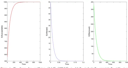
In this section, we visualize our results with some simulation to confirm them. Due to the difficulty of the research on the drawing of the disease equilibrium point, many scholars have not given the relevant examples. Along this clue, we only give the figures of the disease-free equilibrium point (Figure 1). We consider the special case 1

( ) (

)

( )

0f s I t−s ds=I t

∫

which only satisfies the condition of Theorem 4.1 ₀hf s I t

( ) (

s

)

ds I t

( )

K α γ µ

β + +

− ≤

∫

, that is, Kβ 1

α γ µ+ + < , and

hence we can obtain the disease free equilibrium solution

(

S I R1, ,1 1

) (

= K, 0, 0

)

of Equation (5) is globally stochastically stable on . In the simulation, the parameters are chosen as follows

1000, 1 / 75 0.013, 52, 52, 0.05.

K= µ= = α = γ = β=

Acknowledgements

Special thanks to the anonymous referees for very useful suggestions. The research has been supported by the Natural Science Foundation of China

Figure 1. The disease free equilibrium

(

S I R, ,

) (

= 1000,0,0

)

is globally stochastically asymptotically stable since

0.97 1

Kβ Kβ

[image:12.595.54.539.429.689.2]

(13)

DOI: 10.4236/am.2017.88080 1043 Applied Mathematics (11361004). Xian-Hua Xie is supported by the Bidding Project of Gannan Normal University (16zb01). all of the authors are supported by the Key Laboratory of Jiangxi Province for Numerical Simulation and Emulation Techniques.

Conflict of Interests

The authors declare that the study was realized in collaboration with the same responsibility.

Competing Interests

The authors declare that they have no competing interests regarding the publication of this paper.

Authors Contributions

All of the authors, XHX, LM and JFX contributed substantially to this paper, participated in drafting and checking the manuscript, and have approved the version to be published.

References

[1] Allen, E.J., Allen, L.J.S. and Schurz, H. (2005) A Comparison of Persistence-Time Estimation for Discrete and Continuous Stochastic Population Models That Include Demographic and Environmental Variability. Mathematical Biosciences, 196, 14- 38. https://doi.org/10.1016/j.mbs.2005.03.010

[2] Allen, E.J. (1999) Stochastic Differential Equations and Persistence Time for Two Interacting Populations. Dynamics of Continuous, Discrete and Impulsive Systems, 5, 271-281.

[3] Arciniega, A. and Allen, E. (2004) Shooting Methods for Numerical Solution of Stochastic Boundary-Value Problems. Stochastic Analysis and Applications, 22, 1295-1314. https://doi.org/10.1081/SAP-200026465

[4] Arnold, L. (1974) Stochastic Differential Equation. Wiley, New York.

[5] Bartholomew, D.J. (1982) Stochastic Models for Social Processes. Wiley, New York. [6] Bartlett, M.S., Gower, J.C. and Leslie, P.H. (1960) A Comparison of Theoretical and

Empirical Results for Some Stochastic Population Models. Biometrika, 47, 1-11

https://doi.org/10.1093/biomet/47.1-2.1

[7] Beretta, E., Kolmanovskii, V. and Shaikhet, L. (1998) On the General Structure of Epidemic System, Global Asymptotic Stability. Computers & Mathematics with Ap-plications, 12, 677-694. https://doi.org/10.1016/0898-1221(86)90054-4

[8] Beretta, E. and Takeuchi, Y. (1995) Global Stability of an SIR Epidemic Model with Time Delays. Journal of Mathematical Biology, 33, 250-260

https://doi.org/10.1007/BF00169563

[9] Carletti, M. (2002) On the Stability Properties of a Stochastic Model for Phage- Bacteria Interaction in Open Marine Environment. Mathematical Biosciences, 175, 117-131. https://doi.org/10.1016/S0025-5564(01)00089-X

[10] Gard, T.C. (1988) Introduce to Stochastic Differential Equations. Marcel Dekker, Basel.

(14)

https://doi.org/10.1016/S0895-7177(03)90029-X

[12] Hanson, F.B. and Tuckwell, H.C. (1981) Logistic Growth with Random Density In-dependent Disasters. Theoretical Population Biology, 19, 1-11.

https://doi.org/10.1016/0040-5809(81)90032-0

[13] Hethcote, H.W. (1976) Qualitative Analyses of Communicable Disease Models. Mathematical Biosciences, 28, 335-356.

https://doi.org/10.1016/0025-5564(76)90132-2

[14] Schurz, H. (2001) Moment Attractivity, Stability and Contractivity Exponents of Stochastic Dynamical Systems. Discrete and Continuous Dynamical Systems— Series A, 7, 487-515. https://doi.org/10.3934/dcds.2001.7.487

[15] Schurz, H. (2007) Modelling Analysis and Discretization of Stochastic Logistic Equ-ations. International Journal of Numerical Analysis and Modeling, 4, 180-199. [16] Tornatore, E., Buccellato, S.M. and Vetro, P. (2005) Stability of a Stochastic SIR

System. Physica A: Statistical Mechanics and its Applications, 354, 111-126.

https://doi.org/10.1016/j.physa.2005.02.057

[17] Zhang F., Gao, S., Liu, Y., et al. (2016) Dynamics of a Nonautonomous SIR Model with Time-Varying Impulsive Release and General Nonlinear Incidence Rate in a Polluted Environment. Applied Mathematics, 7, 681-693.

https://doi.org/10.4236/am.2016.77062

[18] Zhang, Y., Chen, S., Gao, S., et al. (2017) A New Non-Autonomous Model for Mi-gratory Birds with Leslie-Gower Holling-Type II Schemes and Saturation Recovery rate. Mathematics and Computers in Simulation, 132, 289-306.

https://doi.org/10.1016/j.matcom.2016.07.015

[19] Zhao, Y. and Yuan, S.L. (2017) Optimal Harvesting Policy of a Stochastic Two-Species Competitive Model with Lévy Noise in a Polluted Environment. Physica A: Statis-tical Mechanics and its Applications, 477, 20-33.

https://doi.org/10.1016/j.physa.2017.02.019

Submit or recommend next manuscript to SCIRP and we will provide best service for you:

Accepting pre-submission inquiries through Email, Facebook, LinkedIn, Twitter, etc. A wide selection of journals (inclusive of 9 subjects, more than 200 journals)

Providing 24-hour high-quality service User-friendly online submission system Fair and swift peer-review system

Efficient typesetting and proofreading procedure

Display of the result of downloads and visits, as well as the number of cited articles Maximum dissemination of your research work