warwick.ac.uk/lib-publications
Original citation:
Kosmidis, Ioannis. (2014) Improved estimation in cumulative link models. Journal of the
Royal Statistical Society: Series B (Statistical Methodology), 76 (1). pp. 169-196.
Permanent WRAP URL:
http://wrap.warwick.ac.uk/98828
Copyright and reuse:
The Warwick Research Archive Portal (WRAP) makes this work of researchers of the
University of Warwick available open access under the following conditions.
This article is made available under the Creative Commons Attribution 3.0 (CC BY 3.0) license
and may be reused according to the conditions of the license. For more details see:
http://creativecommons.org/licenses/by/3.0/
A note on versions:
The version presented in WRAP is the published version, or, version of record, and may be
cited as it appears here.
©2013 The Author. Royal Statistical Society published by John Wiley & Sons Ltd
This is an open access article under the terms of the Creative Commons Attribution License, which permits use, distribution and reproduction in any medium, provided the original work is properly cited.
This article was first published online on 3 July 2013, under a subscription licence. This article has since been made Open Access and the licence statement has been updated in this version in June 2014.
1369–7412/14/76169 76,Part1,pp.169–196
Improved estimation in cumulative link models
Ioannis Kosmidis
University College London, UK
[Received April 2012. Revised January 2013]
Summary.For the estimation of cumulative link models for ordinal data, the bias reducing adjusted score equations of Firth in 1993 are obtained, whose solution ensures an estimator with smaller asymptotic bias than the maximum likelihood estimator. Their form suggests a parameter-dependent adjustment of the multinomial counts, which in turn suggests the solution of the adjusted score equations through iterated maximum likelihood fits on adjusted counts, greatly facilitating implementation. Like the maximum likelihood estimator, the reduced bias estimator is found to respect the invariance properties that make cumulative link models a good choice for the analysis of categorical data. Its additional finiteness and optimal frequentist prop-erties, along with the adequate behaviour of related asymptotic inferential procedures, make the reduced bias estimator attractive as a default choice for practical applications. Furthermore, the estimator proposed enjoys certain shrinkage properties that are defensible from an experimental point of view relating to the nature of ordinal data.
Keywords: Adjusted counts; Adjusted score equations; Ordinal response models; Reduction of bias; Shrinkage
1. Introduction
In many models with categorical responses the maximum likelihood estimates can be on the boundary of the parameter space with positive probability. For example, Albert and Anderson (1984) derived the conditions that describe when the maximum likelihood estimates are on the boundary in multinomial logistic regression models. Although there is no ambiguity in reporting an estimate on the boundary of the parameter space, as is for example an infinite estimate for the parameters of a logistic regression model, estimates on the boundary can
(a) cause numerical instabilities to fitting procedures,
(b) lead to misleading output when estimation is based on iterative procedures with a stopping criterion and, more importantly,
(c) cause havoc with asymptotic inferential procedures, and especially with those that depend on estimates of the standard error of the estimators (e.g. Wald tests and related confidence intervals).
The maximum likelihood estimator in cumulative link models for ordinal data (McCullagh, 1980) also has a positive probability of being on the boundary.
1.1. Example 1
As a demonstration consider the example in Christensen (2012a), section 7. The data set in Table 1 comes from Randall (1989) and concerns a factorial experiment for investigating factors
Address for correspondence: Ioannis Kosmidis, Department of Statistical Science, University College London, Gower Street, London, WC1E 6BT, UK.
170 I. Kosmidis
Table 1. Wine tasting data (Randall, 1989)
Temperature Contact Responses on the following bitterness scale:
1 2 3 4 5
Cold No 4 9 5 0 0
Cold Yes 1 7 8 2 0
Warm No 0 5 8 3 2
Warm Yes 0 1 5 7 5
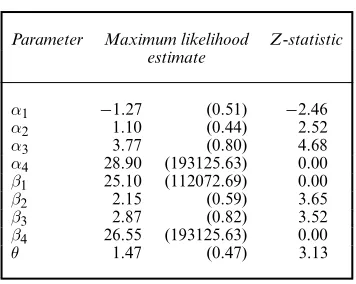
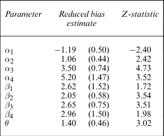
Table 2. Maximum likelihood estimates for the parameters of model (1), the corresponding es-timated standard errors (in parentheses) and the values of theZ-statistic for the hypothesis that the corresponding parameter is 0
Parameter Maximum likelihood Z-statistic estimate
α1 −1.27 (0.51) −2.46
α2 1.10 (0.44) 2.52
α3 3.77 (0.80) 4.68
α4 28.90 (193125.63) 0.00
β1 25.10 (112072.69) 0.00
β2 2.15 (0.59) 3.65
β3 2.87 (0.82) 3.52
β4 26.55 (193125.63) 0.00
θ 1.47 (0.47) 3.13
that affect the bitterness of white wine. There are two factors in the experiment: temperature at the time of crushing the grapes (with two levels, ‘cold’ and ‘warm’) and contact of the juice with the skin (with two levels ‘yes’ and ‘no’). For each combination of factors two bottles were rated on their bitterness by a panel of nine judges. The responses of the judges on the bitterness of the wine were taken on a continuous scale in the interval from 0 (‘none’) to 100 (‘intense’) and then they were grouped correspondingly into five ordered categories, 1, 2, 3, 4 and 5.
Consider the partial proportional odds model (Peterson and Harrell, 1990) with
log
γ
rs 1−γrs
=αs−βswr−θzr .r=1,: : :, 4;s=1,: : :, 4/, .1/
estimated standard errors and the corresponding values for theZ-statistics for the hypothesis that the respective parameter is 0 are extracted from the software output and shown in Table 2. At those values for the maximum likelihood estimator the maximum absolute log-likelihood derivative is less than 10−10 and the software correctly reports convergence. Nevertheless, an immediate observation is that the absolute values of the estimates and estimated standard errors for the parametersα4,β1andβ4are very large. Actually, these would diverge to∞as the
stop-ping criteria of the iterative fitting procedure used become stricter and the number of iterations allowed increases.
For model (1) interest usually is on testing departures from the assumption of proportional odds via the hypothesisβ1=β2=β3=β4. Using a Wald-type statistic would be adventurous
here because such a statistic explicitly depends on the estimates ofβ1,β2,β3andβ4. Of course,
given that the likelihood is close to its maximal value at the estimates in Table 2, a likelihood ratio test can be used instead; the likelihood ratio test for the particular example has been carried out in Christensen (2012a), section 7.
Furthermore, the current example demonstrates some of the potential dangers that are involved in the application of cumulative link models in general; the behaviour of the individual Z-statistics—being essentially 0 for the parametersβ1andβ4in this example—is quite typical of
what happens when estimates diverge to∞. The values of theZ-statistics converge to 0 because the estimated standard errors diverge much faster than the estimates, irrespective of whether or not there is evidence against the individual hypotheses. This behaviour is also true for individual hypotheses at values other than 0 and can lead to invalid conclusions if the output is interpreted naively. More importantly, the presence of three infinite standard errors in a non-orthogonal (in the sense of Cox and Reid (1987)) setting like the current setting may affect the estimates of the standard errors for other parameters in ways that are difficult to predict.
An apparent solution to the issues that are mentioned in example 1 is to use a different estimator that has probability 0 of resulting in estimates on the boundary of the parameter space. For example, for the estimation of the common difference in cumulative logits from ordinal data arranged in a 2×kcontingency table with fixed row totals, McCullagh (1980) described the generalized empirical logistic transform. The generalized empirical logistic transform has smaller asymptotic bias than the maximum likelihood estimator and is also guaranteed to give finite estimates of the difference in cumulative logits because it adjusts all cumulative counts by 12. However, the applicability of this estimator is limited to the analysis of 2×ktables, and particularly in estimating differences in cumulative logits, with no obvious extension to more general cumulative link models, such as that in example 1.
172 I. Kosmidis
parameters themselves. Secondly, the choice of the tuning parameter is usually performed through the use of an optimality criterion and cross-validation. Hence, the properties of the re-sultant estimators are sensitive to the choice of the criterion. For example, criteria like the mean-squared error of predictions, classification error and log-likelihood that have been discussed in le Cessie and van Houwelingen (1992) will each produce different results, as was also shown in le Cessie and van Houwelingen (1992). Furthermore, the resultant ridge estimator is sensitive to the type of cross-validation that is used. For example,k-fold cross-validation will produce different results for different choices ofk. Lastly, standard asymptotic inferential procedures for perform-ing hypothesis tests and constructperform-ing confidence intervals cannot be used by simply replacperform-ing the maximum likelihood estimator with the ridge estimator in the associated pivots. For these reasons, ridge estimators can only offer anad hocsolution to the problem.
Several simulation studies on well-used models for discrete responses have demonstrated that bias reduction via the adjustment of the log-likelihood derivatives (Firth, 1993) offers a solution to the problems relating to boundary estimates; see, for example, Mehrabi and Matthews (1995) for the estimation of simple complementary log–log-models, Heinze and Schemper (2002) and Bullet al.(2002), for binomial logistic regression, Kosmidis and Firth (2011) for multinomial logistic regression and Kosmidis (2009) for binomial response generalized linear models.
In the current paper the aforementioned adjustment is derived and evaluated for the estimation of cumulative link models for ordinal responses. It is shown that reduction of bias is equivalent to a parameter-dependent additive adjustment of the multinomial counts and that such adjustment generalizes well-known constant adjustments in cases like the estimation of cumulative logits. Then, the reduced bias estimates can be obtained through iterative maximum likelihood fits to the adjusted counts. The form of the parameter-dependent adjustment is also used to show that, like the maximum likelihood estimator, the reduced bias estimator is invariant to the level of sample aggregation in the data.
Furthermore, it is shown that the reduced bias estimator respects the invariance properties that make cumulative link models an attractive choice for the analysis of ordinal data. The finite-ness and shrinkage properties of the estimator proposed are illustrated via detailed complete enumeration and an extensive simulation exercise. In particular, the reduced bias estimator is found to be always finite, and also the reduction of bias in cumulative link models results in the shrinkage of the multinomial model towards a binomial model for the end categories. A thorough discussion on the desirable frequentist properties of the estimator is provided along with an investigation of the performance of associated inferential procedures.
The finiteness of the reduced bias estimator, its optimal frequentist properties and the ade-quate performance of the associated inferential procedures lead to its proposal for routine use in fitting cumulative link models.
The exposition of the methodology is accompanied by a parallel discussion of the corres-ponding implications in the application of the models through examples with artificial and real data.
2. Cumulative link models
Suppose observations ofn k-vectors of counts y1,: : :,yn, on mutually independent multino-mial random vectorsY1,: : :,Yn, whereYr=.Yr1,: : :,Yrk/Tand the kmultinomial categories
are ordered. The multinomial totals forYr aremr=Σks=1yrs and the probability for the sth category of therth multinomial vector isπrs, withΣks=1πrs=1.r=1,: : :,n/. The cumulative link model links the cumulative probabilityγrs=πr1+: : :+πrsto ap-vector of covariatesxrvia
γrs=G
αs−p t=1
βtxrt
.s=1,: : :,q;r=1,: : :,n/, .2/
whereq=k−1 denotes the number of the non-redundant components ofyr, and whereδ= .α1,: : :,αq,β1,: : :,βp/Tis a.p+q/-vector of real-valued model parameters, withα1<: : :<αq.
The functionG.·/is a monotone increasing function mapping.−∞,∞/to.0, 1/, usually chosen to be a known distribution function (like, for example, the logistic, extreme value or standard normal distribution function). Then,α1,: : :,αqcan be considered as cut points on the latent
scale that is implied byG.
Special important cases of cumulative link models are the proportional odds model with G.η/=exp.η/={1+exp.η/}and the proportional hazards model in discrete time withG.η/= 1−exp{−exp.η/}(see McCullagh (1980) for the introduction of and a thorough discussion on cumulative link models).
The cumulative link model can be written in the usual multivariate generalized linear models form by writing the relationship that links the cumulative probabilityγrstoδas
G−1.γ
rs/=ηrs= p+q
t=1
δtzrst .s=1,: : :,q;r=1,: : :,n/, .3/
wherezrstis the.s,t/th component of theq×.p+q/matrix
Zr=
⎛ ⎜ ⎜ ⎝
1 0 : : : 0 −xTr 0 1 : : : 0 −xTr ::: ::: ::: ::: ::: 0 0 : : : 1 −xTr
⎞ ⎟ ⎟
⎠ .r=1,: : :,n/:
To be able to identifyδ, the matrixZwith row blocksZ1,: : :,Znis assumed to be of full rank.
Direct differentiation of the multinomial log-likelihoodl.δ/gives that thetth component of the vector of score functions has the form
Ut.δ/= n
r=1
q
s=1
grs.δ/
yrs πrs.δ/−
yrs+1
πrs+1.δ/
zrst .t=1,: : :,p+q/, .4/
wheregrs.δ/=g.ηrs/, withg.η/=dG.η/=dη. Ifg.·/is log-concave thenUt.δ/ˆ =0 (t=1,: : :,p+q) has unique solution the maximum likelihood estimate ˆδ(see Pratt (1981), where it is shown that the log-concavity ofg.·/implies the concavity ofl.δ/).
All generalized linear models for binomial responses that include an intercept parameter in the linear predictor are special cases of model (2).
3. Maximum likelihood estimates on the boundary
The maximum likelihood estimates of the parameters of the cumulative link model can be on the boundary of the parameter space with positive probability. Under the log-concavity ofg.·/, Haberman (1980) gave conditions that guarantee that the maximum likelihood estimates are not on the boundary (‘exist’ in an alternative terminology). Boundary estimates for these models are estimates of the regression parametersβ1,: : :,βp with an infinite value, and/or estimates
of the cut points−∞ =α0<α1<: : :<αq<αk= ∞for which at least a pair of consecutive cut
points have equal estimated value.
174 I. Kosmidis
how a fitted model with such estimates can be used for inference and how such problems can be identified from the output of standard statistical software.
As far as boundary values of the cut pointsαare concerned, Pratt (1981) showed that, with a log-concaveg.·/, the cut pointsαs−1andαshave equal estimates if and only if the observed
counts for thesth category are 0.s=1,: : :,k/for allr∈{1,: : :,n}. If the first or the last category has zero counts then the respective estimates forα1andαqwill be−∞and∞respectively, and,
if this happens for categorysfor somes∈{2,: : :,q}, then the estimates forαs−1andαswill have
the same finite value.
4. Bias correction and bias reduction
4.1. Adjusted score functions and first-order bias
Denote byb.δ/the first term in the asymptotic expansion of the bias of the maximum likelihood estimator in decreasing orders of information, usually sample size. Callb.δ/the first-order bias term, and letF.δ/denote the expected information matrix forδ. Firth (1993) showed that, if A.δ/= −F.δ/b.δ/, then the solution of the adjusted score equations
UÅt .δ/=Ut.δ/+At.δ/=0 .t=1,: : :,q+p/ .5/
results in an estimator that is free from the first-order term in the asymptotic expansion of its bias.
4.2. Reduced bias estimator
Kosmidis and Firth (2009) exploited the structure of the bias reducing adjusted score functions in expression (5) in the case of exponential family non-linear models. Using Kosmidis and Firth (2009), expression (9), for the adjusted score functions in the case of multivariate generalized linear models, and temporarily omitting the argumentδfrom the quantities that depend on it, the adjustment functionsAtin expression (5) have the form
At=12 n
r=1 mr
q
s=1
tr[Vr{.DrΣr−1/s⊗1q}D2.πr;ηr/]zrst .t=1,: : :,q+p/, .6/
whereVr=ZrF−1ZT
r is the asymptotic variance–covariance matrix of the estimator for the vector of predictor functionsηr=.ηr1,: : :,ηrq/Tandπr=.πr1,: : :,πrq/T. Furthermore,D2.πr;ηr/is theq2×qmatrix with sth block the Hessian ofπrs with respect toηr .s=1,: : :,q/,1qis the q×qidentity matrix andDTr is theq×qJacobian ofmrπrwith respect toηr. A straightforward calculation shows that
DT
r =mr
⎛ ⎜ ⎜ ⎜ ⎜ ⎜ ⎝
gr1 0 : : : 0 0
−gr1 gr2 : : : 0 0 0 −gr2 ::: ::: ::: ::: ::: ::: grq−1 0
0 0 : : : −grq−1 grq ⎞ ⎟ ⎟ ⎟ ⎟ ⎟
⎠ .r=
1,: : :,n/:
The matrixΣris the incompleteq×qvariance–covariance matrix of the multinomial vectorYr with.s,u/th component
σrsu=
mrπrs.1−πrs/, s=u
Substituting in equation (6), some tedious calculation gives that the adjustment functionsAt have the form
At= n
r=1
q
s=1
grs
crs−crs−1
πrs −
crs+1−crs πrs+1
zrst .t=1,: : :,q+p/, .7/
where
cr0=crk=0, crs=12mrgrs vrss .s=1,: : :,q/, .8/
withgrs =g.ηrs/, andg.η/=d2G.η/=dη2. The quantityvrssis thesth diagonal component of the matrixVr.s=1,: : :,q;r=1,: : :,n/.
Substituting expressions (4) and (7) in expression (5) gives that thetth component of the bias reducing adjusted score vector.t=1,: : :,q+p/has the form
UÅt .δ/=n r=1
q
s=1
grs.δ/
yrs+crs.δ/−crs−1.δ/
πrs.δ/ −
yrs+1+crs+1.δ/−crs.δ/
πrs+1.δ/
zrst: .9/
The reduced bias estimates δ˜RB are such thatUÅt .δ˜RB/=0 for every t∈{1=1,: : :,q+p}.
Kosmidis (2007a), chapter 6, shows that, if the maximum likelihood is consistent, then the reduced bias estimator is also consistent. Furthermore,δ˜RBhas the same asymptotic distribution
as ˆδ, namely a multivariate normal distribution with meanδand variance–covariance matrix F−1.δ/. Hence, estimated standard errors forδ˜
RBcan be obtained as usual by using the square
roots of the diagonal elements of the inverse of the Fisher information atδ˜RB. All inferential
procedures that rely on the asymptotic normality of the estimator can directly be adapted to the reduced bias estimator.
4.3. Bias-corrected estimator
Expression (7) can also be used to evaluate the first-order bias term asb.δ/= −F−1.δ/A.δ/, where
F.δ/=n r=1
ZT
r Dr.δ/Σ−r1.δ/DTr.δ/Zr:
If ˆδis the maximum likelihood estimator then
˜
δBC=δˆ−b.δ/ˆ .10/
is the bias-corrected estimator which has been studied in Cordeiro and McCullagh (1991) for univariate generalized linear models. The estimatorδ˜BC can be shown to have no first-order
term in the expansion of its bias (see Efron (1975) for analytic derivation of this result).
4.4. Models for binomial responses
Fork=2,Yr1has a binomial distribution with indexmand probabilityπr1, andYr2=mr−Yr1.
Then model (2) reduces to the univariate generalized linear model
G.πr/=α−p t=1
βtxrt .r=1,: : :,n/:
176 I. Kosmidis
UÅt .δ/=n r=1
gr1.δ/
yr1+cr1.δ/
πr1.δ/ −
mr−yr1−cr1.δ/
1−πr1.δ/
zr1t .t=1,: : :,p+1/:
Omitting the category index for notational simplicity, a re-expression of the above equality gives that the adjusted score functions for binomial generalized linear models have the form
UÅt .δ/=n r=1
gr πr.1−πr/
yr+ g
r
2wrhr−mrπr
zrt .t=1,: : :,p+1/, .11/
wherewr=mrgr2={πr.1−πr/}are the working weights andhris therth diagonal component of the ‘hat’ matrixH=ZF−1ZTW, withW=diag.w1,: : :,wn/and
Z=
⎛ ⎜ ⎜ ⎜ ⎝
1 −xT1 1 −xT2 ::: ::: 1 −xTn
⎞ ⎟ ⎟ ⎟ ⎠:
This expression agrees with the results in Kosmidis and Firth (2009), section 4.3, where it is shown that for generalized linear models reduction of bias via adjusted score functions is equivalent to replacing the actual countyrwith the parameter-dependent adjusted countyr+grhr=.2wr/ .r=1,: : :,n/.
5. Implementation
5.1. Maximum likelihood fits on iteratively adjusted counts
When expression (9) is compared with expression (4), it is directly apparent that bias reduction is equivalent to the additive adjustment of the multinomial countyrsby the quantitycrs.δ/− crs−1.δ/ .s=1,: : :,k;r=1,: : :,n/. Noting that these quantities depend on the model parameters
in general, this interpretation of bias reduction can be exploited to set up an iterative scheme with a stationary point at the reduced bias estimates: at each step,
(a) evaluateyrs+crs.δ/−crs−1.δ/at the current value ofδ.s=1,: : :,q;r=1,: : :,n/, and
(b) fit the original model to the adjusted counts by using some standard maximum likelihood routine.
However,crs.δ/−crs−1.δ/can take negative values which in turn may result in fitting the
model on negative counts in step (b) above. In principle this is possible but then the log-concavity ofg.·/does not necessarily imply concavity of the log-likelihood function and problems may arise when performing the maximization in step (b) (see, for example, Pratt (1981), where the transition from the log-concavity ofg.·/to the concavity of the likelihood requires that the latter is a weighted sum with non-negative weights). That is the reason why many published maximum likelihood fitting routines will fail if supplied with negative counts.
The issue can be remedied through a simple calculation. Temporarily omitting the indexr, letas=cs−cs−1.s=1,: : :,k/. Then the kernel.ys+as/=πs−.ys+as+1/=πs+1in expression (9)
can be re-expressed as
ys+asI.as>0/−πsas+1I.as+10/=πs+1
πs −
ys+1+as+1I.as+1>0/−πs+1asI.as0/=πs
πs+1
,
whereI.E/=1 ifEholds andI.E/=0 otherwise. Note that
uniformly inδ. Hence, if step (a) in the above procedure adjustsyrsbyarsI.ars>0/−πrsars+1× I.ars+1<0/=πrs+1evaluated at the current value ofδ, then the possibility of issues relating to
negative adjusted counts in step (b) is eliminated, and the resultant iterative procedure still has a stationary point at the reduced bias estimates.
5.2. Iterative bias correction
Another way to obtain the reduced bias estimates is via the iterative bias correction procedure of Kosmidis and Firth (2010); if the current value of the estimates isδ.i/then the next candidate value is calculated as
δ.i+1/=δˆ.i+1/−b.δ.i// .i=0, 1,: : :/, .12/
where ˆδ.i+1/=δ.i/+F−1.δ.i//U.δ.i//, i.e. ˆδ.i+1/ is the next candidate value for the maximum likelihood estimator obtained through a single Fisher scoring step, starting fromδ.i/.
Iteration (12) generally requires more effort in implementation than the iteration that was described in the Section 5.1. Nevertheless, if the starting valueδ.0/is chosen to be the maximum likelihood estimates then the first step of the procedure in expression (12) will result in the bias-corrected estimates defined in expression (10).
6. Additive adjustment of the multinomial counts
6.1. Estimation of cumulative logits
For the estimation of the cumulative logitsαs=log{γs=.1−γs/}.s=1,: : :,q/from a single multinomial observation y1,: : :,yk the maximum likelihood estimator of αs .s=1,: : :,q/ is
ˆ
αs=log{Rs=.m−Rs/}, whereRs=Σsj=1Ysis thesth cumulative count. The Fisher information forα1,: : :,αqis the matrix of quadratic weightsW=DΣ−1DT. The matrixWis symmetric and
tridiagonal with non-zero components
Wss=mγs2.1−γs/2
1 γs−γs−1+
1 γs+1−γs
.s=1,: : :,q/,
Ws−1,s= −mγs−1.1−γγs−1/γs.1−γs/
s−γs−1 .s=
2,: : :,q/,
with γ0=0 and γk=1. By use of the recursion formulae in Usmani (1994) for the
inver-sion of a tridiagonal matrix, the sth diagonal component ofF−1=W−1 is 1={mγs.1−γs/}. Hence, using expression (8) and noting thatgs=γs.1−γs/.1−2γs/for the logistic link,cs=
1
2−γs.s=1,: : :,q/. Substituting in equation (9) yields that reduction of bias is equivalent to
adding 12 to the counts for the first and the last category and leaving the rest of the counts unchanged.
The above adjustment scheme reproduces the empirical logistic transformsα˜s=log{.Rs+
1
2/=.m−Rs+12/}, which are always finite and have smaller asymptotic bias than ˆαs (see Cox
and Snell (1989), section 2.1.6, under the fact that the marginal distribution ofRsgivenRk=m is binomial with indexmand probabilityγsfor anys∈{1,: : :,q}/.
6.2. A note of caution for constant adjustments in general settings
178 I. Kosmidis
become a standard practice for avoiding estimates on the boundary of the parameter space of categorical response models (see, for example, Hitchcock (1962), Gart and Zweifel (1967), Gartet al.(1985) and Clogget al.(1991)). Especially in cumulative link models whereg.·/is log-concave, if all the counts are positive then the maximum likelihood estimates cannot be on the boundary of the parameter space (Haberman, 1980).
Despite their simplicity, constant adjustment schemes are not recommended for general use for two reasons.
(a) Because the adjustments are constants, the resultant estimators are generally not invariant to different representations of the data (e.g. aggregated and disaggregated view), which is a desirable invariance property that the maximum likelihood estimator has, and which allows the practitioner not to be concerned with whether the data at hand are fully ag-gregated or not.
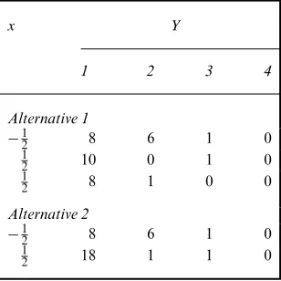
For example, consider the two representations of the same data in Table 3. Interest is in estimating the differenceβ between logits of cumulative probabilities of the samples withx= −12 from the samples withx=21.
The maximum likelihood estimate ofα3is∞. Irrespective of the data representation the
maximum likelihood estimate ofβis finite and has value−1.944 with estimated standard error 0.895. Now suppose that the same small constant, say 12, is added to each of the counts in the rows of the alternatives in Table 3. The adjustment ensures that the parame-ter estimates are finite for both representations. Nevertheless, a common constant added to both alternatives causes—in some cases large—differences in the resultant inferences forβ. For alternative 1 the maximum likelihood estimate ofβbased on the adjusted data is−1.097 with estimated standard error 0.678, and for alternative 2 the estimate is−1.485 with estimated standard error 0.741. If Wald-type procedures were used for inferences on βwith a normal approximation for the distribution of the approximate pivot.βˆ−β/=S.βˆ/, whereS.β/is the asymptotic standard error atβbased on the Fisher information, then the p-value of the testβ=0 would be 0.106 if alternative 1 was used and 0.045 if alternative 2 was used.
[image:11.612.164.318.567.721.2](b) Furthermore, the moments of the maximum likelihood estimator generally depend on the parameter values (see, for example, Cordeiro and McCullagh (1991) for explicit expres-sions of the first-order bias term in the special case of binomial regression models) and
Table 3. Two alternative representations of the same artificial data set
x Y
1 2 3 4
Alternative 1
−1
2 8 6 1 0
1
2 10 0 1 0
1
2 8 1 0 0
Alternative 2
−1
2 8 6 1 0
1
thus, as is also amply evident from the studies in Hitchcock (1962) and Gartet al.(1985), there cannot be a universal constant which yields estimates which are optimal according to some frequentist criterion.
Both of the above concerns with constant adjustment schemes are dealt with by using the additive adjustment scheme in Section 5.1. Firstly, by construction, the iteration of Section 5.1 yields estimates which have bias of second order. Secondly, because the adjustments depend on the parameters only through the linear predictors which, in turn, do not depend on the way that the data are represented, the adjustment scheme leads to estimators that are invariant to the data representation. For both representations of the data in Table 3 the bias-reduced estimate ofβis−1.761 with estimated standard error 0.850.
7. Invariance properties of the reduced bias estimator
7.1. Equivariance under linear transformations
The maximum likelihood estimator is exactly equivariant under one-to-one transformations φ.·/of the parameterδ, i.e. if ˆδis the maximum likelihood estimator ofδthen the maximum likelihood estimator of φ.δ/ is simplyφ.δ/ˆ . In contrast with ˆδ, the reduced bias estimator
˜
δRB is not equivariant for all φ; bias is a parameterization-specific quantity and hence any
attempt to improve it can violate exact equivariance. Nevertheless,δ˜RB is equivariant under
linear transformationsφ.δ/=Lδ, whereLis a.p+q/×.p+q/matrix of constants such that ZLis of full rank andδ=Lδhasα1<: : :<αq.
To see that, assume that we fit the multinomial model withγrs=G.ηrs/whereηrs =Σpt=+1qδtzrst .r=1,: : :,n;s=1,: : :,q/. Becauseδ=Lδ,ηrs is a linear combination ofδ. Using expression (9), thetth component of the adjusted score function forδis
U t=
n
r=1
q
s=1
g rs
yrs+crs−crs−1
πrs −
yrs+1+crs+1−crs
π rs+1
zrst, .13/
fort∈{1,: : :,p+q}, wherecrs ,πrs andgrsare evaluated atδ. Note that all quantities in equation (13) depend onδonly through the linear combinationsηrs . Thus, comparing equation (9) with equation (13), ifδ˜RBis a solution ofUÅt =0.t=1,: : :,p+q/, thenLδ˜RBmust be a solution of U
t=0.t=1,: : :,p+q/.
The bias-corrected estimator defined in equation (10) can be shown also to be equivariant under linear transformations, using the equivariance of the maximum likelihood estimator and the fact thatb.δ/depends onδonly through the linear predictors.
7.2. Invariance under reversal of the order of categories
One of the properties of proportional odds models, and generally of cumulative link models with a symmetric latent distribution G.·/, is their invariance under the reversal of the order of categories; a reversal of the categories along with a simultaneous change of the sign ofβ and change of sign—and hence order—toα1,: : :,αqin model (2) results in the same category
probabilities. Given the usual arbitrariness in the definition of ordinal scales in applications this is a desirable invariance property for the analysis of ordinal data.
The maximum likelihood estimator respects this invariance property, i.e. if the categories are reversed then the new fit can be obtained by merely using−βˆMLfor the regression parameters and.−αˆq,: : :,−αˆ1/for the cut points.
180 I. Kosmidis
with α1<: : : <αq. Because g.·/ is symmetric about zero, G.η/=1−G.−η/, and so γrs= G.−αk−s+βTx
r/. This is a reparameterization of model (3) to γrs=G.Σpt=+1qδtzrst/ where
δ=.α
1,: : :,αq,β1,: : :,βp/T=.−αq,: : :,−α1,−β1,: : :,−βp/T. Hence,δ=Lδwith
L=
⎛ ⎜ ⎜ ⎜ ⎜ ⎝
0 : : : 0 −1 0
0 : : : −1 0 0
::: ::: ::: ::: :::
−1 : : : 0 0 0
0 : : : 0 0 −1
⎞ ⎟ ⎟ ⎟ ⎟ ⎠,
and, using the results of Section 7.1,δ˜RB=Lδ˜RB(and alsoδ˜BC=Lδ˜BC).
8. Properties of the reduced bias estimator and associated inferential procedures: a complete-enumeration study
8.1. Study design
The frequentist properties of the reduced bias estimator are investigated through a complete-enumeration study of 2×k contingency tables with fixed row totals. The rows of the tables correspond to a two-level covariatexwith valuesx1andx2, and the columns to the levels of
an ordinal responseY with categories 1,: : :,k. The row totals are fixed tom1for x=x1and
tom2forx=x2. Alternative 2 in Table 3 is a special case withk=4,x1= −12,x2=12, and row
totalsm1=15 andm2=20. The present complete enumeration involves.m1m1+q/.m2m2+q/tables.
We consider a multinomial model with
γ1s=G.αs−βx1/, γ2s=G.αs−βx2/ .s=1,: : :,q/, .14/
whereα1,: : :,αqare regarded as nuisance parameters but are essential to be estimated from the
data, because they allow flexibility in the probability configurations within each of the rows of the table.
For the estimation ofβwe consider the maximum likelihood estimator ˆβ, the bias-corrected estimatorβ˜BC, the reduced bias estimatorβ˜RBand the generalized empirical logistic transform ˆ
βEL which is defined in McCullagh (1980), section 2.3, and is an alternative estimator with smaller asymptotic bias than the maximum likelihood estimator specifically engineered for the estimation ofβ in 2×ktables with fixed row totals. The estimators ˆβ,β˜BCandβ˜RBare theβ -components of the vectors of estimators ˆδ,δ˜BCandδ˜RBrespectively, whereδ=.α1,: : :,αq,β/T
is the vector of all parameters. The estimators are compared in terms of bias, mean-squared error and coverage probability of the respective Wald-type asymptotic confidence intervals. The following theorem is specific to 2×kand cumulative link models and can be used to reduce the parameter settings that need to be considered in the current study for evaluating the performance of the estimators.
Theorem 1. Consider a 2×kcontingency tableT with fixed row totalsm1andm2, and the
multinomial model that satisfies expression (14). Furthermore, consider an estimatorδÅ.T/ ofδ, which is equivariant under linear transformations. Then, ifm1=m2, the bias function
and the mean-squared error ofβÅ.T/satisfy
E{βÅ.T/−β;β,α}= −E{βÅ.T/+β;−β,α}
E[{βÅ.T/−β}2;β,α]=E[{βÅ.T/+β}2;−β,α] respectively.
Proof. Define an operatorRwhich when applied toT results in a new contingency table by reversing the order of the rows ofT. Hence,R{R.T/}=T.
BecauseδÅ.T/is equivariant under linear transformations, it suffices to study the behaviour ofβÅ.T/whenx1= −12 andx2=12. Then, any combination of values forx1andx2results by
an affine transformation of the vector .−12,12/, and equivariance gives that a corresponding translation of the vectorαÅ.T/and change of scaling ofβÅ.T/results in exactly the same fit. Hence, the shape properties ofβÅ.T/remain invariant to the choice of.x1,x2/T.
Denote withT the set of all possible 2×ktables with fixed row totalsm1andm2. By the
definition of the model,P.T;β,α/=P{R.T/;−β,α}for everyT∈T. Becausem1=m2 there
is a subset E⊂T of tables with .y11,: : :,y1k/=.y21,: : :,y2k/. The complement of E can be partitioned into the setsF1andF2which have the same cardinality, and whereT∈F1if and only
ifR.T/∈F2. Forx1= −12andx2=12, equivariance under the linear transformationφ.β/= −β
gives thatβÅ.T/= −βÅ{R.T/}. Then, for anyT∈E,βÅ.T/=0. Hence, E{βÅ.T/;β,α}=
T∈EβÅ.T/P.T;β,α/ .15/
=
T∈E,T∈F1
βÅ.T/[P.T;β,α/−P{R.T/;β,α}]
=
T∈E,T∈F1
βÅ.T/[P{R.T/;−β,α}−P.T;−β,α/]
= −E{βÅ.T/;−β,α}:
Adding−β to both sides of this equality gives the identity on the bias. For the identity on the mean-squared error one merely needs to repeat a corresponding calculation to equation (15) starting from
E[{βÅ.T/−β}2;β,α]=
T∈E{βÅ.T/−β}
2P.T;β,α/+β2
T∈EP.T;β,α/:
A similar line of proof can be used to show that ifm1=m2the coverage probability of
Wald-type asymptotic confidence intervals forβis symmetric aboutβ=0, provided that the estimator S.T/of the standard error ofβÅ.T/satisfiesS.T/=S{R.T/}.
8.2. Special case: proportional odds model
For demonstration purposes, the values of the competing estimators are obtained for a propor-tional odds model (G.η/=exp.η/={1+exp.η/}) withx1= −12 andx2=12 andk=4, for each
of the 400, 3136 and 81796 possible tables with row totalsm=m1=m2, form=3,m=5 and m=10 respectively. All estimators considered are equivariant under linear transformations and hence, according to the proof of theorem 1, the outcome of the complete enumeration for the comparative performance of the estimators generalizes to any choice of.x1,x2/T.
182 I. Kosmidis
For evaluating the performance of the estimators, the probability of each of the tables has been calculated under model (14), for parameter values that are fixed according to the following scheme. The parameterβtakes values on some sufficiently fine equispaced grid in the interval [−6, 0]. Forβ in the interval.0, 6] the results can be predicted by the symmetry relations of theorem 1. For each value ofβ, the nuisance parameters take values.α1,α2,α3/T=e.−1, 0, 1/T
fore∈{1, 2, 3, 5, 7}. Fig. 1 is a pictorial representation of the probability settings for the two multinomial vectors in the 2×4 contingency table with fixed row totals, at each combination of values for β and .α1,α2,α3/T. (The left-hand side of each plot depicts the multinomial
probabilities forx= −12 and the right-hand side the multinomial probabilities forx=12. The eight probabilities (four for eachx-value) for each particular combination of values forβand .α1,α2,α3/are connected with line segments. Hence each piecewise linear function on each plot
corresponds to a specific probability setting for the 2×4 contingency table with fixed row totals. The plots correspond to particular settings for the nuisance parameters.α1,α2,α3/determined
bye.−1, 0, 1/, and each plot contains all possible piecewise linear functions for the values of β on an equispaced grid of size 50 in the interval [−6, 6].) Under the above scheme for fixing parameter values, the probability of the end categories tends to 0 aseincreases, and hence more extreme probability settings are being considered asegrows.
The findings of the current complete-enumeration exercise are outlined in the following subsection. The same complete-enumeration design has been applied to various settings, with m1=m2, with different link functions, with different numbers of categories and/or for
differ-ent non-symmetric specifications for the nuisance parameters (the results are not shown here) yielding qualitatively the same conclusions; the current set-up merely allows a clear pictorial representation of the findings on the behaviour of the reduced bias estimator. An R script that can produce the results of the current complete enumeration for any number of categories, any link function, any configuration of totals and any combination of parameter settings in 2×k contingency tables is available in the on-line supplementary material.
8.3. Remarks on the results
Remark 1(on the estimates ofα1,α2andα3). According to Section 3, for data sets where a
specific categorys∈{1, 2, 3, 4}is observed for neitherx=−12norx=12, the maximum likelihood estimate ofαis on the boundary of the parameter space as follows:
s=1, αˆ1= −∞; s=2, αˆ2=αˆ1; s=3, αˆ3=αˆ2; s=4, αˆ3= ∞:
At least for log-concaveg.·/, according to the results in Pratt (1981), these equations extend directly to the case of any number of categories and number of covariate settings and can directly be used to check what happens when two or more categories are unobserved.
Nevertheless, the maximum likelihood estimator ofβis invariant to merging a non-observed category with either the previous or next category and can be finite even if some of the α -parameters are on the boundary of the parameter space. Hence, maximum likelihood inferences onβ are possible even if a category is not observed. The same behaviour is observed for the reduced bias estimators ofα1,α2andα3with the difference that, if the non-observed category
iss=1 and/ors=4, thenα˜1,RBand/orα˜3,RBare finite. A special case of this observation has
184 I. Kosmidis
end categories, guaranteeing the finiteness of the cumulative logits. Hence, there is no need for non-observed end categories to be merged with the neighbouring categories when the reduced bias estimator is used. If any of the other categories is empty, then the reduced bias estimator ofβis invariant to merging those with any of the neighbouring categories.
It should be mentioned here that if both the second and the third category are empty then the reduced bias estimate ofβand the generalized empirical logistic transform are identical. To see that, note that, in the special case of logistic regression, the adjusted scores in Section 4.4 suggest adding half a leverage to each ofyr1andyr2.r=1, 2/(this result for logistic regressions
was obtained in Firth (1993)). Furthermore, the model withq=1 is saturated and hence both leverages are 1. Hence the reduced bias estimate ofβcoincides with the generalized empirical logistic transform, which fork=2 is log{.y11+12/=.m1−y11+21/}−log{.y21+12/=.m2−y21+
1
2/}.
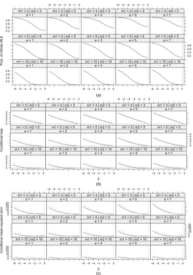
Remark 2(on ˆβ andβ˜BC). As is expected from the discussion in Section 3, the maximum likelihood estimator ofβ is infinite for certain configurations of 0s in the table, and for such configurations the bias-corrected estimator is also undefined owing to its explicit dependence on the maximum likelihood estimator. Hence, for ˆβandβ˜BC, the bias function is undefined and the mean-squared error is infinite. A possible comparison of the performance of ˆβandβ˜BCis in terms of conditional bias and conditional mean-squared error where the conditioning event is that ˆβhas a finite value.
For detecting parameters with infinite values the diagnostics in Lesaffre and Albert (1989), section 4, for multinomial logistic regressions are adapted to the current setting. Data sets that result in infinite estimates forβhave been detected by observation of the size of the corresponding estimated standard error based on the inverse of the Fisher information, and by observation of the absolute value of the estimates when the convergence criteria were satisfied. If the standard error was greater than 200 and the estimate was greater than 100, then the estimate was labelled infinite. A second pass through the data sets has been performed, making the convergence criterion for the Fisher scoring stricter than|Ut.δc/|<10−10. The estimates that were labelled
infinite by using the aforementioned diagnostics further diverged towards∞whereas the rest of the estimates remained unchanged to high accuracy.
The probability of encountering an infinite ˆβ for the different possible parameter settings is shown in Fig. 2(a). Forβ∈.0, 6/the probability of encountering an infinite value is simply a reflection of the probability in.−6, 0/acrossβ=0. As is apparent the probability of infinite estimates increases aseincreases and for each value ofeit increases as|β|increases. As is natural asmincreases, the probability of encountering infinite estimates is reduced but is always posi-tive.
Of course, the findings from the current comparison of ˆβ withβ˜BC should be interpreted critically, bearing in mind the conditioning on the finiteness of ˆβ; the comparison suffers from the fact that the first-order bias term that is required for the calculation ofβ˜BCis calculated unconditionally. The comparison is fairer when the probability of infinite estimates is small; this happens on a region around zero whose size also increases asmincreases.
The conditional bias and conditional mean-squared error of ˆβandβ˜BCare shown respectively in Fig. 2(b) and Fig. 2(c). The identities in theorem 1 apply also to the conditional and conditional mean-squared error; to see this setPto be the conditional probability of each table in the proof of theorem 1. Hence, forβ∈.0, 6/, the conditional bias is simply a reflection of the conditional bias forβ∈.−6, 0/across the 45◦line, and the conditional mean-squared error is a reflection of the conditional mean-squared error forβ∈.−6, 0/acrossβ=0.
β Conditional bias 0 1 2 3 4 5
−6 −5 −4 −3 −2 −1 0
e = 1 m1 = 10 | m2 = 10
e = 2 m1 = 10 | m2 = 10
−6 −5 −4 −3 −2 −1 0
e = 3 m1 = 10 | m2 = 10
e = 5 m1 = 10 | m2 = 10
−6 −5 −4 −3 −2 −1 0
e = 7 m1 = 10 | m2 = 10 e = 1
m1 = 5 | m2 = 5
e = 2 m1 = 5 | m2 = 5
e = 3 m1 = 5 | m2 = 5
e = 5 m1 = 5 | m2 = 5
0 1 2 3 4 5 e = 7
m1 = 5 | m2 = 5 0 1 2 3 4 5
e = 1 m1 = 3 | m2 = 3
−6 −5 −4 −3 −2 −1 0
e = 2 m1 = 3 | m2 = 3
e = 3 m1 = 3 | m2 = 3
−6 −5 −4 −3 −2 −1 0
e = 5 m1 = 3 | m2 = 3
e = 7 m1 = 3 | m2 = 3
Prob. of infinite MLE
0.2 0.4 0.6 0.8
−6 −5 −4 −3 −2 −1 0
e = 1 m1 = 10 | m2 = 10
e = 2 m1 = 10 | m2 = 10
−6 −5 −4 −3 −2 −1 0
e = 3 m1 = 10 | m2 = 10
e = 5 m1 = 10 | m2 = 10
−6 −5 −4 −3 −2 −1 0
e = 7 m1 = 10 | m2 = 10 e = 1
m1 = 5 | m2 = 5
e = 2 m1 = 5 | m2 = 5
e = 3 m1 = 5 | m2 = 5
e = 5 m1 = 5 | m2 = 5
0.2 0.4 0.6 0.8 e = 7
m1 = 5 | m2 = 5 0.2
0.4 0.6 0.8
e = 1 m1 = 3 | m2 = 3
−6 −5 −4 −3 −2 −1 0
e = 2 m1 = 3 | m2 = 3
e = 3 m1 = 3 | m2 = 3
−6 −5 −4 −3 −2 −1 0
e = 5 m1 = 3 | m2 = 3
e = 7 m1 = 3 | m2 = 3
β
Conditional mean-squared error
0 5 10 15 20 25
−6 −5 −4 −3 −2 −1 0
e = 1 m1 = 10 | m2 = 10
e = 2 m1 = 10 | m2 = 10
−6 −5 −4 −3 −2 −1 0
e = 3 m1 = 10 | m2 = 10
e = 5 m1 = 10 | m2 = 10
−6 −5 −4 −3 −2 −1 0
e = 7 m1 = 10 | m2 = 10 e = 1
m1 = 5 | m2 = 5
e = 2 m1 = 5 | m2 = 5
e = 3 m1 = 5 | m2 = 5
e = 5 m1 = 5 | m2 = 5
0 5 10 15 20 25 e = 7
m1 = 5 | m2 = 5 0 5 10 15 20 25
e = 1 m1 = 3 | m2 = 3
−6 −5 −4 −3 −2 −1 0
e = 2 m1 = 3 | m2 = 3
e = 3 m1 = 3 | m2 = 3
−6 −5 −4 −3 −2 −1 0
e = 5 m1 = 3 | m2 = 3
e = 7 m1 = 3 | m2 = 3
(a)
(b)
[image:18.612.58.437.145.684.2](c)
186 I. Kosmidis
likelihood estimator performing slightly better thanβ˜BCfor smallm. Asmincreases the bias-corrected estimator starts to perform better in terms of bias in a region around zero, where the probability of infinite estimates is smallest. The same is noted for the conditional mean-squared error. The estimatorβ˜BCperforms better than ˆβin a region around zero, whose size increases asmincreases. The same behaviour as fore=7 persists for larger values ofe(the figures are not shown here).
Remark 3(on ˆβELandβ˜RB). The estimators ˆβELandβ˜RBalways have finite value irrespective of the configuration of 0s in the table. Hence, in contrast with ˆβ andβ˜BC, a comparison in terms of their unconditional bias and unconditional mean-squared error is possible. Fig. 3(a) shows the bias function of the estimator for the parameter settings that were considered in the complete-enumeration study. Forβ∈.0, 6/, the bias function is simply a reflection of the bias for β∈.−6, 0/across the 45◦line, and the mean-squared error is a reflection of the mean-squared error forβ∈.−6, 0/acrossβ=0.
β Bias 0 1 2 3
−6 −5 −4 −3 −2 −1 0
e = 1 m1 = 10 | m2 = 10
e = 2 m1 = 10 | m2 = 10
−6 −5 −4 −3 −2 −1 0
e = 3 m1 = 10 | m2 = 10
e = 5 m1 = 10 | m2 = 10
−6 −5 −4 −3 −2 −1 0
e = 7 m1 = 10 | m2 = 10 e = 1
m1 = 5 | m2 = 5
e = 2 m1 = 5 | m2 = 5
e = 3 m1 = 5 | m2 = 5
e = 5 m1 = 5 | m2 = 5
0 1 2 3 e = 7
m1 = 5 | m2 = 5 0
1 2 3
e = 1 m1 = 3 | m2 = 3
−6 −5 −4 −3 −2 −1 0
e = 2 m1 = 3 | m2 = 3
e = 3 m1 = 3 | m2 = 3
−6 −5 −4 −3 −2 −1 0
e = 5 m1 = 3 | m2 = 3
e = 7 m1 = 3 | m2 = 3
β Mean-squared error 2 4 6 8 10
−6 −5 −4 −3 −2 −1 0
e = 1 m1 = 10 | m2 = 10
e = 2 m1 = 10 | m2 = 10
−6 −5 −4 −3 −2 −1 0
e = 3 m1 = 10 | m2 = 10
e = 5 m1 = 10 | m2 = 10
−6 −5 −4 −3 −2 −1 0
e = 7 m1 = 10 | m2 = 10 e = 1
m1 = 5 | m2 = 5
e = 2 m1 = 5 | m2 = 5
e = 3 m1 = 5 | m2 = 5
e = 5 m1 = 5 | m2 = 5
2 4 6 8 10 e = 7
m1 = 5 | m2 = 5 2
4 6 8 10
e = 1 m1 = 3 | m2 = 3
−6 −5 −4 −3 −2 −1 0
e = 2 m1 = 3 | m2 = 3
e = 3 m1 = 3 | m2 = 3
−6 −5 −4 −3 −2 −1 0
e = 5 m1 = 3 | m2 = 3
[image:19.612.46.438.332.715.2]e = 7 m1 = 3 | m2 = 3
The reduced bias estimator performs better than ˆβEL in terms of bias for small values ofe and the differences in the bias functions diminish aseincreases. A similar limiting behaviour holds for their mean-squared errors, though, for small values ofe, ˆβELperforms slightly better thanβ˜BRin terms of mean-squared error in the range.−4, 4/and worse outside that range. The mean-squared error of both estimators converges to 0 asmincreases, which is what is expected from consistent estimators (see Kosmidis (2007a), section 6.3, for a proof of the consistency of the reduced bias estimator).
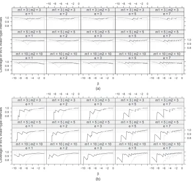
Remark 4(on the coverage of 95% Wald confidence intervals). For a tableTand an estimator βÅ.T/, consider the nominally 100.1−a/% Wald-type confidence interval forβ
βÅ.T/±z1−a=2SÅ.T/,
wherezais the 100ath quantile of a standard normal distribution andSÅ.T/is the estimator of the standard error ofβÅ.T/. For ˆβ,β˜BCandβ˜RB,SÅ.T/is taken to be the square root of the diagonal element of the inverse of the Fisher information corresponding toβ, evaluated at ˆβ.T/, β˜BC.T/ and β˜RB.T/ respectively. For the estimation of the standard error for ˆβEL, the variance formula that was given in McCullagh (1980), section 2.3, is used. If the maximum likelihood estimate is infinite then we make the convention that the confidence intervals based on
ˆ
βandβ˜BCare.−∞,∞/. Fig. 4 shows the coverage probabilities of the four competing intervals for α=e.−1, 0, 1/T withe∈{1, 2, 3, 5, 7}, and for β∈[−10, 0]. The coverage probability for
β∈.0, 10/is simply a reflection of the coverage probability forβ∈.−10, 0/acrossβ=0. Wald-type confidence intervals based on the maximum likelihood estimator demonstrate a conservative behaviour in terms of coverage, and the coverage probability converges to 1 as |β|→∞. Furthermore, the coverage probability seems to approach uniformly the nominal level asmincreases. The intervals based on the bias-corrected estimator also demonstrate conservative behaviour in a neighbourhood aroundβ=0, then tend to undercover for an interval of large |β|-values and, as for ˆβ, when|β| → ∞the coverage probability tends to 1.
A more dramatic undercoverage is present for confidence intervals that are based on ˆβEL when|β|is large. Actually after some value of|β|the confidence intervals that are based on
ˆ
βEL completely lose coverage (the full range of the coverage probability is not shown here). In contrast, those intervals behave satisfactorily around β=0. This behaviour relates to the fact that the variance estimator for ˆβELis obtained under the assumption thatβ=0 and can seriously underestimate the variance of ˆβELwhen |β|is larger than about 1 (the same obser-vation was also made in McCullagh (1980), section 2.3). Furthermore, it is worth noting that the point where coverage is lost completely moves closer to zero asmincreases. Hence, use of Wald-type confidence intervals that are based on ˆβEL is not recommended in practical applications.
188 I. Kosmidis
β Coverage of 95% Wald−type intervals 0.8
0.9 1.0
−10 −8 −6 −4 −2 0 e = 1 m1 = 10 | m2 = 10
e = 2 m1 = 10 | m2 = 10
−10 −8 −6 −4 −2 0 e = 3 m1 = 10 | m2 = 10
e = 5 m1 = 10 | m2 = 10
−10 −8 −6 −4 −2 0 e = 7 m1 = 10 | m2 = 10 e = 1
m1 = 5 | m2 = 5
e = 2 m1 = 5 | m2 = 5
e = 3 m1 = 5 | m2 = 5
e = 5 m1 = 5 | m2 = 5
0.8 0.9 1.0 e = 7
m1 = 5 | m2 = 5 0.8
0.9 1.0
e = 1 m1 = 3 | m2 = 3
−10 −8 −6 −4 −2 0
e = 2 m1 = 3 | m2 = 3
e = 3 m1 = 3 | m2 = 3
−10 −8 −6 −4 −2 0
e = 5 m1 = 3 | m2 = 3
e = 7 m1 = 3 | m2 = 3
(a)
[image:21.612.45.441.148.519.2](b)
Fig. 4. Coverage probabilities of nominally 95% asymptotic Wald-type confidence intervals forβbased on (a) ˆβ( ) and ˜βBC( ) and (b) ˆβEL( ) and ˜βRB( ) and the respective standard errors, forβ2[10, 0/andαDe.1, 0, 1/Tfore2{1, 2, 3, 5, 7}
of the necessarily discrete distribution of the reduced bias estimator by a normal distribution with variance the inverse of the Fisher information becomes more accurate. This results in the increasing accuracy of the approximation of the distribution of the Wald pivot by a normal distribution.
9. Shrinkage towards a binomial model for the end categories
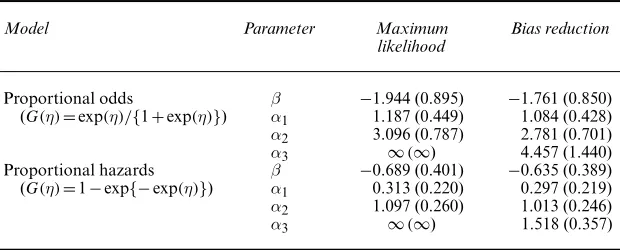
Table 4 shows the maximum likelihood estimates, the reduced bias estimates and the corres-ponding estimated standard errors from fitting a proportional odds model and a proportional hazards model of the form (14) to the artificial data that were considered in the example in Section 6.2.
There is apparent shrinkage of the reduced bias estimates towards 0, which implies a shrinkage of the cumulative probabilities towardsG.0/. This implies a shrinkage of the probabilities for the first and the last category of the ordinal scale towardsG.0/and 1−G.0/respectively, and a corresponding shrinkage of the probabilities of the intermediate categories towards 0.
To investigate further the apparent shrinkage effect, the maximum likelihood and reduced bias estimates of proportional odds and proportional hazards models of the form (14) are obtained for every possible 2×6 table with row totalsm1=m2=3. This setting is chosen because it is
one that results in sparse tables, allowing the construction of plots of fitted probabilities that are not massively overcrowded (under this setting there are 3136 tables to be estimated).
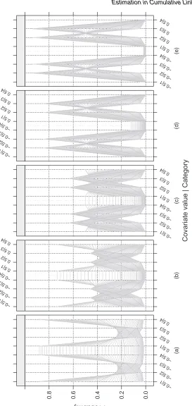
For each category of the ordinal response, Fig. 5 shows the fitted probabilities based on the reduced bias estimator against the fitted probabilities based on the maximum likelihood estimator. The grey areas are where the points would all be expected to lie if the shrinkage relationships were strictly satisfied for each pair of fitted probabilities. Clearly this is not so.
The points on the plots for the first category roughly lie slightly above the 45◦line for fitted values less thanG.0/, and slightly below it for fitted values greater thanG.0/. The points for the last category exhibit similar behaviour but withG.0/replaced by 1−G.0/. The shrinkage effect appears to be stronger the further the probability is from the shrinkage pointsG.0/and 1−G.0/.
The points on the plots for the intermediate categories lie mostly under the 45◦line, except in cases where the maximum-likelihood-fitted probability is very close to 0. Hence, the fitted probabilities for the intermediate categories based on the reduced bias estimator tend to shrink towards 0. The plots also suggest that the further the probability is from 0 the stronger is the shrinkage effect.
[image:22.612.92.402.596.721.2]The shrinkage properties that are observed here are a direct generalization of the shrinkage that is implied by improving bias in the estimation of binomial logistic regression models (Copas, 1988; Cordeiro and McCullagh, 1991; Firth, 1992) to links other than the logistic and to models with ordinal responses.
Table 4. Parameter estimates and corresponding estimated standard errors (in paren-theses) from fitting a proportional odds model and a proportional hazards model of the form (14) to the artificial data considered in Table 3 in Section 6.2, using maximum likelihood and bias reduction
Model Parameter Maximum Bias reduction
likelihood
Proportional odds β −1.944 (0.895) −1.761 (0.850)
(G.η/=exp.η/={1+exp.η/}) α1 1.187 (0.449) 1.084 (0.428)
α2 3.096 (0.787) 2.781 (0.701)
α3 ∞.∞) 4.457 (1.440)
Proportional hazards β −0.689 (0.401) −0.635 (0.389)
(G.η/=1−exp{−exp.η/}) α1 0.313 (0.220) 0.297 (0.219)
α2 1.097 (0.260) 1.013 (0.246)
Corresponding empirical investigations of shrinkage based on both complete enumerations and simulations under models fitted to real data have also been performed but are not shown here. The results are qualitatively the same: reduction of bias in cumulative link models shrinks the multinomial model towards a binomial model that has probabilityG.0/for the first category and probability 1−G.0/for the last category.
10. Simulation study
To illustrate further the properties of the reduced bias estimator in more complex scenarios than that in the complete-enumeration study of Section 8, a simulation study was set up based on part of the data that have been analysed in Jackman (2004). The data are publicly available through the R packagepscl(Jackman, 2012) and seem to agree with the data that are available for rater F1 in the analysis in Jackman (2004). The data contain the score of rater F1 for 106 applications to the political science doctoral programme at Stanford University along with corresponding applicant-specific observations. The rater’s score is on a five-point integer-valued ordinal scale from 1 to 5, with 1 indicating the lowest rating and 5 indicating the highest rating. Consider that the cumulative log-odds for ratingsfor therth candidate is modelled as
log
γ
rs 1−γrs
=αs−β1xr1−β2xr2−β3zr1−β4zr2−β5gr .r=1,: : :, 106;s=1,: : :, 4/, .16/ wherexr1andxr2are therth applicant’s scores on the quantitative and verbal section of the
grad-uate record examinations respectively (after subtracting the respective mean and dividing by the respective standard deviation),zr1andzr2are dummy variables indicating whether therth
ap-plicant has an interest in American politics and political theory respectively (with 1 representing a positive and 0 a negative reply), andgris the gender of therth applicant.r=1,: : :, 106/. The parametersα1,: : :,α5are the cut points andβ1,: : :,β5describe the effect of the corresponding
applicant-specific covariates on the cumulative log-odds.
Model (16) was fitted by using maximum likelihood and the maximum likelihood estimates ofβ1,: : :,β5are 1.993, 0.892, 2.816, 0.009 and 1.215 respectively, indicating that an increase in
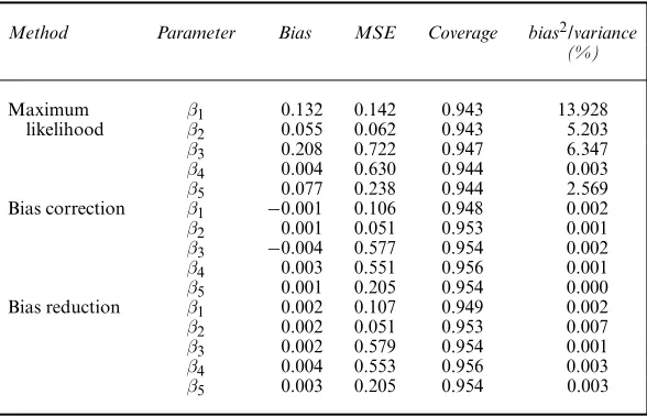
the value of any of the covariates is associated with higher probability for high ratings holding all else in the model fixed. Then an extensive simulation under the maximum likelihood fit is performed for estimating the biases, mean-squared errors and coverage probabilities of Wald-type 95% confidence intervals forβ1,: : :,β5 when maximum likelihood, bias correction and
bias reduction are used. There have been instances of simulated data sets where one or more rating categories were empty. In those cases, empty categories were merged with neighbouring categories according to the discussion in remark 1 of Section 8. The results are shown in Table 5. There was only one data set for which the maximum likelihood estimate ofβ3was∞. This data
set was excluded when estimating the bias, mean-squared error and coverage probability for the maximum likelihood and the bias-corrected estimator and hence the corresponding figures in Table 5 estimate the conditional respective quantities (i.e. given that the maximum likelihood estimator has finite value). In contrast, the reduced bias estimates were finite for all data sets and hence the corresponding figures are estimates of the targeted unconditional quantities. In this particular setting, the probability of the conditioning event is small and a direct comparison of the estimated conditional and unconditional quantities can be informative.