Designing a Machine Learning Decision Tree for Information Systems: A study into the implementation of supervised and unsupervised machine learning methods

(1)

Designing a Machine Learning Decision Tree

for Information Systems:

A study into the implementation of supervised and

unsupervised machine learning methods

Bas van Tintelen

BSC Industrial Engineering and Management

s1866494

(2)

Graduate

Bas van Tintelen

s1866494

BSc Industrial Engineering and Management

CAPE Groep BV

CAPE Groep BV Supervisor

Transportcentrum 14

Mr. B. Knol

7547 RW Enschede

Manager Customer Support

Netherlands

CAPE Groep

www.capegroep.nl

University of Twente

Drienerlolaan 5

7522 NB Enschede

Netherlands

www.utwente.nl

University of Twente First Supervisor

University of Twente Second Supervisor

Dr. N. Knofius

Dr. L. O. Meertens

Postdoc

Assistant Professor

Dep. of Industrial Engineering and

Business Information Systems

(3)

Preface

Dear Reader,

This report indicates the end of my Bachelor Thesis Assignment for my bachelor Industrial

Engineering Management study at the University of Twente conducted on behalf of CAPE

Groep’s support department. My Bachelor Thesis has been a challenging, time-consuming,

brain-teasing, but above all an interesting and informative experience. During my Bachelor

Thesis Assignment, I explored the possibilities of machine learning in CAPE Groep’s

information systems. This report contains the research I conducted, starting with

preparation and concluding with the results and recommendations to the company.

I would like to start by giving credits where they are due. First of all, I want to thank CAPE

Groep, in particular, the support department, for helping me conducting this research and

aiding me whenever I needed assistance. I especially want to thank Bart Knol, head of the

support department, for guiding me through the weeks and providing the necessary

information needed for this research. Also, I want to thank Gilang Charismadiptya, support

department employee, for guiding me through the different websites and applications to

gain insight into CAPE Groep’s information systems.

Furthermore, I want to thank my supervisors from the University of Twente, Nils Knofius

and Lucas Meertens. Nils assisted me with his machine learning knowledge and provided

essential feedback on the structure of the report. Lucas increased the academic level of the

report by aiding with defining the design artefact and tweaking the writing style of the

report.

I want to end with thanking Kaleb Dan, Wim Klaassen, Ruben Lucas, Thijmen Meijer,

Alexander Stekelenburg, Mariëlle van Tintelen, Frits Tuininga and Armando van Vlastuin

who helped me carry on, provided feedback and gave advice to improve my research.

I hope you will find this report an educational and pleasant read.

(4)

Management Summary

A decision tree for predicting and detecting software breakdowns using machine learning

techniques has been created during this research. It provides guidance for implementing

suitable machine learning algorithms in information systems. The created decision tree is

focused on both the supervised classification and unsupervised anomaly detection

algorithms. By going through the decision tree some data shortcomings might be found.

Several options to tackle these shortcomings are provided during an elaboration of the

decision tree. When the decision tree is followed the practitioner has gained an overview of

machine learning requirements that are not yet fulfilled as well as several methods to fulfil

the unmet requirements. The application of the decision tree is demonstrated based on the

situation of the company’s support department.

The researched machine learning types, supervised classification and unsupervised anomaly

detection, can both be used to, respectively, predict and detect breakdowns of software.

Both types need different input and therefore provide different possibilities. Supervised

classification needs data that contains a label for each feature set whether or not an error

occurred. This data is then used to predict whether or not an error can be expected for a

new feature set. The downside of this method is that labelling the data often turns out to be

a time-consuming and costly endeavour. Unsupervised anomaly detection does not need

labelled data but needs data with a lot of normal behaving feature sets. The algorithms use

this data to detect abnormal behaviour in new feature sets which might cause errors. The

drawback is that normal behaving data and error data are sometimes hard to distinguish.

CAPE Groep’s support department has to monitor and maintain a growing number of

Mendix and eMagiz applications. As this makes up a large portion of their day-to-day tasks,

they want to know beforehand if and when their applications might breakdown, so they can

preemptively maintain their applications and provide a higher uptime to their clients. They

are changing their data saving architecture as well as their monitoring dashboard to get a

better insight into the health status of the applications. They want to start with

implementing types of artificial intelligence that will help them maintain and monitor their

applications. However, the stored Mendix application data does not yet fulfil the

requirements of either machine learning type.

The application of the decision tree on the support department’s current situation yielded

that the support department should focus on unsupervised anomaly detection. This is the

preferred machine learning type due to the lack of breakdown data, which makes it

impossible to train the supervised classification algorithms. In order to start using

(7)

6

Reader’s guide

In this part, I will address the structure of the report as well as the abbreviations and definitions I used.

Report Structure.

My report contains six chapters and three appendices.

Chapter 1 | Context Analysis In this chapter I describe both the company and the support department on which behalf this research is conducted. I will continue by defining the action problem and the steps I took to get to the core problem of this research. After identifying the core problem I will address the research objective and measurement of the solution. Then I address the motivation behind solving this core problem. I will conclude this chapter with a list of knowledge questions that I had to answer and discuss the used research methodology.

Chapter 2 | Literature Review During this chapter I will elaborate on the literature reviews I

conducted for the needed machine learning knowledge. I will start the chapter with an introduction of machine learning and its types. The next two sections of this chapter are devoted to supervised classification and unsupervised anomaly detection and their most applicable algorithms. I will conclude this chapter with a description of how to test and compare the different algorithms to find the most applicable algorithm for a similar data set.

Chapter 3 | Solution Design In this chapter I will explain the created design artefact, a decision tree with branches for both supervised classification and unsupervised anomaly detection, in detail. All the steps of the decision tree are addressed and some specific recommendations will be provided in the steps.

Chapter 4 | Data Analysis During this chapter I address the data analysis on the Mendix applications that I conducted during this research.

Chapter 5 | Solution Tests This chapter describes the usage of the decision tree on the situation of the support department. I will go step by step through both branches of the decision tree to find out what requirements the support department lacks for successfully implementing machine learning in their information systems. I conclude this chapter by comparing the two types and deducing which of the two is better applicable to the situation of the company.

Chapter 6 | Conclusion and Recommendations The chapter will conclude my bachelor thesis research with the conclusion of the research and the recommendations given to the support department of CAPE Groep based on the design artefact.

Appendices In the appendices I put the information that was not suitable for the report itself but still contains valuable information. During the report, the appendices are mentioned when extra

(8)

7

Professional jargon.

Action problem: This is the problem that CAPE Groep wants the researcher to solve.

Amazon Sagemaker: Amazon Webservices’ machine learning platform. Amazon Webservices: Webservice provided by Amazon to provides

on-demand cloud computing platforms.

Artificial Intelligence: The theory and development of computer systems able to perform tasks normally requiring human intelligence, such as visual perception, speech recognition, decision-making, and translation between languages.

Core problem: This is the problem that, when solving, tackles the action problem of CAPE Groep.

Data set: Set of feature sets.

Design Science Research Methodology: The Design Science Research Methodology is a commonly accepted framework for successfully carrying out design science research and a mental model for its presentation.

eMagiz: Model-driven development platform used by CAPE Groep to develop business-specific busses to create integration between the current systems of a company and possibly new Mendix application(s).

Features: These are indicators like CPU usage and memory usage of the applications.

Feature set: Set of feature values at a corresponding moment in time.

Feature value: One value of one feature.

Grafana: This is a platform specialized in analytics and monitoring.

Health checks: Time-specific evaluation of the status of the applications. When something weird is spotted maintenance of the application might be needed.

InfluxDB: This is an open-source time-series database that is optimized for fast, high-availability storage and retrieval of time series data

Information systems: Systems that helps organize and analyse data.

(9)

8 data is then most often used to predict the label outcome.

Mendix: Model-driven development platform used by CAPE Groep to develop business-specific applications to improve (primary) processes.

Prio1 list: This is a list of all the applications that broke down and that need repairing.

Problem cluster: This is an overview of the action problem, possible core problems and in between causes.

Tick Stack: This is the combination of InfluxDB and Grafana.

(10)

9

Ch1: Context Analysis

In sections 1.1 and 1.2 I will introduce CAPE Groep and its support department respectively. Then in section 1.3, the action problem will be defined before the path to the core problem will be

investigated in section 1.4. The research objective and measurement of the solution are addressed in sections 1.5 and 1.6. This chapter will conclude by describing the motivation behind the core problem in Section 1.7.

Section 1.1: CAPE Groep.

CAPE Groep is an information technology consultancy company that is specialised in improving other

businesses’ processes by offering several services. These services concern the development and integration of business-specific software, the connection between different business applications to work cohesively and their use of their business intelligence to give sector-specific advice. They achieve this by using the model-driven development platforms Mendix and eMagiz. Mendix is used to develop business-specific applications and eMagiz creates the integration between the business’

current information technology systems and the (possibly) new Mendix application(s).

Section 1.2: Support department of CAPE Groep.

The support department’s main responsibilities are maintaining and monitoring both Mendix applications and Emagiz busses, each with one specialized support member assigned to it. The

support department’s manager helps to solve application breakdowns but spends most of his time in innovating the current support process and structure. For the biggerpart of the day, the support members are busy with working through the prio1 list, which contains all notifications of

applications that went down, as well as providing service to clients that are calling them.

Section 1.3: Action problem.

The support department wants to reduce the number of application breakdowns so their customers have less downtime and the support department can spend more time on further improving their processes and services. A cause for the rise in the number of application breakdowns may lie in the significant growth of CAPE Groep as a company. At the start of 2018, the support department had to maintain sixty-seven applications which grew to ninety-seven applications at the end of 2018. The estimated number of applications at the end of 2019 is over two hundred. With this significant growth in applications the support department had to spend more time on repairing applications that broke down. This resulted in a reduction of so-called health checks, which give the status of an application at that specific point in time. The health checks are performed to actively maintain the applications, so a reduction in health checks result in less actively maintained applications. This leads to an increase in application breakdowns.

Based on preliminary analysis and discussion with the manager of the support department, the following action problem was identified: “the total time spend at repairing the unexpected

(11)

10

Section 1.4: Path to the Core Problem

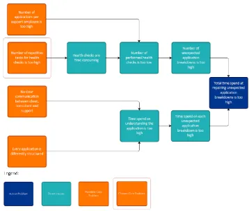
The found core problem is “number of repetitive tasks for health checks is too high” and will be solved by investigating the possibilities of machine learning. I identified the core problem by finding direct causes to the action problem and expending these with associated direct causes until no more causes were found, these causes together form a so-called problem cluster (Heerkens & van

Winden, 2012). This problem cluster is shown in Figure 1.

The problem cluster shows the four possible core problems I found to solve the action problem. It turns out the formulation the action problem time related two direct causes to the action problem were found, instead of one direct cause if I had chosen for a number related action problem. The two found direct causes are “the number of breakdowns is too high” (number related) and “the time spend on each breakdown is too high” (time-related). I expanded both direct causes with other causes, which in the end yielded two possible time-related core problems and two possible number-related core problems. To show the connection between the possible core problems and the action problem I chose to describe the relation from core problem to action problem. This will give a better understanding of the connection between the two than when the connections are explained from action problem to core problem.

The four possible core problems that were found are:

1. Number of applications per support employee is too high.

[image:11.595.109.468.169.473.2]

Monitoring and maintaining over a hundred applications is quite significant for three support employees. As every day some applications break down they have to spend time repairing the applications instead of monitoring them. This means that fewer applications

(12)

11 are maintained and therefore the problems are not spotted and breakdowns not prevented. This results in more applications breaking down.

2. Number of repetitive tasks for health checks is too high.

The health checks are similar for different applications. As there are over a hundred

applications to maintain this is a lot of repetitive and time-consuming work. This means that the available time for performing health checks is not efficient. Therefore a lot of

applications are not monitored even if some time is available for health checks. This results in more applications breaking down.

3. No clear communication between client, consultant and support.

The lack of communication between the client, consultant and support is two-folded. On the one hand, the lack of communication between the client and support results in a lot of time wasted on understanding the exact problem of the breakdown. On the other hand, the lack of communication, in the form of feedback, between the consultant and support leads to minimal changes in the application building process. This causes high time requirements for solving application breakdowns

4. Every application is differently structured.

There is no uniform application building structure. Therefore applications are differently structured and more time is needed to get an understanding of the cause of the breakdown. This causes high time requirements for solving application breakdowns.

One of these four possible core problems had to be chosen as core problem for this research. This decision is based on the impact that a solution for each possible core problem has on the action problem. The one possible core problem with the highest impact is chosen as core problem of this research.

After talking with the manager of the support department it became clear what the options were. Even though every application is (slightly) differently structured and there is no clear communication between the different parties, the solution would be some sort of a uniform standard within the company for both problems. However, the impact on the action problem from both possible core problems would not be that high, as the amount of time spent on understanding the application is not significant compared to the amount of time needed to repair the number of applications that breakdown according to the support manager’s expertise.

This leaves two possible number-related core problems to be discussed. Hiring more employees would reduce the application per employee ratio, but there is no intent to significantly increase the number of support department employees as it is not in line with the innovation plan of the support department.

This left finding a solution for the possible core problem “number of repetitive tasks for health checks is too high” as most impactful of the four possible core problems. This core problem has been investigated to solve the action problem of the support department. The support department is already working on a new monitoring dashboard to have access to the real-time health of the

(13)

12

Section 1.5: Research objective

The design artefact will be a decision tree that provides guidance to the support department on implementing suitable machine learning algorithms. The decision tree will focus on the two most commonly used types of machine learning, the supervised classification algorithms as well as the unsupervised anomaly detection algorithms.

The possibilities of implementing machine learning algorithms in the monitoring and maintaining processes of the support department will be investigated. However, due to the limited time for this Bachelor Thesis providing a working machine learning code that can be implemented is not feasible. So instead a decision tree that guides the support department in integrating machine learning algorithms will be provided. This decision tree will be universal so other practitioners besides CAPE

Groep’s support department can use this guiding artefact to implement suitable machine learning

algorithms in their information systems. As machine learning is a broad topic and limited time is available I had to limit the decision tree to the two most used machine learning types, supervised classification and unsupervised anomaly detection. The used methodology of creating this decision tree is shown in Appendix A and the knowledge questions that needed answering are shown in Appendix B.

To give adequate recommendations to the support department I will apply the created decision tree to the situation of the support department. This will yield a list of missing requirements and steps to take in order to implement machine learning algorithms in the monitoring and maintaining of the applications.

Section 1.6: Measurement of the Solution

Once the given recommendation, originating from applying the decision tree, are processed and the right data is available to implement machine learning in the support departments information systems the number of unexpected application breakdowns should reduce. This can be measured by counting the number of breakdowns per project, which can consist of multiple applications, and compare this to the number of breakdown per project of previous years. When the number of breakdowns is less than the years before the implementation of machine learning did most likely have a positive impact on the number of breakdowns. However, as these are yearly based statistics and the implementation will not take place during the executing of this research it will not be possible to measure the effectiveness.

Section 1.7: Motivation

Reducing the number of application breakdowns is important for both the support department and

the clients. The support department is every day busy with “day-to-day firefighting” which requires

so much time that other responsibilities might not be performed. However, this “day-to-day

firefighting” impacts the client's processes as the applications cannot be used while a breakdown is occurring. To increase the importance of this problem even more, most of the applications are used

(14)

13

Ch2: Literature Review

Section 2.1: Machine Learning

There are four different types of machine learning, however, I chose to focus on the two most commonly used types, supervised machine learning and unsupervised machine learning. In advance to shortly describing these four machine learning types, and going in-depth on supervised and unsupervised machine learning later on, I will thoroughly explain the concept of machine learning. The CEO of Emerj, a company that has knowledge on the impact of artificial intelligence in

businesses, formulated the following aggregated definition of machine learning based on the expertise of several companies (i.e. Nvidia) and Universities.

“machine learning is the science of getting computers to learn and act like humans do, and improve

their learning over time in autonomous fashion, by feeding them data and information in the form of observation and real-world interactions.” (Faggella, 2019)

So, basically, the concept of machine learning is teaching a computer how to learn from data and let it predict or detect patterns/outcomes which makes the job of the user easier. There may only be four main machine learning types, but together they contain a lot of different methods (see Figure 3).

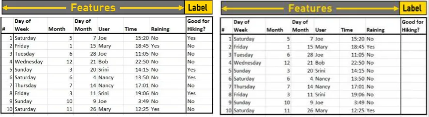
[image:14.595.79.517.355.542.2]

As Figure 3 shows there are machine learning types that require target variables and some that do not require target variables. Target variables are labelled feature sets. When no target variables are required no labelled data is needed. Table 1 shows the difference between labelled and unlabelled data.

Figure 2: machine learning Types (Ivan, 2015)

[image:14.595.81.524.648.769.2]

(15)

14 Labelled data consists of a set of features together with an indication of that data, the label. In Table 1 the labelled data is whether or not the day is good for hiking or not. If the data does not contain a label that gives an indication of that data it is called unlabelled data. The rest of the section will describe the different types of machine learning.

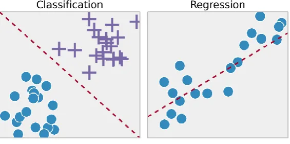
First, there is supervised machine learning. This type of machine learning needs labelled data in order to accurately label a new feature set, by either classifying new feature sets (classification) or predicting the value of new feature sets (regression), both are shown in Figure 4. The best way to show the classification approach is to use a popular example, the Titanic: machine learning from Disaster challenge on Kaggle.com. They provide a dataset with all sorts of passenger data (i.e. age, sex and travel class) together with the information if the passenger survived the disaster or not. By using classification the algorithm will try to find a pattern in the provided dataset to learn what criteria have the most influence on whether a passenger survived or not. The written machine learning code will be tested on another dataset, without the survival information, and predicts whether or not a passenger would have survived the disaster (Kaggle, 2012). Another frequently used application of classification is Medical Imaging, where classification is used to predict whether a tumour is malicious or not. A frequently used example of the regression approach is house pricing. The data contains several house features (i.e. size, number of bedrooms, location) as well as the selling price of the house. This data is used to teach the computer what feature values lead to what selling prices and it will, therefore, be possible to predict the selling price of a house based on a feature set alone (Ng, 2017).

The second type of machine learning is unsupervised machine learning. Contrary to supervised machine learning there is no labelled data present and therefore the classification and regression methods do not work. This type is split in clustering and association. When clustering the machine learning algorithm tries to split the data set in two or more clusters based on the given dataset. There are a lot of applications for this type of unsupervised learning, for instance, it can be used for data reduction by finding representatives data points for homogeneous groups, finding useful and suitable groupings for data classes and it can be used to find unusual data points (Priy Surya, 2019). When using association the machine learning algorithm tries to mine and extract rules and patterns from the dataset to explain the relationship between the different features. This is often used to get

insight into businesses’ and the organisation’s huge data repositories (Ivan, 2015).

[image:15.595.157.440.377.517.2]

Then there is semi-supervised machine learning which is a combination of supervised machine learning and unsupervised machine learning, therefore, it uses both classification and clustering. This type is most often used for voice recognition and web content classification (Rodriquez, 2017).

(16)

15 Finally, there is reinforcement learning which can be used both on labelled data and unlabeled data. Reinforcement learning works differently from the other types of machine learning as reinforcement learning uses a reward system. By subjecting an agent to an environment and rewarding or

punishing the agent based on certain actions the agent will learn what is expected of him. By using this approach the computer will be able to learn how to drive a car, finding the shortest way through a maze and learning how to play a video game (Simonini, 2018)(Ng, 2017).

Section 2.2: Supervised Classification Machine Learning

There are a lot of supervised classification algorithms available and they all need labelled data to gain an understanding of the data and start predicting errors. Every algorithm has benefits and disadvantages and based on the available data one algorithms might perform better than another. The supervised classification algorithms that will be discussed are general and frequently used by practitioners. This does not mean that these are the only algorithms that have to be considered during training and testing. They can, however, be used as a starting point for machine learning as some will have pretty decent accuracy for the data the practitioners might have available. The following algorithms will be described. Decision Tree, Naive Bayes, k- Nearest Neighbours (kNN), Random Forest, Neural Network (Sidana, 2017)(Raina & Shafi, 2015).

Section 2.2-a: Decision Tree.

The Decision Tree structures the data in the form of a tree with decision nodes, moments where a decision has to be made, and leaf nodes, which shows the final classification based on the decision. By going through this created decision tree the algorithm will determine the new label by making decisions at the decision nodes, like did the CPU usage transcend 10%.

Section 2.2-b: Naive Bayes.

The Naive Bayes classifier assumes that every feature of a data set contributes an equal amount to the probability. The algorithm does not take the connections between features into account which makes this one of the simplest algorithms for supervised classification. Because of the simplicity of the algorithms, it is perfectly suited for very large data sets and practise shows that it can

outperform highly sophisticated classification methods.

Section 2.2-c: k- Nearest Neighbours (kNN).

The k- nearest neighbour tries to learn how to label new feature sets based on the labelled data. This is done by looking at the label of the nearest neighbours of a feature value of a new feature set. Every label found adds to that label count of the feature set and the label with the most, so-called,

votes is set as the label of this new feature set. The value of “k” determines how many neighbours are taken into account for each feature value.

Section 2.2-d: Random Forest.

The method, like the Decision Tree, creates decision trees based on the labelled data. However, this algorithm creates multiple decision trees and outputs the label that was outputted by most of the decision trees for a new feature set.

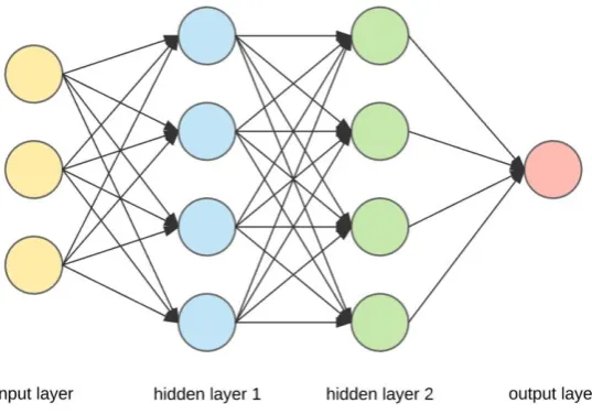
Section 2.2-e: Neural Network.

(17)

16

Section 2.3: Unsupervised Anomaly Detection Machine Learning.

There are a lot of different sorts of unsupervised machine learning approaches, but the anomaly detection method of Andrew Ng of Stanford University stood out. This method is used when

(almost) no labelled data is available and the data comes from machines or applications, which suits

the support department’s information systems.

Anomaly detection is a machine learning method where, based on “normal behaviour” data, the

algorithm tries to find “anomalous behaving” feature sets in a new data set. This approach is based on the Gaussian distribution, also known as the normal distribution. It calculates the mean, called mu, and standard deviation, called sigma, for each feature of a large data set. As the data set contains a lot of feature sets it is not a problem if some “error data points” are present in the data

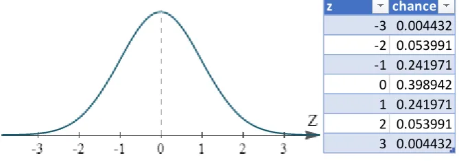
set as it will get filtered out. However, when too many error data slips into the data set the whole distribution changes and the algorithms might not detect the right anomalies. According to Andrew Ng also features that are not following the Gaussian distribution can be used for this approach, however, a Gaussian distribution is preferred (Ng, 2017). The course of Andrew Ng of Stanford University covers two approaches, the Univariate and Multivariate Gaussian distributions. When learning about these two approaches a third, somewhat similar, approach was found, called the Mahalanobis distance. As these algorithms differ from each other they are all discussed in the following three sections. All these three algorithms are based on statistics and therefore an overview of the used statistics can be found in Appendix C.

Section 2.3-a: Anomaly Detection: Univariate Gaussian distribution.

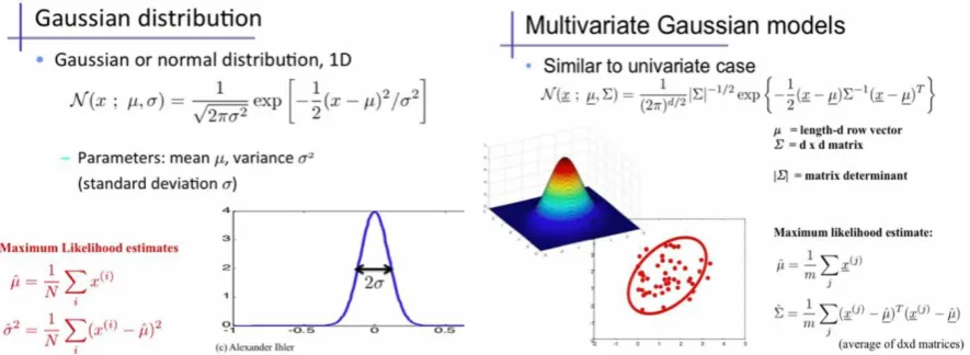
The Univariate Gaussian Distribution uses the mean and standard deviation of each feature to determine the probability of a feature value occurring. Figure 6 shows the formula of calculating the probability of a feature value occurring as well as the statistical ways to determine the mu and sigma.

[image:17.595.163.432.72.260.2]

After calculating the mu and sigma for each feature it will be possible to calculate the probabilities of new feature values with the formula shown in Figure 6. Once the probabilities of all feature values of a new feature set are calculated, the probability of the whole feature set can be determined by multiplying all of the feature probabilities. Then this probability is compared to the value of epsilon, see Appendix D-b for a determination of the epsilon value. When the probability is lower than the epsilon the feature set is detected as an anomaly by the algorithm. An example algorithm can be found in Appendix E-a.

(18)

17

Section 2.3-b: Anomaly Detection: Multivariate Gaussian Distribution.

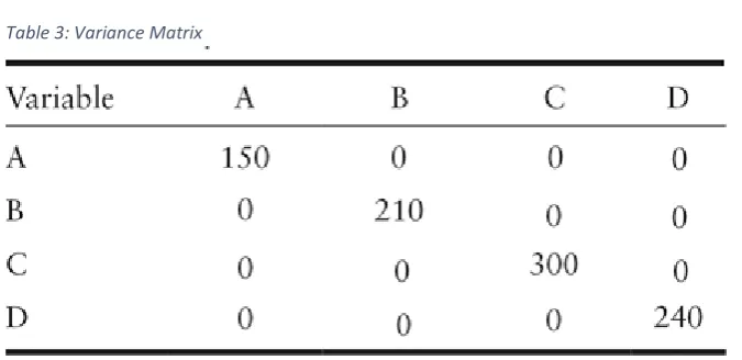
The Multivariate Gaussian distribution is closely related to the Univariate Gaussian distribution with one slight variation. Instead of calculating the probabilities of a new feature value individually and multiplying them afterwards, it calculates the probability of a feature set occurring in one go by using the covariance matrix of the features. The covariance does not only contain the variances of each feature but also the correlation between two features. The formula, as well as the calculation of the mu and covariance matrix, are shown in Figure 7.

The mu is calculated the same for the Univariate and Multivariate Gaussian distribution. However, the sigma of the Univariate Gaussian distribution is changed to the covariance matrix for the Multivariate Gaussian distribution.

The added value of the Multivariate Gaussian distribution compared to the Univariate Gaussian distribution is shown in Figure 8.

[image:18.595.79.522.76.238.2]

Whereas the Univariate Gaussian distribution draws circles over the feature sets, the Multivariate Gaussian distribution also takes the correlation between the different features into account. This is shown in the ellipses around the feature sets. As the figure shows based on the correlation of the two features the red dots should have been spotted as anomalies. As the Univariate Gaussian distribution lacks the correlation of the features it did not spot the anomalies, but the Multivariate Gaussian distribution did spot them.

[image:18.595.100.495.478.657.2]

Figure 6: Univariate Gaussian Distribution (Ihler, 2012) _{Figure 5: Multivariate Gaussian Distribution (Ihler, 2012)}

(19)

18 There are also a few other things to take into account when choosing between Univariate Gaussian distribution and Multivariate Gaussian distribution. When using the Multivariate version of the Gaussian distribution the number of features may not be too large as more features require more computational power. The reason for this is that the inverse of a matrix has to be calculated and larger matrices are harder to invert than smaller matrices. Also, the dataset of the Multivariate Gaussian should be at least ten times bigger than the number of features to get good values. Besides, when the number of features is bigger than the dataset, this option is impossible to use as than the matrix is not invertible. An example algorithm can be found in Appendix E-b.

Section 2.3-c: Anomaly Detection: Mahalanobis Distance.

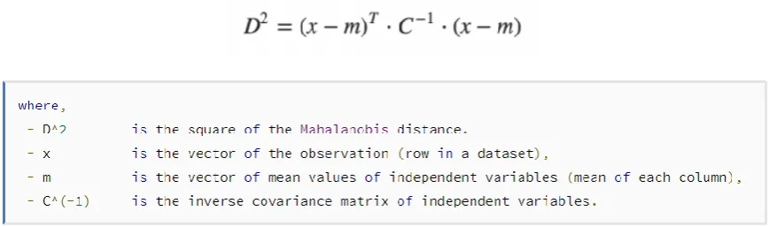
The final researched algorithm is the Anomaly Detection: Mahalanobis Distance. This method uses the mu and covariance matrix of the different features to calculate the Mahalanobis distance that a feature set is away from the centre of the dataset. The formula for the Mahalanobis distance can be found in Figure 9 (Machine Learning Plus, 2019). See Appendix E-c for an example code.

[image:19.595.79.518.328.456.2]

This Mahalanobis distance value is then compared to the chi-square test with (number of features minus one) degrees of freedom and when the Mahalanobis distance surpasses the chi-square test value it is detected as an anomaly. The Chi-square values can be found in Table 2.

Figure 8: Mahalanobis Distance Formula

[image:19.595.213.413.539.768.2]

(20)

19

Ch3: Solution design

During this chapter, I will explain my solution design by first introducing the chosen design artefact in section 3.1. Then in section 3.2, the created design artefact is discussed step by step in full detail.

Section 3.1: Design Artefacts

As design artefact, I created a decision tree that goes both over the requirements for predicting errors, supervised classification, and detecting anomalies, unsupervised anomaly detection. The decision tree is designed to be neat and simple, so far that it is possible for a challenging subject as machine learning. I tried to keep the number of steps and number of words as low as possible to keep the decision tree clear and consistent. The decision tree is based on information gathered during literature studies, as addressed in chapter 2. The rest of this chapter is all about explaining the created decision tree.

Section 3.2: Decision Tree

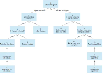
[image:20.595.83.523.354.672.2]

The created decision tree will be explained by addressing all the steps it contains subsequently, first for predicting errors and then for detecting anomalies. The whole decision tree is shown in Figure 12.

(21)

20 1. What is the goal?

By answering this question the machine learning type is chosen and the corresponding requirements and approach to implementation are given during subsequent steps. When predicting errors is the intended use of machine learning step two will be next, if detection anomalies is the objective step nine will be next.

2. Is labelled data available?

Labelled data is the key requirement for supervised classification and therefore of utmost importance. When no labelled data, as mentioned in section 2.1, is available it should be gathered. To get the practitioner started on labelling the data some labelling techniques are given at step three of the decision tree. If the data is already labelled step four will address the balance of the labels in the data.

3. Label the data.

Gathering labelled data is a time-consuming, effortful and challenging endeavour. It not only requires the expertise of a frequent user of the data, or application/machine which produces the data, but also machine learning knowledge and experience to adequately direct the experts on gathering/labelling the data. There are several methods that help with labelling data. The practitioner should decide whether to use one of these methods or find some other labelling approaches to gather labelled data as every data set is different and might need a different labelling method, that might not be mentioned here. Several methods of labelling data, with their pros and cons, that might help the practitioner start with gathering labelled data are (Altexsoft, 2018):

• Internal labelling:

Assign an in-house team to the task. This ensures high accuracy of the labelled data as the team knows the data and its current use. It also will be possible to track the labelling progress as the labelling is done within the company. However, this labelling requires a lot of time, which might result in high costs, and lack of machine learning knowledge within the team might lead to inefficient labelling.

• Outsourcing:

Recruit temporary employees to label the data. This makes sure that the right skills for the labelling team can be gathered to effectively label the data. However, the newly assembled team needs an organized workflow by a manager to execute their tasks.

• Crowdsourcing:

Cooperate with freelancers from crowdsourcing platforms. This will reduce the cost of labelling data, as the freelancers are funded by multiple companies/people. The freelancers are also experienced in labelling the data so it will not take too long to get results. However, as the freelancers are not an employee of the company the results might have less quality than intended.

• Specialized outsourcing companies:

Hire an external team to label the data. As a specialized company is hired the results have a high quality, as defined in the contract. However, the costs of hiring an external company to label the data are often quite high.

• Synthetic labelling:

(22)

21 available data. This will ensure that no third party will get hands-on sensitive and regulated data. This will also make the training of the algorithms easier as there are no mismatches and gaps in the data. Overall this is a cost- and time-effective method of labelling the data. The big downside of this approach is that high computational power is required.

• Data programming:

Use scripts to label the data. This is an automated process and yield fast results. However, the quality of the data set will be less then experts labelled the data.

No matter what type of data labelling will be used it is recommended to have an employee with machine learning experience overlooking/guiding the process to ensure the desired labelled data is gathered. Before a deeper look is taking into the labelling of the data it is important to look at subsequent steps of this decision tree to see how the data is used and what other requirements there are. It might be possible to gather several requirements during one data-gathering session.

4. Is the data balanced?

The data should contain both feature sets with errors/breakdowns and feature sets that behave normally. However, when one of the feature sets contains way more samples than the other the algorithms will have trouble predicting. Even though, there is not a formally defined distribution that indicates an imbalance in the data the rule of thumb is that a data set is imbalanced when the labelled feature sets have a 1:10 ratio (Datascience, 2016). This means that when there are ten times as many feature sets of one label than another it is said to be imbalanced and therefore would benefit from balancing techniques. When the data is imbalanced step five will provide some balancing methods to investigate. When the data is balanced enough the training of the algorithms is explained at step six.

5. Balance the data.

There are several methods to counter imbalance in data but, just like with labelling the data, there is no uniform way to do this. Some methods that are worth investigating are (for detailed explanation the article “Fighting Imbalanced Data Set with code Examples” (Wei, 2019) might be useful):

• Gathering new, most likely error, data examples.

Often the imbalance comes from the lack of error examples and therefore gathering some extra would be helpful to balance the data. However, in most cases, this is not possible as encountering an error would have significant impact on the company and other people (e.g. an aeroplane engine or assembly line failing).

• Methods to level the data.

It is possible to changes the number of feature examples to achieve a more balanced distribution. Some examples, with their pros and cons, are:

o Under-sampling.

By reducing the number of data samples of the majority feature set(s) a more balanced distribution can be attained. This also reduces the run time of the algorithms and needed storage capacity for the data, however, it might also cut feature samples that contain important information for the algorithms and reduces their effectiveness.

o Over-sampling.

(23)

22 more balanced distribution can be attained. This eliminates the downside of under-sampling as no data is deleted, but might lead to overfitting since feature data is replicated.

• Algorithms to level the data.

Algorithms can be used to modify the bias towards majority feature sets of the selected machine learning algorithms. This is a challenging method to use and therefore it requires a good understanding of both the current machine learning algorithm as well as the by algorithms modified version. Also, the precise reasons why the machine learning algorithm is failing to use the current data distribution is needed. The most used algorithms are cost-sensitive approaches.

o Cost-sensitive approaches.

This type of learning algorithms take the misclassification costs, and possibly other types of costs, in consideration and tries to minimize the total costs of the predictions. This method is explained in-depth in “Cost-Sensitive

Learning and the Class Imbalance Problem” (Ling & Sheng, 2008).

• Weight the labels.

By adding weight to the labels, to indicate their significance, the algorithm will adjust its predictions accordingly. However, assigning the right weight to the label(s) is not an easy task and will require experience and expertise of machine learning.

If none of these methods are of any help to attain a more balanced distribution a study in other methods will be necessary. There are countless methods to balance data and an applicable method might be found this way. Once the data is balanced enough a start can be made with training the algorithms, explained at step 6.

6. Train algorithms.

Now that the right data is at hand the algorithms can be trained. This is often done by splitting the available data into two sets, the training set that contains 90% of the data and test set that contains 10% of the data. Make sure to randomly shuffle the data beforehand. This will ensure that the error examples are better distributed over the whole data set, as it will split the, often clustered, errors. Then it is time to train the different classification algorithms, some good algorithms to start with are:

• Decision Tree.

• Naive Bayes.

• k- Nearest Neighbours (kNN)

• Random Forest

• Neural Network.

These algorithms are explained in sections 2.2-a to 2.2-e. Once the algorithms are trained the practitioner should go to step five to compare the performance of the algorithms with different number of features. The evaluation and feature selection of the algorithms, as addressed in step seven, has to be done after the algorithms have been trained.

7. Compare algorithms.

The evaluation and feature selection of the algorithms are done by calculating the f1-score by testing the algorithms on the test set, explained in Appendix D-c. By calculating this f1-score of all algorithms with different sets of features for each algorithm the best

(24)

23 the highest-scoring feature combination of each algorithm, should be compared. The

algorithm with the highest f1-score, that contains that algorithms best feature combination, will be chosen as the best algorithm for this data. When the best performing algorithm is found it should be implemented, as shortly described in step eight.

8. Implement the algorithms.

The implementation of the best performing algorithm is different for every dataset. There are, however, a few things to keep in mind while implementing the algorithm.

• Access to real-time data.

The algorithm should have access to the real-time data to predict the errors as quickly as possible because the longer it takes to predict the error the longer it will take to handle the error.

• Attach an alarm.

The algorithm will start predicting errors and therefore an alarm should be attached to an error prediction so it is known when an error is expected. Then the predicted error can be inspected and, when predicted correctly, fixed.

• Evaluate the algorithm.

By checking whether or not the algorithm accurately predicts the errors valuable information is gathered. Based on the performance of the algorithm the decision to adjust it or not can be made.

• Consider automatically updating the training set.

In some cases, the system/machine data will evolve over time and will gain or lose certain errors. This means that, when the algorithm did not get updated while the system/machine evolved, the algorithm might start predicting errors when nothing is going on and not predict errors when something is going on. By updating the training data of the algorithm this can be prevented. However, it is also possible that a change in the data is indeed a developing harbinger. When the training set is being updated with this data it will learn that this change is not worrisome and therefore not worth predicting. It depends on the available data and the reason for

implementation when automatically updating the algorithms is useful. Automatically updating the training set should be thought of by each machine learning

implementation.

9. Is normal behaving data available?

Unsupervised anomaly detection does not need labelled data to train the algorithms. Instead, these type of algorithms needs normal behaving data to learn when the system/machine is working as intended. Therefore a data set that only contains normal behaving feature sets is needed. If this data is available the next requirement should be checked at step eleven. If this data is not available step ten should be investigated.

10. Gather normal behaving data.

(25)

24 the data as described at step three as both data requirement will be fulfilled this way. When only normal behaving data is needed a combination of logs and graphs might help filter the errors out the training set, however, these logs might be based on thresholds and therefore not yield the right data. An expert of the data source will be needed to successfully

categorize data moments as anomalous and non-anomalous. Before this data should be gathered the follow-up steps should be investigated to find out if some other requirements are missing. Then the gathering of the normal behaving data and the other requirement might be done at the same time to reduce the time spent on implementing algorithms in the Information System. When the normal behaving data is gathered checking for error

examples is done at step eleven.

11. Are there some error examples available?

The algorithms can be trained with the normal behaving data, however, in order to evaluate and attain the right features and epsilon value some error data is needed for testing. A ratio of 10.000 normal behaving data to 20 error examples, so 500:1 normal behaving to error examples, is a good guideline (Ng, 2017). When there are enough error examples present the training of the algorithms can start at step thirteen. However, when this is not the case some error examples should be gathered as explained in step twelve.

12. Gather some error examples.

In order to evaluate the performance of the algorithms and find the right features and epsilon value, some error examples are needed for the calculation of the f1-scores. This gathering can be done by purposely letting the data sources breakdown, but this is not an advisable method of attaining the data as this might have significant consequences for the company and or users. A better way to attain this data is to go through the logs and graphs of the data and gather the data of the moments an error occurred. This sounds easier than it is in practise as several difficulties might show up, as can be seen in section 4.1. It will be beneficial if the error examples have different error reasons, for instance some with a memory-related error and other with a CPU related error. This way the algorithms will be tested on multiple errors which will result in a more applicable implementation in the end. When there is no way of gathering error examples the algorithms can also be trained on the normal behaving data and their performance can be evaluated after implementation by keeping track on its detecting accuracy. The best performing algorithm can then be kept and the others can be left out. When some error examples are gathered or the evaluation after implementation method is chosen the algorithms should be trained as described in step thirteen.

13. Train the algorithms.

The algorithms should be trained on about 60% of the normal behaving data and the other 40% and error examples will be used for the evaluation of the algorithms (Ng, 2017). The three researched algorithms for unsupervised anomaly detection are:

• Univariate Gaussian.

• Multivariate Gaussian.

• Mahalanobis Distance.

(26)

25 distributed can also be beneficial for the detection of anomalies (Ng, 2017). When the algorithms are trained the should be evaluated and compared as explained in step fourteen.

14. Compare the algorithms.

For the evaluation of the algorithms, and feature and epsilon selection, the f1-score will be calculated as explained in Appendix D-c. By calculating the f1-score of all algorithms with different features and epsilon values the best combination, the combination that yields the highest f1-score, for the data will be found. Then by comparing the highest f1-scores of the different algorithms the algorithm that is best aligned with the data can be used and implemented as step fifteen indicates.

15. Implement the algorithms.

The implementation of the best performing algorithm is different for every dataset. There are, however, a few things to keep in mind while implementing the algorithm.

• Access to real-time data.

The algorithm should have access to the real-time data to detect anomalies as quickly as possible because the longer it takes to detect the anomaly the longer it will take before investigation is started and the possible problem is

prevented/addressed.

• Attach an alarm.

The algorithm will start detection anomalies and therefore an alarm should be attached to get notified whenever an anomaly is detected. Then the predicted anomaly can be inspected and, when detected correctly, addressed.

• Evaluate the algorithm.

By checking whether or not the algorithm correctly detected the anomalies valuable information is gathered. Based on the performance of the algorithm the decision to adjust it or not can be made.

• Consider automatically updating the training set.

In some cases, the system/machine data will evolve over time and the definition of an anomaly might change.

(27)

26

Ch4: Data analysis

Section 4.1: Data analysis

During an intensive data analysis, the following was found:

• Data accessibility.

The accessibility of the data at the start of my data analyse was not optimal. I could only gather small features sets at a time and had to go through large text files that contained the logs. This is sufficient when the time of a breakdown is known and its cause has to be investigated, however, it makes gathering large sets of the data challenging. Luckily the support department was already improving the data accessibility when my Thesis started and I could access the data easier vis the new dashboard and underlying data architecture (Appendix F).

• Aggregated data saving.

In order to use machine learning, it is important to have as many feature sets with a constant time elapsing between two feature sets. However, the available data was being aggregated. This means that, for instance, the one-minute feature sets became aggregated to a five-minute feature set after three hours had passed. In order to get a large data set with all one-minute feature sets the data should be gathered every three hours, which is infeasible for gathering a large data set. So during this analysis, I ensured that the

aggregating of the feature sets got postponed from three hours to three months so I could gather larger amounts of one-minute feature sets.

• Application features with different times between data points.

Some feature of the applications outputted their feature values every one minute while other features outputted their feature values every five minutes. These outputs cannot be used together for machine learning and therefore the time between feature outputs should be the same for all features.

• Error moments give empty feature sets.

Whenever an error occurred that broke an application down the feature sets were, logically, empty as no data can be gathered when an application is down. That is why I investigated the one-minute feature sets before a breakdown to find a cause for the breakdown. Unfortunately, the inspected feature sets did not show any spikes in the data that could have caused the breakdowns. So I was not able to gather any breakdown feature sets during this research.

• No normal behaving data.

(28)

27

Ch 5: Solution tests

This chapter starts with an introduction to the solution test in section 5.1 before both branches are addressed in sections 5.2 and 5.3, supervised and unsupervised respectively. I conclude this chapter with a comparison between both outcomes and determine which type has more potential for the support department.

Section 5.1: Solution Test Introduction.

The support department of CAPE Groep can, in principle, use both supervised and unsupervised machine learning in monitoring and maintaining their applications. Supervised machine learning might be able to predict future breakdowns, by training the algorithm(s) on the data before breakdowns happened in the past and then use the trained algorithms on real-time data.

Unsupervised machine learning might be able to detect anomalies that cause breakdowns that the

current thresholds do not detect, by providing a “normal behaving” dataset to the algorithm(s) it

uses this information to spot differences between the provided data and the real-time data. In order to find out which type of machine learning is better applicable to the available or gatherable data, both branches will be investigated, in sections 5.2 and 5.3, and compared afterwards in section 5.4.

Section 5.2: Solution Test Decision Tree: Supervised Branch.

For implementing supervised classification in their information system the support department of CAPE Groep has to label their data as well as balance this labelled data. However, before this can be done the support department should conduct a research on breakdown data. If breakdown data is indeed gatherable the labelling and balancing of the data can begin.

The first question to be answered in the predicting breakdowns branch is “Is labelled data available?”. Based on the conducted research, addressed in chapter 4, the answer to this first question is that the Mendix application data is not labelled. The breakdown moments do not contain feature values as the application is down and no data can be collected. When investigating the feature sets directly before a breakdown no significant change in the data was found as an indication of the upcoming breakdown. However, as the support department is in the middle of improving its monitoring and maintaining capabilities with the new dashboard and data architecture the data accessibility was not optimal during this research. It might turn out that when a new investigation in the data before a breakdown is conducted signs of the future breakdown can be found. This due to the fact that the data is better accessible as well as more applications can be investigated. When this is the case the data can be labelled and then be used for supervised classification. However, there is no guarantee this will be possible.

The next question, assuming labelled data can be gathered in the future, that arises is “Is the data balanced?”. When looking at the collected data it turns out that, even for applications that regularly breakdown, the number of feature sets that are not close to breakdowns of applications is

significantly higher than the number of feature sets that are close to breakdowns. One of the datasets I investigated went out of memory 20+ times during one day and even then only 17.48% (501) of all its feature sets (2866) was within 15 min. of a breakdown. So around one-fifth of all feature sets of an application that regularly breaks down might be used as breakdown information.

So for the applications that do not regularly breakdown the “normal data” “breakdown data” ratio

(29)

28 So before the training, testing and implementation of supervised classification algorithms can start the support department will have to label and balance its data. In order to get the right data, the support department will have to conduct a research into the gathering breakdown examples. When these two main requirements for supervised classification are met the training, testing and

implementation of the algorithms should pose no real difficulties.

Section 5.3: Solution Test Decision Tree: Unsupervised Branch

In order to implement unsupervised anomaly detection in the support department’s information

systems, they have to gather a lot of non-anomalous feature sets and test the algorithms on real-time data.

The first question that arises when going through the unsupervised branch of the decision tree is “Is normal behaving data available?”. The data research of chapter 4 showed that, when the logged errors and breakdowns are excluded from a data set, the remaining data still contains spikes. This makes it hard to find out whether or not this data should be categorized as non-anomalous data or not. However, a group of experts within the company should be able to classify these data spikes.

The next question of the decision tree is “Are there some error examples available?”. As there are no feature values during breakdowns and the feature sets prior to the breakdown do not provide clear changes there are no clearly defined anomalous feature sets available. The lack of anomalous feature sets makes testing of the algorithms with a test set not possible. However, the testing of the algorithms can also be done with real-time data. By implementing the trained algorithms on the real-time data it will start detecting anomalies. Then these anomalies can be investigated by the support team to see if there was actually an error or breakdown. Based on the results the algorithms could be tweaked to represent the real-time data better.

So before the support department can implement anomaly detection algorithms they have to narrow down when the applications are behaving normal and when not. Then that data should be used to train the algorithms and implement the trained algorithms afterwards. Once the algorithms start detecting anomalies they have to investigate them. Based on these investigations they can determine the usefulness of these algorithms on the real-time data and decide to tweak the algorithms accordingly.

Section 5.4: Supervised vs Unsupervised

As mentioned before, both types of machine learning are, in principle, useful to monitoring and maintaining the Mendix applications. However, the largest encountered difficulty during this research was the lack of breakdown data. This has significant impact on the applicability of the supervised classification algorithms as these algorithms cannot be trained without breakdown data. For the unsupervised anomaly detection the impact is significantly less as the training of the

(30)

29

Ch6: Conclusions and

recommendations

Overall I think the support department can benefit from implementing machine learning algorithms in the monitoring and maintaining of the Mendix applications. However, the available Mendix application data is not (yet) in line with the data requirements for both supervised and unsupervised machine learning. The fact that it was not possible to collect breakdown feature sets and no clearly defined normal behaving data set was gatherable the implementation of either one machine

learning type is infeasible for the moment. However, with the help of the created decision tree, I am able to provide some to the point advice for implementing machine learning algorithms in the future.

Of the two types of machine learning, supervised classification and unsupervised anomaly detection, I would advise the support department to start with unsupervised anomaly detection. The fact that no breakdown data was gatherable makes training of the supervised classification algorithms infeasible. An intensive research in the feature sets before application breakdowns might yield enough breakdown examples. However, as no breakdown examples were found during this research there is no way to guarantee this data will be gathered during a new data investigation. This makes focussing on the supervised classification algorithms a riskier endeavour than to focus on the unsupervised anomaly detection algorithms.

In order to be able to test the unsupervised anomaly detection algorithms on the real-time application data, a non-anomalous data set should be gathered. This can be done by investigating the data peaks of feature sets that are nowhere near to a breakdown. If the support department manages to categorize these peaks in either non-anomalous data or anomalous data a training set will be gatherable. Then the algorithms, some are provided in Appendix E, can be trained on this gathered training set and should afterwards be applied to the real-time data. Based on the

performance of the algorithms a decision can be made to keep them, tweak them or delete them. If the mentioned unsupervised anomaly detection algorithms do not provide the expected outcome of the support department it might be worthwhile to investigate other types of unsupervised machine learning before starting with supervised classification. This because the attaining of the labelled data for supervised classification will be an uncertain and time-consuming endeavour.

(31)

30

Bibliography

Altexsoft. (2018). How to Organize Data Labeling for Machine Learning: Approaches and Tools | AltexSoft. Retrieved September 9, 2019, from

https://www.altexsoft.com/blog/datascience/how-to-organize-data-labeling-for-machine-learning-approaches-and-tools/

Datascience. (2016). classification - When should we consider a dataset as imbalanced? - Data Science Stack Exchange. Retrieved September 2, 2019, from

https://datascience.stackexchange.com/questions/11788/when-should-we-consider-a-dataset-as-imbalanced

Elastic. (2019). Open Source Search & Analytics · Elasticsearch | Elastic. Retrieved August 1, 2019, from https://www.elastic.co/

Faggella, D. (2019). What is Machine Learning? | Emerj. Retrieved July 1, 2019, from https://emerj.com/ai-glossary-terms/what-is-machine-learning/

Google Developers. (2019). Classification: Precision and Recall | Machine Learning Crash Course | Google Developers. Retrieved August 15, 2019, from

https://developers.google.com/machine-learning/crash-course/classification/precision-and-recall

Grafana. (2019). Grafana - The open platform for analytics and monitoring. Retrieved August 1, 2019, from https://grafana.com/

Heerkens, H. (Johannes M. G., & van Winden, A. (2012). Geen probleem : een aanpak voor alle bedrijfskundige vragen en mysteries : met stevige stagnatie in de kunststoffabriek. Van Winden Communicatie. Retrieved from https://research.utwente.nl/en/publications/geen-probleem-een-aanpak-voor-alle-bedrijfskundige-vragen-en-myst

InfluxDB. (2019). InfluxDB: Purpose-Built Open Source Time Series Database | InfluxData. Retrieved August 1, 2019, from https://www.influxdata.com/

Ivan, M. (2015). Types of machine learning algorithms | en.proft.me. Retrieved July 23, 2019, from https://en.proft.me/2015/12/24/types-machine-learning-algorithms/

Kaggle. (2012). Titanic: Machine Learning from Disaster | Kaggle. Retrieved July 1, 2019, from https://www.kaggle.com/c/titanic/overview

Ling, C. X., & Sheng, V. S. (2008). Cost-Sensitive Learning and the Class Imbalance Problem Motivation and Background. Springer. Retrieved from

https://cling.csd.uwo.ca/papers/cost_sensitive.pdf

Machine Learning Plus. (2019). Mahalonobis Distance - Understanding the math with examples (python) – Machine Learning Plus. Retrieved July 23, 2019, from

https://www.machinelearningplus.com/statistics/mahalanobis-distance/

Ng, A. (2017). Machine Learning — Andrew Ng, Stanford University [FULL COURSE] - YouTube. Retrieved July 4, 2019, from https://www.youtube.com/playlist?list=PLLssT5z_DsK-h9vYZkQkYNWcItqhlRJLN

(32)

31 Priy Surya. (2019). Clustering in Machine Learning - GeeksforGeeks. Retrieved July 23, 2019, from

https://www.geeksforgeeks.org/clustering-in-machine-learning/

Raina, H., & Shafi, O. (2015). Analysis Of Supervised Classification Algorithms. INTERNATIONAL JOURNAL OF SCIENTIFIC & TECHNOLOGY RESEARCH, 4(09). Retrieved from www.ijstr.org

Rodriquez, J. (2017). Understanding Semi-supervised Learning - Jesus Rodriguez - Medium. Retrieved September 1, 2019, from

https://medium.com/@jrodthoughts/understanding-semi-supervised-learning-a6437c070c87

Sidana, M. (2017). Types of classification algorithms in Machine Learning. Retrieved September 9, 2019, from https://medium.com/@Mandysidana/machine-learning-types-of-classification-9497bd4f2e14

Simonini, T. (2018). An introduction to Reinforcement Learning. Retrieved July 23, 2019, from https://www.freecodecamp.org/news/an-introduction-to-reinforcement-learning-4339519de419/

Soni, D. (2018). Supervised vs. Unsupervised Learning - Towards Data Science. Retrieved July 23, 2019, from

https://towardsdatascience.com/supervised-vs-unsupervised-learning-14f68e32ea8d

Designing a Machine Learning Decision Tree for Information Systems: A study into the implementation of supervised and unsupervised machine learning methods