TABU:

A.C. Impedance of Single Muscle Fibres

By

Robert Eisenberg

A thesis presented for the degree of Doctor of Philosophy

in the un~versity of London

Department of Biophysics University College London

AoSTRACT

The impedance of single crab muscle fibres was determined with microelectrodes over t~e frequency range 1 c/s to 10 kc/s. Care was taken to analyze, reduce and correct for caFacitative artifact. The impedance of the fibre was analyzed using linear cable theory, tne accuracy of wbich is discussed. The equivalent circuit of the fibre distributed admittance is found in most

cases to have two capacitances, each in series with resistance, and a resistive shunt. In just two fibres only one capacitance shunted by a resistance was found. In several fibres there was evidence of a third very large capacitance.

rhe values of the elements of the equivalent circuit depend on which of several equivalent circuits is chosen. The .circuit considered most reasonable in the light of the anatomical

evidence consists of two parallel branches: a resistance R in e

series with a capacitance Ce; and a resistance Rb in series with a parallel combination of the resistance R and the capacitance C •

m m

The average circuit values for this model are R

=

21 ohm-cm2; e

Ce

=

47

~F/cm

2

;

Rb

=

10.2 ohm-cm2; Rw

=

173 ohm-cm2; Cm= 9.0

~F/cm

2

•

The relation of the equivalent circuit to the fine structure of crab muscle is discussed. R and

m r ~

e · e

TABU: OF CONTENTS

Abstract

AcKnowledgements

Chapter 1:

Chapter 2:

Chapter

3:

Introduction

Theory

Linear Circuit Analysis Cable Theory

Simple Fibre ·Model

Simple Distributed Resistance Model Two Time Constant Model

Two Time Constant, Distributed Resistance Model

Other Two Time Constant, Distributed Resistance Models Curve Fitting Methods

Appendices:

Derivation of the Equivalence Relations Curve Fitting Computer Program

Methode

Procedure

Corrections for Stray Capacitances

Appendices

Derivation of the Cor~ection Equations The Cathode Follower

Error Analysis of the Corrections

Alternative Methods of Parameter Measure~ent

Chapter

4:

Results

Appendix:

Description

Second Group of Fibres Third Group of Fibres

Errors Arising from the Neglect of 'rhree Dimensional Spread of Current

Equivalent Circuits of the Muscle Fibre Distributed Admittance

~valuation of Circuit Parameters Transient ~esponse of Muscle Fibre

The 'l'hree Dimensional Flow of Current

6

Ch:tpter ): Di::;cussion

Relation of Present Observations to Previous 15C Findings

Relation of Electrical Parameters to Muscle 15C Structure

T am very grateful to P. Fatt and G. Falk for their help and encouragement. I am also indebted to the other

members of the Biophysics Depar~ment and to L. Peachey and A.F. Huxley for many stimulating discussions.

I wish to thank J.L. Farkinson, L.J. ~ard,

~. Copeland, E. Ullrich and A.M. Paintin for technical assistance.

This work was done while I was a Graduate Fellow of

the National Science Foundation. I am grateful to the

Chapter 1

INTRODUCTION

The low frequency capacitance of muscle fibres as

~easured with intracellular electrodes is quite large, ranging from

8

~F/cm

2 in frog (Fatt·& Katz,

1951)

to 40

~F/cm

2 in crab (Fatt

&

Katz,

1953a;

Atwood,

1963).

It is difficult to 'ccount for theee large values of capacitance assuming

reasonable dielectric properties of a predominantly lipid sarcolemma. Recently, the large value of capacitance in frog muscle has been explained by attributing the greater part of it to the sarcotubular syete~ (falk

&

Fatt,

1964),

the structure of which is reviewed in Porter,

1961,

and

franzini-Armstrong,

1964.

It seemed of interest to see if the much larger cafacitance of crab muscle could also be attributed in greater part to the sarcotubular system (first investigated by Veratti, 1902, with the light microscope; more recently by Peachey

&

Huxley,

1964,

with the electron microscope).

clltterent HC products if both c~pacitanc~s are in series with resistance. If either of these conditions is fulfilled, the paaaiv~ electrical propdrties of the fibre will reveal the existence of two capacitances.

The passive properties of a linear system can most ~~tlsfactorily be studied by measuring the impedance of the ~yatem to sinuisoidal currents of different frequencies; that

la,

by measuring the relative aagnitude and phase of the

current and voltage over a range of frequencies. The difficulties of separating different time constants make

measurements of thd transient response of a linear system less satisfactory. A detailed analysis of the relative merits of transient and frequency response methods in the determination of the number and size of the time constants of a linear system leads Lanczos

(1957,

p.

279)

to conclude that the difficulty with transient response methods "lies not with the manner

of evaluation (of the time constants from the experimental data) but with the extraordinary sensitivity of the exponents {that is time constants) and amplitudes to very small changes of the data, which no amount of ••.• statistics could remedy.

The only remedy would be an increase of accuracy to limits which are f~r beyond the possibilities of our present measuring devices".

(Comments in b~ac~ets added). In view of this analysis the

Measurements of i~pedance were made over a wide

frequency range. The qualitative features of the data showed

that the equivalent circuit of most crab fibres contained two

capacitances. each in series with resistance. Values of the circuit elements were obtained from the best fit of such an

equivalent circuit to the experimental d~ta. Finally, the

different forms of the equivalent circuit and the values of

the circuit elemente are discussed in rel~tion to the fibre structure.

Chapter 2.

THEORY.

Linear Circuit Analyaie.

·rhe system under consideration is treated as linear and

passive: linear since the values of the circuit parameters are

independent of potential and current; passive since the only

internal voltage source is constant and can be subtracted from

all observed potentials. The theory of systems which fulfill

these requirements is based on the representation of currents

3nd voltages by complex numbers. The theory is valid for

excitations of arbitrary form but the derivation of the system

properties for the general case depends on the use of Laplace

transforms (Kuo, 1962). Our deriv~tion is restricted to

sinuisoidal excitations although the results are in fact Talid

for any excitation if the 'purely im3~nary frequency variable jw (where j

=

~) is replaced by the complex frequency variable s

=

v

+ jw and the complex currents and voltages are interpreted as the Lapface transforms of the physical currents

and voltages.

fhe response of any linear passive system to a

me the excitation after transients have died away. Any

current or voltage in the system can then be written as

{ .

~

·

w-t]

v<.t)::.

v~

C.05

(cvt

+

¢)

~

1? ..

v ...

el-

e~

where t is time; · , and ~,are the phase differences of voltage and current from some reference, and Ref

J

·

denotes the real part of the complex quantity in the brackets. If we split off the time dependence (which is the same everywhere in the system) by defining a complex voltage

V

and complex

current I as

I

=

1 ... ~;.¢'

then the physical voltage and currents are given by

V(t) :

l?ef

V-e}..,i"}

t(t)

Re[I ei-..,j

12

·rhe physical currents and voltages are hardly ever needed in

circuit analysis since the ratios of various complex currents and voltages contain all the information usually of interest

(i.e. the relative phase and magnitude of the physical

quantities). rhe ratio of complex voltage to complex current

is a frequency dependent complex quantity called impedance

Z

,

whose real part is the effective (equivalent) resistance R,

and whose ima~inary part is reactance X

z

y_

I

Ratios of volta~e to volt3ge and current to current as well as their reciprocal quantities can also be defined. The reciprocal of impedance is another complex quantity called admittance Y, with real part conductance g and imaginary part

suscepta~ce b

Y-

--

_{z -}

I

It is important to note that the effective resistance is not the reciprocal of the conductance. The relations between the real

and imaginary I

Y=

--

_z

p~s of the a~~ittance and

. b-

I

4-

+

~

-

-~-

....

-;.~~

-x

b-

"R~

.

+ x~

impedance are given by

(5)

14

rhe impedance of each of the common circuit elements

~-ft be ~oflned by writing its current-voltage relation in

ctctllp.lex form. ·rhe impedance of a resistor of r ohms is then

real, independent of frequency and equal to r; the impedance

ot a

capacitor C is purely imaginary (i.e. purely reactive),

trequ•ncy dependent and equals

.

-a:

_wC

It can be shown that the complex currents, voltages,

.ad impedances all obey Kirchoff's and OO.'s laws. The

~nalysia of the response of a network to an arbitrary excitation

la then carried out as for a d.c. circuit except complex

·tuanti ties are used. (The discussion above is presented in

d•tail in a number of electrical engineering textbooks:

8.g. futtle,

1958;

Le Page

&

Seeley,

1952;

or Guillemin,

1953).

Cable Theory

It is necessary to use cable theory since current

applied to the muscle fibre p~sses along the internal resistivity

of the fibre before it crosses the fibre membrane; in other

words, the current applied produces a potential drop across

15

Figure 2.1

The Muscle Fibre Treated as a Linear Cable

r ., the internal resistivity, andy, the complex distributed admittanc~, ~

refer to the properties of a very small length of the muscle fibre; they

I

t-·~

1..:

-~

.

I

~

~

rhtt rnembrane admittance is said to be distributed along the lOternal resistance. The fibre may be represented as a

linear (one dimensional) cable if as a flrst approximation tho potenti3l at any disb.nce along the fibre axis is assumed

to be the same throughout the fibre interior. (The validity

of this assumption in examined in Chapter

4:

Results). It

is also useful to assume that there are no potential drops in the external medium. This assumption can be tested and is found to be adequate as long as the source of current is not too

focal. Figure 2.1 shows the circuit of the linear cable

incluJing both assumptions. x is the distance along the fibre axis • r. is the internal resistivity per unit length. y is

1

the complex admittance between inside and outside per unit length (called the distributed admittance).

l'he steady state response of this model to sinuisoidal excitation is known (Lef·age & Seeley, 1952). ror current I applied at x : 0 and potential V(x) measured at x (chosen positive), and assuming the fib~e to be lon~ enough so that there is neither current flow nor potential change at the ends, the transfer impedance Z(x) is

where

V(..x)

I

17

(7)

[image:18.638.96.556.61.725.2]

·rhe parameter

r

is discussed in the Appendix to Chapter 4:

rtesults. In these experiments potential was usually measured

close to the point ~here current was applied. For that

case (7) becomes

(9)

An expression relating the effective lumped resistance aad

reactance (R and X) with the distributed conductance and

susceptance (g and b) can be derived by substituting

y z g + jb into (8) and takin8 real and imaginary parts

( 10).

R=

-X

I~ is important to realize that equation (10) contains

two physically distinct sets of variables: R and X, which refer

to the total impedance seen by a source of current at

x

=

0 (the ratio of potential at x

=

0 to the current applied

element of fibre membrane (the ratio of the potential acrose

that element of membrane to the current throu~h it1.

fhe physical difference bet~een these two sets of

parameters can be seen if one compares the effect of a

resistance H in ser~es ~ith the entire current flowing throu~h s

the cable with the effect of a resistance rb in series with

each element of the cable (see rigure 2.2). The effect of

placing a resistance in series with all the current would be

simply to add the positive real constant R to the i~pedance

z.

s

At any frequency the only effect ~auld be to increase the

effective resist3nce by R • If a plot were made of X vs. rt

s

the curve ~ould be displaced by R but its shape would not be s

chan~ed. On the other hand, the addition of a distri~uted

I

r·esistance r b in series \lfith the admittance y = g -+- jb

produces a ch~nge which is frequency dependent (since in

I I )

general both ~ and b are frequency dependent • r'he admittance

y

=

g + jb of an element of membrane consisting of resistance

'

in series with y is

~~

(' +

rb~')

+

(I

+

rbct

)"l.

+

b-19

Figure 2.2

T~o Kinds of Series Resistance

A: the entire fibre impedance in series with the

resistance R •

8

B: the distributed admittance y• in series with the

distributed resistance rb.

All quantities except R refer to a very small length of

s

[image:22.618.64.469.266.509.2]

A

'

IJ

IJ

.

T?s

-

-8

I

rhe addition of a distributed resistance h~s two effects on a plot of X vs. R: first, there is ~ chan~e in the shape of the

curve; secondly, tif the model for y contains no induct3nces)

at very hi~h frequencies the capacit3nces in y have ne~ligible

impedance and the entire pot~ntial drop acrose the fibre

..!. -~,., u •vr .. ·'-Ru.

1\

~embrane is developed across rb. Thus, ~t very hi~h frequencies a plot of X vs. R must bend down to give a pure resistance.

The only mea.sul'ement made here with x ~ 0 ar~ those of the d.c. sp~ce constant _•

7\

is found by setting b

=

0

(the renctance of any linear passive circuit is zero at zero

frequency) in (8):

c \

(12)

-;~ote that 1/g is identical with the total d.c. resistance of the

Jistributed admittance y; it is not necessarily identical with

~ , the resistance of the plasma membrane. Measurements with m

.,T

"o"'-~ro -(' ('fl•JilV>C.. iPS

' r.

finite electrode separation''req:Jire the use of a more complicated

formula (equation

3,

p. 72 in FalK

&

Fatt, 196.~). Such

measurements are not presented here.

rhe basic metnod of this investigation C3n now be seen.

,:mpedance measu.cements were rt\.•ide over .'l wide range of frequencies

data can be used. Ph=tse and magnitude, or resistance and

reactance can be plotted against log frequency (sometimes

called the Bode plot: Bode, 1945) or reactance can be plotted

against resistance (called the Cole-Cole plot: Cole and Cole,

1941). The latter plot is particularly useful in revealing

the qualitative features of the impedan~e function because

mathematically it i s the plot ('mapping') used to sho~ the

behaviour of a complex function (here Z) of a real variable

(w) (see Churchill, 1960}. Although the explicit dependence

f D X f . . . th. 1

\

i

-tt\~

f ti

o n and on requency 1s not g~vcn 1n ~s p ot, ac 1n orma on

is lost since any impedance function is specified (~ithin a

scale factor) if a relation bet·.,een two of its variable is

given (see Bode, 19~5. and Tuttle,

1958,

for proofs and

discussion for lumped circuits; see Macdonald and Brachman,

1956,

for a general discussion of the physical significance of these

relations and a proof that they hold for distributed linear

passive systems). In practice, the scale factor is set bJ

labelling some point of the impedance locus ~ith the

corres-ponding frequency.

The other plot used, that of phase vs. log frequency,

has two advantages: it is sensitive at relatively low frequencies

to changes in values of circuit parameters and it shows random error

24

of phase, not H or A). The p~ots of resistance, m3~nitude of ~mpedance, or reactance against lo~ frequency were found to be

less useful since they were relatively insensitive to model

or parameter changes.

Simple iibre Model.

In a simple model of the fibre y is taken to be a

capacitance in p~allel with the membrane resista~ce r m

(Fig. 2.3). 'rhe expression for the real and imaginary parts

of the admittance are then

(13)

b:.

w

CWl

The d.c. space constant is

( 14)

and the input resistance

(15)

Fieure

2.

3

shows the shape of the impedance locus for this

Figure 2.3

The Impedance Locus ot the Simple Fibr~ Model

·The impedance locus ot th~ circuit in the upper right hand corner is shown.

The circuit elements are identified for use in the text. The scales are

given in terms o! Rin' th~ d.c. resistance. The solid

45°

line represents the line approached at high frequencies by the impedance plots of all

.

1

~ •

1'\1

•

tJO

...

ra.

U"\

1'\1

• 0

X

0

J

~ • 0

~

•

0

U'\

1'\1

•

0

this curve is independent of the actual values of the par~meters

c , r , and r .• This can be seen by writing the equations (13)

m m 1

in dimensionless form.

ca.

r~

=

I

b

rW\:::

-v

where the scale factor r is set by the input resistance, and

m

Simple Distributed Resistance Model.

Another model is that in which the circuit element of the

simple model·is in series with a resistance (Fig. 2.~). This

distributed resiGtance makes the impedance at infinite frequency

purely resistive. The admittance of this model is given by

( 1

+

r-)

+

""A

r

(' +

r)"l.-+-

"'Y>~ r~

where the dimensionless variables

+

(' +

r)"l.

+

lJ

4

r~

r. .

- . ) v=wr~~~"c~

r"" •

have been used. The shape of this locus is seen to depend on

27

rigure 2.4

The Impedance Loci of the One Time Constant. Distributed Resistance Model

The impedance loci of the circuit in the upper rieht hand corner are shown.

Circuit elements are defined for use in text. fhe 45° line represents the

limiting high frequency locus of the circuit for rb

=

0; i.e. in the

ahsence o: distributed resista~ce. The lqrge numbers under the abcissa

give the value of R /H. for each curve. where R , the infinite freqyency

oo

1n oo

resi

s

t~nce,

equals

0.5

(rbri)*. !he small numbers on both axes give the

scales in terms of R . .

on~y one parameter r

=

rb/rm• the s~ale factor rm being set by

the input resistance

The space constant for this model is given by

1

l/~

7\

=

.

[r..,;c:

r.

J

Two Time ~onstant Model.

Another model of the fibre is shown in Fig. 2.5. In

3ddition to the two parallel paths formed by r and c as in

m m

(17)

(18)

the simple models. there is a third path through the resistance

r and capacitance c • The inside-outside admittance of this

e e

model is ~iven by

I+

v~

using the dimensionless variables

If'\

.

rJ

.

t..:• •rl

r,,

1"\,J co <.:r

·-+

.

· (\J

.

r l

.

0 0

X

.::.>

I

c:

·-0:::

\.()

CX)

.

fwo fime Cvnst3nt, Jistributed ~esistance Model.

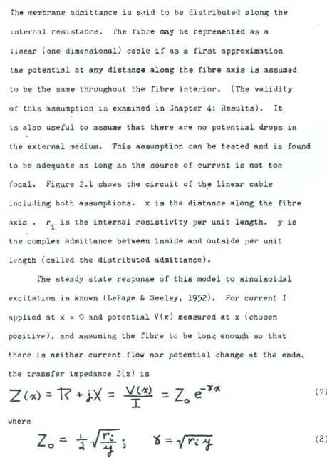
The circuit for this model is shown in Fig. 2.6. This

model 1s the only one which adequately fits ·all the impedance

loci observed. It is sornewh3t more complicated than the two

time constant model, but this complication is required by the

experimental data. The real and imaginary parts of the

admittance of this model are

D

br""'

(20)

with

An Impedance Locus for th~ r~o Time Constant, Distributed Resistance Model

An impedance locus of the circuit shown in the upper ri~ht hand corner is shown.

The locus was calculated for the circuit values C /C ~ 1.5; R / R

=

2.7;

m e m e

-2

-13

Rb/Rm

=

2.4 x 10 ; ce/ri = 7.2 x 10 F/ ohm. The impedance locus ~ould

approach the 45° line through the origin if the distributed serles t·esistance

rb were not present. Scales given in terms of R. • R , the infinite

l.n <D

[image:39.925.157.711.206.451.2]

.

--,

.

' ' •

·'·

Cl1

v

X

I

.

8

1.{\

1\j

•

·:""'

8

v

=

cv c

e.

re. ·

_.)

are used.

It is instructive to examine the behaviour of this model

at high frequencies. !he high frequ~ncy limiting properties of the distributed admittance 3re

---.,..~~ ~

0

j

~c.

....

Jb

(neglected terms differ by factors of w2).

The corresponding limited behaviour of the lumped impedance

is

R-

il (

r .. r .. )

'I

-a.

=

7?_,

-X

Jn other words the resistance remains constant at high

frequencies ~hile the reactance decreases in 1nverse proportion

to the frequency. The impedance locus in the X/~ plot should then at-preach the real axis at an an~le of

90°.

fhis behaviour

37

resistance, '"'here a similar 3.nalysis of high frequency behaviour

shows th~t che impedance locus ~t hiR~ frequencies coincides

·~ith a 45° line dr<t~n through the o.t·i~in ( Falk & Fatt, 1964).

Furthermore, in the model with distributed resistance it is

clear th3t the an~le between the real axis and a line drawn

from the origin to a point on the impedance locus (the phase

an~le/ must pass through a maximum and then decrease to zero.

~his can be seen analytically since at high frequency

Other Two rime Constant, Distributed rtesistance Models.

It is a basic property of impedance functions that the

3ynthesis yroblem (the 9roblem of finding a net~ork with a ~iven

impedance function) does not h3ve ~ unique solution. There are

many circuits with an impedance function id~ntical ~ith that of

the above model. rhese circuits may be classified into those

with the minimum number of circuit elements ~nd those ~ith more

t~~n the minimum number of circuit elements.

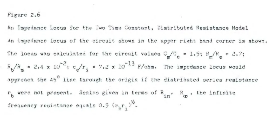
Lnly one ot~er equivalent circuit ~ith the minimum number

of ciLcuit elements is ~s~d h~re (s~e Fig. 2.7 for the circuit

and the 1dentification of varlables). The admittance vf this

Figures 2.7,

2

.

8

.

2.9

E"~v;v~l e.v. t

'rhree Different bien miaian:aat Put•t•n=e Circuits

The equations for these c1rcuits are given in the

text. The symbols in the figure identify the

!"ig. 2.7

----.-- c,

Fig. 2.8

Fig.

2

.9

r't

[image:45.620.88.538.34.781.2]

~t)

--v"'"r

+

-v~r..,.,c~

r;

f3

+~+I

r:~

I

""'v~

_~

+ r.,.]-..+

_{r ..}

,,;'-

r~

c-.. ( ~~"

(21)

+"} \)

rc

₊

:~i

[1

+

r..,J~-+

""l> ....

r ... c ... (

~r

r~ ~~

where

It is useful to ~ive the circuit parameters of the model

shown in fi~. 2.7 in terms of the circuit para~eters of the model shown in fir,. 2.6. The solution to this problem is not

unique since the d.c. p,th across the circuit may be made to

shunt either the larger oc smaller capacitance. The

~athematical re~son for this ambiguity is discussed in Appendix 1

This ambiguity does not occur in circuits where the infinite

frequency resistance is all located in one circuit element. The

values of the circuit elements in a model like th~t shown in

Fig. 2.6 are thus well determined.

The equivalence relations are

r"l.

=

c~--I-t

(H.,.-

H,)

rb

rb

l-+

.~

(

1-1

~-

11 , )

r-b

H. (

H,.-

H.)

o\,

Gf~[H, H~-

H,

(<.(,+<ll~ +~.c4;)

~

- [H.

H~-

1-t,

<..~

...

~.:'I

+

i·

~,.]

42

wnere

13

r~

c

~ -t-

r

'rl\

c

W\ +

r

)IYt

c

e

A

==

r""'

r~

cW\

c~

---D

~

,fD-;).-'iEF

'lF

D

(23)

fne other set of equiv~lcnce re~ations (for the shunt on

t~~ 0th~r capHClta~ce) can be founJ simply hy interchanging ~

₂

:1nd H

The t~o c1rcuits with more than the minimum number of

circuit elements which are of interest are shown in Fig.

2.8

~nd rig. 2.9. In.each C3se one of the resistive shunts on the

capacitance is redundant. The equations relating the circuit

values of the model shown in Fig.

2

.8

with those of the model

in rig.

2.7

are

r(l

Ce..

.

rm

-

-K

.

4-

(t-a..)

J"

1< D,

a...."J+L

L

?..

-( Cl.J

+

L)

.'Jith

t\

=

J=

L

=-l-1 (

D,- N,) (

D,-

N,.)

D, (D,

-~)

H

N,

N~

D,

D~

H

(Q,.-

tv,)(

9,..

-N,)

t>~

\O:l-

Q)

- B

~

-J

Bl.-'-#A

.

G

=

c,

c.']..

r, r::l

Yl

.

B

=

~

c,

+

r~c.l.

+

c,

(r~-+

v-

3)

Finally, the value of r (which must be known independently)

ce

f '

can b~ ~sed· to determine the parameter a (used in equations

(24) )

l -

a..

~K rce(Krc.e.+~)

). rc.~ J

\(

J-..J

These equations are ambiguous in that the symmetry of the circuit

shown in Fig.

2

.8

makes the two parallel branches.

indisting-uishable.

'rhe circuit values of the model shown in Fig.

2.9

can

easily be derived from those shown in Fig. 2.6 since both rb

and em are unchanged by the presence of r₂• That is,

Physically, this is reasonable since the high frequency behaviour

of either circuit is unaffected by the other circuit elements.

fhe equations giving the other values are

r3 (13/r..,JI

~

-

_{r~+ r~(t-~)}

r.~

r""'

(25)

c,

c-.(:

r._-\-

r~(.l-/S)~~

r.

~

""

where ~ is ~iven (in terms of the independently known parameter

I -

(3

=

_ r ._.,.,.,

+

r

~

-,J

r::

+

'i

r~

r

4

4

Curve Fitting Methods·.

An attempt was ma~a to fit the observed impedance loci using the methods of Falk

&

Fatt

(1964).

Each of the approximations used there presented difficulties here. The low frequency plot was unreliable because of the presence of a very low-!requenc7 dispersion. The high frequency plot was applicable at only t.he very highest frequencies and thus was quite tinaccurate. The m~d-frequenc)' approximation to the shape of the curve waa

not applicable because of the particular parameter values of crab fibres. Finally, the strong interaction of the various parameters prevented the refinement of inaccurate values b)' aucceasiYe approximation. It was thus necessary to develop another curve fitting technique.

The principle or the technique developed vaa to choose circuit parameters so that the deviation of the theoretical curve from ~he obserYed points waa minlmized. The deviation vas defined as the sum of the squared deviations from each experimental _point. The most satisfactory fits vere found if the theoretical curve

was fitted simultaneously to the phase characteristic and the X/R plot. (The reason for this is that the phase characteristic is particular!)' sensitive to small parameter changes.) The

t [

ct~[l?~:.-l

=,

where

k is the number of experimental observations (tho number of

frequencies at which impedance measurements were taken).

i represents the ith observation, made at frequency fi.

R~~;, -~~~~·

and

P~~~

are the resistance and reactance (in kohaa)

_.

and phase (in degrees) measUred at frequency fi' respectively •

. (i) (i) (i)

R

1, -X 1, and P 1 are the resistance, reactance, and pha8e

ca ca ca

(same units aa above) calculated at frequenc1 ri, respectivel1•

ai, bi, ci are the weights assigned to the resistance, reactance,

and phase measureaents made at frequency fi' respectively.

(Absolute rather than relative deviation is minimized since the

randoa error was felt to be relatively independent of frequency)

An electronic digital computer {The London University

Atlas) waa used to compute and minimize the function defined above.

Library Routine 970, written by D.C. Cooper !tn'd D.J. McConalogue

using the method of Rosenbrock

(1961)

and McCon&logue and

Strickland

(1963),

found the miniau. reasonably quickl7, provided

none of the parameters were too near zero. The program waa

checked by using different step lengths, initial values. and

accuracies of minimization. The major diffic·ulty with thia

method is that it cannot distinguish between aysteaatic and

random errors. The choice of the weights could compensate for

this difficulty to some extent. Because relatiyel7 aaall changea

in circuit parameter values (eaJ

15

per cent) produced large

changes in the fit of the curve, it is felt that the P-rameter

values are· w•ll determiped by the impedance·aeaaurementa, to an accuracy of about fifteen per cent.

A version of tbia program, written in Extended Mercury

APi·E:~JIX l TO Ci-iAf'rER 2.

Jerivation of the Equivalent Helations.

The conventional method of finding the relations bet~een

circuit values in potentially equivalent circuits involves the

simultaneous solution of several equations, usually those

describing the infinite frequency and zero frequency behaviour of

the circuit, and those describing the time constants of response

to a step function of applied current or voltage (Starr, 19}8).

Since these equations are usually quadratic. the mathematical

difficulties in fin1ing the simultaneous solution are formidable.

Another method of developing equivalence relations is given here.

If the impedance function is regarded as kno~n, the problem

of findin~ the equivalence relations reduces to the problem of

synthesizing a network of given configuration from a known

impedance function. '£his is a problem similar to those handled

in the theory of networK synthesis and so the methods developed

in Tuttle (1958) .,.,, ~.,illemin (lij)C,Z) can be used. The basic

approach is to synthesize part of the net•..tork from the given

impedance function and then remove that part of the circuit. The

remaining circuit is synthesized one part at a time, each time

removin~ the part just synthesized. This process of synthesis and

using different standard ('canonic •·) forms for realizing

(synthesizing) each part of the circuit, almost any configuration can be built up. For example, one way of synthesizing tbe

circuit in Fig. 2.7 (not the method used below) is by first

.using the parall~l branch canonic form and then treating the

remainder as a ladder standard form. In some cases the possibility of using different methods of synthesis leads to ambiguity in

the final equivalence relations. These cases will be discussed as they arise.

·rhe first equi.valence relations derived are tbose between the networks shown in Fig. 2.6 and Fig. 2.7. The adaittance of the circuit shown in Fig. 2.6 is known. The problem is then to synthesize a network of form given in Fig.

2.7

fro. the adaittance function given in (20) •

. It is convenient to write the adaittance in terms of the complex frequencJ variable

s

s'a.

+

s

sl.

+

s

reCe

+

r..;.cM

+

r ..

Ca

r ...

r.

c ...

c.

+

I

r,r.

c,

+

r.<.~c..

+

r..-c."" ....

r"c..)

r~r.-- r~

c.

Cct

Factoring numerator 3nd denominator gives

(s

-q,) (

s

-D\"')

(27)

(S

-~,)

(s-

Ha)

where the symbols on the right hand side of the second equation

are ~efined in (2)) of the text.

This admitt'lnce is now divided by s and expanded into

partial fractions.

:5f:_

q,OSa

..!..+

( H, -q,2(H,

-~2)

f

5

_H.

_Harb

s

rb

H,

{H,-

H~)

s

_H,

(

H~-

o(,)(

H~- ~?.)

'

+

rb

H~

(HA-

H,)

s-

H;t.

~ither the second or the third t~rm can be synthesized as the

branch containing r

1, c1 (Fig. 2.7). Only one of these two

1mbiguous cases will be developed here. It is clear that the

other can be derived simply by interchanging H₁ and H

2 in all

the following·equationa. fhe form of the admittance of the

branch containing r

1 and c1 in series is

s

c.,

(29)

The equivalence celations can be found simply by examining the

behaviour of (29) and the second term of (28.) at the extremee

of frequency.

The admittance remaining when this branch ~as been synthesized

'

and removed is called Y and can be written as

y'

~

s

+

~H~- ~.)

(

w~ -~.J

ro

H;l,

lH,..

-1--1,)

s

(30)

52

sf

~

H.

H~(H,..-

HJ

\4,

H.-

H.

\tf,+4f~)+'f,

3ut this has the same form as the admittance of the second

br~nch (cons~sttn~ of r

2, r 5, and c2) in fi~.

2

.7.

The

s

+

t3 C.?,.

~gain, examination of the behaviour of these expressions at the

extremes of frequency enables the equ1valence relations to be

der1ved.

·~he equivalence relations between circuits with redundant

parameters are also required. It is straightfor~ard, using the

above techniques, to go frorn the parameter values of a

redundant circuit to those of ll non-redundant circuit. Ho~ever,

we need the relations the other way round: going from the

parameter values of a non-redundant circuit to those of a

redundant circuit, the redundant parameter assumed ~o~n from

other information. rhe difficulty here is that some, perhaps

3ll the parameter values of the circuit being synthesized depend

on the value of the redundant parameter. The synthesis of the

circuit shown in Fi~.

2.8

from the impedance of the circuit

shown in Fi~.

2

.7

is a case 1n point since all the parsmeter

values depend on the value of the redundant element r

ce

If the admit t:mce function ( 21) is writ ten in terms of

th~ complex variable s, Jivided hy s, ex~anded into partial

...

fraction~, and multiplied by ~. the result i •

l<

s

J

+

--.;...;....;;,---5-

D,

+

LS

S-

Da

( 32)

where th• symbols J, K,

o

1,

n

2 are aa defined in (24). Sinew

the circuit.we ~ish to synthesize haa two d.c. patha₁it is

necessary to split the corresponding term (the firetmrm in (32) )

into two parts.

+

a-J

+

L.S

54

·

s-o,

·

s

-

- o

·<JJ}t~

~ -·

The procedure-'ia then to syntheaiu the desired circuit, one -··

branch being equiYalent to the· first two terma

ot

(33).

th•

other to the last two terms ot

(33).

The expression& for all the

parueters will contaiu the parueter ·'a' but •a• cau. be found

by solving for

•a•

in the expresaioa tor r _ce •

~ similar procedure enables th• equivalence relations

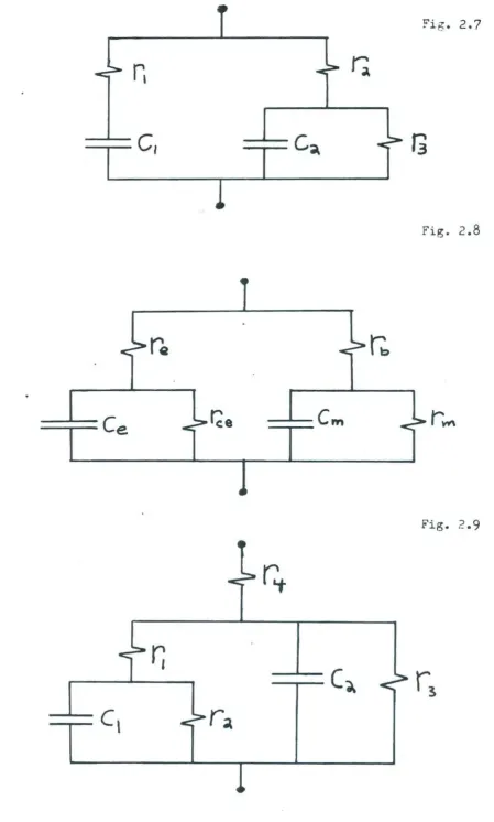
FIGURE 2.10: FLOW CHART OF COMFUTER PROGRAM FOR CURVE nTTING

DATA

INITIAL VALUES

SUBROUTINE T) • 5)

computes !unction

to be minimized

..._

._.

/

C011putes

Z

at

each frequenc1

'

Fonaa weighted dev-iation at

each

!requene1

~

Sums oyer

all frequencies

ROtrrtNE

970

Minimizes function

computed in subroutine T)

SUB~OUTINE S) s 2)

O.teraines i

r

minimua has been

found vith sufficient accurae1

I

-.

I

I

(Baa not) (Has)

[image:62.876.186.819.47.476.2]

APPDtDIX 2

ro CHAF1'ER 2.

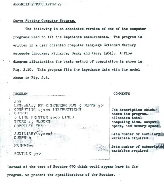
Curve Fitting Computer Prosram.

The following is an ann~tated.Yersion of one of the coaputer programs used to !it the i11pedance- measurements. Th• progr ... ia

written in a user oriented computer. language Extended "ercur1 Autocode (Brooker. Richards. Berg, and Kerr, 1961). A· flow·

~. diagrws illustrating the basic method or co11putation ia shown in Fig. 2.10. This prograa fits th•.iapedaaea data witb the model

snown in Fig.

2.6.

PROORAM COMMENTS.

I

.] 0!1

LSM32EAi·~

COMPUTING 0!JTPUT

RS EISENBER(l' RUN

S

SEPT'._.

StY

'

! 5o oo I NSTRtJC'T tONS

I

_{: Job description whic•}

.

.

_.yt

~

o LINE PRINTER 2000 LINES

STORE 2 S 8 LOCKS' · '

; C0~1PJ1t.ER.

E!'f.'l

·'"

i

.

.

..

...

I ,·( y (.' ·"j>.. \

I

AUX J·J-.. .... ~R . o~t·oo:r:;.-:··-~ :_·: : I •• OUtfpg':• q : . .

:i·

.

'· ... •'{:·'

:, .

l

...

l'tit

Ht~6cro:

·

·

. . ~

ROUT I N F:' 9 7 Cf1

. . '

.

}' ...

' names th• p.rograe.-. "·'

allocatee total.

' c011putinc time. autpu . space.- and, HJI01T spac ·

I . •

I

1 Set• nuaber of awd.Uazod

1

variable• requizecl

. ':

'"

"

..

·

.

· .

,

t

,

, .

Seta nuabu of eultaac:riiDtHII

·

-~··,i~·~···~.' ·yariable• requirecl·

I

- ··· -- J

[image:63.585.17.556.54.665.2]

'

The minimum value of the function is left-in F and the

corresponding values of the independent v~riables in

Yo, Yl ••• Y (N - 1).

'

t

•

'

'

•

I, J, _~. R, S, 1', N,

_{u ' v}

t _{F '} G , _{H '} E are used by the

routine. I, J, ~ m.<J..y be used ·for working space by either

•

•

_'

subroutine. G , H , E _{t1A1 be used} ~• working apace by

sub-routine S) •

.:lubroutine T)' computes the function of the variables Yo, ••• to

be JDinimized

Subroutine S) determine• when the miniaua is known with sufficient

accuracy. It then prints out the desired data and, by setting.

R 2 0 instruct• the routine to return to the appropriate place

in Chapter 0.

'

The program works most efficiently it all th• Y s are of the

same order of magnitude. For that reason on• or our Yariablee

•

ce/ri is written as the product X Y2. Y2 can then be chosen

t

CHAP.fER o:. A~so .9?50 C?so D?so

E?so

V~25

H?as

IJ?as G~.s;o

Y?ro

£?ro

H~so

X?

so

F"="·

02

N=J

Ui1=o

V1t=so

S)=2)

r>=s>

. READ(Kn)

I n

=

r ( r

) !<n

N F.: •·1f ... I N F.:

.! 0

6 S

I 0 ~ _{0 1} ~ • I

f'{EHLl NE.

~PTTON

RUN· ON 0/\T.o\ ~! 1').

P

P.

I NT ( I 11 ) r ₁ o

~~AD(£n)

:1=.1

~EAD(A)

RE.~D (YJ)

A=roooA

READ(Yo}

READ (Yt) READ(Ya)

Direct'ivea allocating space for

subscripted variables '

Settins variablea· required by aoutine 970

Setti~ labela required b7 Routin• 970

•

Cycle enablios:K batcbea

or

data to

be proceaaecl in ozae run

'

Identifiea each batch. of data. ill output::'-i~

Seta accuracy with which mini.wa ia co11puted

A ia Rin (kohas)

Y3 is the initial gueaa for

:a

(

kohlla) ·.

>

01)

Gonverts to ohma

Yo ia the. ~nitial. guess for C,/C

8

. Yl ia the. initial guess.

tor:

·

R-JR•

Y2· tim•• X~' ia:. the illi.tial.. gufaa

60

'

.

READ'

(Xn

·

J

P.F..J\D ( p)

P is the number of observed impedance~

P.E.J\D ( l1)

JUHP I7

, ;."'· -' ..

M

is the number of seta o! reactance weightings

----·

>>COt1PlJTES*

~

R;r:;.X;: ANDM TN I M IZES

DEVIATION~

PROM'

OBSERVED

'~

~

QXTA

..

.

.•

.

.

-

~--· - ·-- .

--

. - .

-

-5) F'=o r··-Su?routine for COIIputing function to

IJ=r oooY ,·

c=xD

r v r

DE

(uu,

AA-Ufl)

IJ=xSQRT (AA-UIJ)

K=r(r)P

V=1 XnY a ~~KtJU/Y r

I

be Dliniaaized: .the deviation. rroa the

theoretical curve

Coapute& theoretical curve·

tor

given··

set o! Y' a

>>COr1PUTES DEN0f11NATOR OF' LUr1PED E~UATIONS'

.

~ \ ,..., D=r.CVVVVYoYoYrYr+VVr,CYrYrYoYo+aVVCCYrYrYo+VVCCYrYr+aVV~~Yr

D=~VVCCYr+2VVC+VVCC+VV+CC+2C+D+r

>>cor·1POTJ:?· RM X(1 .

. .

~~G

=.VVVVCYoYoY rYr+VVCYrYrYoYo+~

VVCYrYrYo+VVf:YrYr

+~ VVC~"V

~

'l=VVC+~V~:q+~~~(l+r · I Computea the distributed coaductanc• - ...

. (j

::=r,

/D.

"'>>COMPUTES RMXB·.

'

IJ=VVVYoYt+VY"r+Wt:ro ₁ Compute& the diatributecl auaceptaac•

f1=A/D

E=Gt1. C011p1tea lu11ped parameters Y=XSQRT{i+AB /E)

'·1=XS8Ri (2Cl+a BEJ/ll)

C::=XSt:2RI(Y+r)

G=IJE/~~

X=XS8Ri(Y-r)

X:::(J X/t~

.

'

c;K~/to·oo

XK=X/rooo

.

.

.

..

>>COHPUTES THE' HE'l'(lHTED DEY I l\ T

IONS

SQUARED Hr<=xA RCTA!'! (SK ,.Xf<)

IJf<=XARCT:~/U! ( AK, BK)

HV.=r 81')H!-\/r.

'f!(=r R oUK/r.

P=F'+V!<HKHK-3 VKHK1JK+VKUI<U!<

H=CKAI<AI<-~CI<AKGK+CKGKGK+DKBKBK-aDKXKBK+Dr<XT<XK

F=F'+H

-

.

--

-

-

,

..

~EPEAT

RETURN

0 ° 0

~)L=L+r

r::L=Fn

· _with Determines 1! llillillua haa been _{sufficient accuracr} !oW1d·.

,J!Jr1P ~ L=r

'/=Ef ....

-E

fL-I)

V=xMOD

Cv/EL)

I .

r o) R=o '.Print a output

NE~·JL I NE

C .1\PT I ON:_..·~'"'~ ..• ~-' ... ·, : . . '

~fiJMBEf&

1.

0~

~

-

JiTs~~~s~~~

-

~

S1 \ PP.INT(r..) ~,o

,.

NEHLINE

C.!.PTlON

MINIMUM

SUM OP

DIF'FEReiCES -SQUARED~tiS

.. ,~

P

R I NT ( Fn ) o • 6

!'IE~JLI'NE .

CAPTL'ON-FOR

·

CM/CE::;;

·

PRINT(Yo) 3,3 CAPT.! ON

,RI-1/RE~

PRINT(YI)

3•3

CAPTI'ON

·

, CE/R

f =

PP.INT(XnYa) o,4

.

CAPi!'ON

PRH·!T(Yi) J,

,

J:

.

NEtJLINE.

I

o6s

·

,

0~.

o,.

..

S•

I ( NEHLINE:

NET·JL

INE

NEhll.INE.

K=r(r)P

toln

=

o.

S

HK

Hn=tm/e

NEHLI NE

P R I NT (

t~n )

S •

3

CAPTION

C/S

NE'oJL I.NE

CAPTION

R t~EIQHTINfl IS

PRINT(CI<)

a,o

·

NEHLINE

CAPTION

-X t~EIQHTfNq It'S PRINT(DK)

z,o

NEt·.t. INE

CAPTION

R OBS.=

PRINT {AK)

.

2•3

.

CAPTI'O~N R CALC.~:::ar·

?

RINT (4KJ' 2•

.

l

NEHLINE·

CAPTION

-X OBS=

PRINi(BK)

2."3

CAPTION

-X CALC.=

PRINT(XK)

2 1 3

NE~·!L INE

NEHLINE

Z=XRADIIJS{AK,BK)

CAPTION

/ZOBS/=

·

·

PRINT (Z) 3 3

zn~XRADIUst~K,XK)

CAPTI'On

., /ZCALC•/='"· ·'

6z

Explanation of what is being priDted. can be found in program itself

PRINT

·

(z;r)

213'

NEHLI

N

E

CAPTIOf'.l

O

AS •

.

PHASE IS

Z=XARCTAN(AK, BK)

PRINT(r8oZ/r.) 312

CAPTION

DE4REES, CALC.

P

HASE I

S

~=XARCTAN(4KtXK)

PRINT{r8oZ/CJ 3_{1 2}

CAPTION

DEClREES

.r,n:xSIN(I<£/4)

c;n=xMoo(qn)

JUf1P' 47,4n>o. ooor

NEt•JL INE

ro6s.

,

o.,

·

o •

.S•

r

47)~11=o

nEHLINE

rr

E~·1L l N E.

~!F:HLINE .

f•!E"lL INE ~EPE.~~T·

~)RETURN

I

7) K=r

K

=r(r)P

R

EAD

(l.JK)

R

E.'\0

(AK%)

R

E

.

A.D(CK)

P.

EAD(BK)

READ (DK}

RE:'\D (VK)

1.JK

=a£HK

R

EPEAt

O

=t(r)M

,JJJMP., .lF. ... O;:tn·: ·

Computes phas•

Reads in cia ta

..

Cycl• reada in at each fr•quenCJf4< '

·

•k,

th• trequencJ o:-·

Ak, R (resistanc•)

C~ the Rtweighting

Bk, X

•(reactanc•)

Dk, X ve'ighting

~~=r ( r) P

PEAD(DK)

REPEAT

NEt~ LINE

! 0 6 S 1, 0 •' 0 ,_ S e I

s

I )JUMPDO!t!N (R9 70)

~EPEJ\T

~EPEAi

F.:~ID

CLOSE

Reads in additional set of

X ~eightings, if desired

Calla in Houtine 9?0

text brackets surround the name and meaning of the number found in

the corresponding position (but without bracketa) on the print out

of a data tape shown on the next pa~e. Every end of a line iD

the print out is indicated belov vitb the sysbol~ To illustrate:

t

" correep<)nds to the first nuaaber on the second line ot the print out;.,.

A, to the second number in the second line; etc.

t

(K the nuaber of batches of data) NL

-t

( x the accuracy of the Dlinimua)

(A the value of the input resistance)

(Y}. the estimate ot the infinite frequeDCJ resistance)

(Yo the estimate ot CmfCe)

(Yl th.e eatimate of RafRe>

(YZ a t~ctor ot the estimate of c~ri)

t

(X a factor of the estimate of c~r

₁

)

(P the nwaber of observed illpedaDcea)

(M the number of batches of reactance weigbtinge) ~

(ltk the frequencJ)

· (Ak the obaened resistance)

'(Ck the weighting of the resistance)

(Bk the obaerved reactance)

(D~ th•·weighting of the obserYed.reactance)

(Vk the phase weighting) NL

-This last line is repeated once for each frequency at which

impedance ••aaurementa were made; that is, P times.

•

The entire set

ot

data is repeated (vith the exception of K ) for each batch of data.

# .., ,_,

o.'ooar· 20•72

o.s

2

r

8

r,.-r3

r.'ooo 20•'79

r

r.69 t _o.

s

r.:J68 , ao •. o9. I.. • . z •. 86 r

3··-tl;.~

...

e

o •

.as

a. 54< .. . I'J•70,'

r

·

Oe2-S

3•'r6a · '-r·9•al' I _',

1•

_,

x

r. · _..... t.:. 0•.3.5::

1• 6121 .. I 7.~89 I _{~.; S!l ..} I . oa·zs··

6.i8r.r

rs ..

67

1:

·

.!lot

.

.

•

.

I.

o.2

·

s

ro.'ot>

t3.!46.

.t 6•71. r .

o-.

.

2s

I 1•'68 t r.'o2' I _7•oS. I a. 25.

3 I •' 51' 'J•'oa I 6.87 I Oe25

3r~6a .. 7•'ra r.· S• 89 I

o.as

'46el{a-

S~97 I

.S•

_{a a} I Oe2S

68.J

r

4

.·.

1~24 I

_3•9°

I o.as

rooi.d _{3 .. 79} r· _l-124 I· _o.as

I _.1)~8- _{3 .. 28· I a-. 68: ' r Oe25}

f ' · I

ars.-f4 a.Wa r a. r6~·: r Oe3S

.3.r6e!a :h S.;'J ..

r.

'.

t:t•

'

9df

•l

t .,~o

as

• ,. • . . -r

...

.

;t~tt~% , ....

_·.

, ..

,

~ ~~

r Ill

.46~

1

2 2 e

1

IO'- r · r.•ts~··

·

r

o.25

6:9 ... ) 1

_.,

_.

_r.?

r~

r

·

,

r •. a.r·'

r

·

r.oz

r

r o .. a4 r

t

r

o.

7·1 t

r 6.S8 t t o.s6 r

--~~

1!

-

t

r;. _o.as

o.:a

·

s

o-. aS.

o-,as

o.as

o.

'as

o. ~s

Chapter }.

METHODS.

Material and Apparatus.

The preparation used in these experiments was the flexor

of the carpopodite of the _first walking leg of Fortunua depurator

and Carcinus maenas bathed in crab Ringer solution (Pantin, 1934;

Fatt

&

Katz, 1953a). 'fhe flexor muscle was exposed by removing

the opposite part of the shell, together with the extensor muscle

and limb nerves. The ahell beneath the flexor was removed to

improve visibility and the muscle viewed in transmitted lilbt.

Surface fibres in the middl• half or the muscle and on the wide

aide of the apodeme wer• used for these experiments.

Micropipettes with reaiatancea or about

4

segohma (measUred

when dipping into crab Ringer) were inaerteo into fibres on the

exposed surface ot the muscle under aicroscopic observation.

Microelectrodea used to apply currentto the euacle fibre were

filled with 2M sodiu. citrate (pH _...

6)

since these passed greater

currents than the microelectrodea, filled with 3~ KCl, which

were used to record potential. Measurements or distance were made

-with the eyepiece graticule of the microscope.

Fi~e 3.1 shows a schematic drawing of the experimental set-up. rhe cathode followers (shown in Fig. 3.1 aa triangles

Figure 3.1

· Diagram

ot

the

Set-up used· tor

tlii

Measureaent

_

bf

lmPeclanee vith Miei-oeleetrodee

~ .

The triaDgles 8urrounding the

'1

In most experiments · ·cathode

.

amplifier. Identif1eati6n of

~

leiiera "CF'' reprfsent

~athode toll~e~s.

• ' I I f" ,

follower waa uaea

bet~een

,

-

...

ald

t~e c~rrent

"· lion

I ... I .

symbols and further discileaion round ill text.

[image:76.875.217.801.202.378.2]

Shield

~ 1 1 Voltage

-Current

mol~;;

""liP WS

d

I

!_

__

J,e>-::-:<'Z''>', , ...

_{_...._._..._}

_...

_

z

_

,

_{__}

~~_.,_

__

p ..

cc,« '' 'S '"

« '"' \\ ''

'5" ''

''!\

I

Potentiometer

Pelti~

Coolins

El~~e~~

R

IDOD

vertical) amplifier

Current horizontal uplifier

c

.a.T.

·

0

[image:77.890.99.873.85.566.2]

surroundins th4r letters "CF") used. for di!fereistial. voltage

measurements were arranged so that a ssall amount of attenuation

could be applied to one or the other to improve the rejection

ratio of the· recordin~ system. The potentio.eter waa a d.c.

voltage source used to offset the resting potential of the muscle

fibre and waa repl&ced with a calibrator to measure the gain of

the voltage and current recording chaanela. The potentioaeter

w3a enclosed in a screening box driven b7 a separate cathode

follower in order to reduce the capacitance to earth, which would

f

otherwise significantly ahunt the. current eonitoring resistance

at hi~ frequenc7. The calibrator could. not b• u.aecl to oftaet

--e..

ff..c.

c.

t.

~

th• resting potential si~ce ita~capacitance to-eart~ waa quite

•

large. eve~ when. enclos&d iaA driven box.

Because· or the larg• teaperature co-efficient of ••brane

reaiatance.. in crab IIUacle (Fatt & Katz •.

l953a)

t•pel"ature had.

to be accuratel1 controlled. A aelliconductor. conatant. t~ature

device (Copeland. 1961, 1962) waa. wsecl to maintain, th• auacle•,

o· · o

at • conatant te~~peratura

<.:t

0.1 C)' arouncl 5. C. Thia dericW.

introchlc••· a larg& capacitance. to earth· sinc8' the coolins eleHata

in the circuit were esaentiallJ earthed. and wer~ cloe• to the

bathing solution. This capacitance waa reduced. b7 placing an inaulatect. ~

ehield between the coolin~ eletaenta ancl the bath and driviDs it.