Abstract—After bugs are detected, it is crucial to identify their severity levels to avoid any effects that may obstruct to the whole system. Unfortunately, only a small number of defected are reported along with their severity level (labeled data), while most of them do not have it (unlabeled data). All prior works employed tradition-al supervised learning techniques that just replied on this small amount of labeled data. Furthermore, they ignored a bias that is caused by an imbalanced issue since some severity levels may have defects much larger than others. In this paper, we aim to improve prediction accuracy of the defect severity categorization by proposing a novel algorithm called “OS-YATSI.” It employs semi-supervised learning to fully utilize all data and applies an oversampling strategy to tackle the imbalanced issue. The experiment was conducted on three public benchmarks of Java software. The results showed that our algorithm significantly outperformed all baseline classifiers, i.e., Decision Tree, Random Forest, Naïve Bayes, k-NN and SVM, on all data sets at an average of 28.79% improvement in terms of macro F1.
Index Terms—software defect severity; defect severity categorization; semi-supervised learning; imbalanced issue
I. INTRODUCTION
OFTWARE defect is any flaw or imperfection in a software product or process. It is also referred to as a fault, bug, and error. Different defects have different impacts on the software. Some of them may only slow down the process, while others may be a cause of failures to the whole system. Therefore, it is important to categorize a severity level of each defect, which can help developers to prioritize the defects and prevent any serious damages to the whole system.
There were many attempts to automatically classify defect severity. Almost all of them require a user feedback called “bug report” as an input. SEVERIS [1] is a software severity assessment system that utilize a textual description from reported issues. [2-4] applied classical data mining techniques to predict a severity level from user feedbacks. [5, 6] employed a text mining algorithm along with a mechanism to select important keywords from bug reports. Unfortunately, these works heavily replied on the bug description, which means that users must already encounter errors and serious damages may already occur. Thus, it is better to capture all defects along with their severity level directly from a software metrics during the software
Manuscript received December 8, 2015; revised January 6, 2016. T. Choeikiwong and P. Vateekul are with the Department of Computer Engineering, Faculty of Engineering, Chulalongkorn University, Bangkok, Thailand e-mail: [email protected], [email protected]
production stage.
At the production stage, the number of reported defects is usually small. Moreover, only a small number of defects are described along with their severity level (known as “labeled data”), while most of them do not have it (denoted as “unlabeled data”). For example, the Eclipse PDE UI project [7] has 209 defective modules composing of 59 defects (28.23%) and 150 defects (71.77%) of known and unknown severity levels, respectively. Furthermore, 46 defects (77.97%) of defects with severity levels are defined as “moderate effects (Level 2)” out of 3 levels. This circumstance is referred as “imbalanced issue,” which the result tend to classify most defects belong to the majority level and tremendously drop prediction performance. Therefore, it is not a good idea to employ a supervised learning model that solely relies on just label data without concerning of imbalanced data.
Semi-supervised learning is a technique that tries to improve a prediction accuracy by using both labeled data and unlabeled data for training. In a literature survey [8], traditional semi-supervised learning algorithms are divided into four main groups including Self-training, Co-training, Density-based, and Graph-based methods. The success of semi-supervised learning depends on underlying assumptions in each model. The self-training approach is the most popular semi-supervised learning technique, since it is simple and can be easily applied to almost all existing classifiers.
In this paper, we present a novel defect severity categorization called “OS-YATSI,” that combines between YATSI [9], a self-training classifier, and SMOTE [10], an oversampling strategy. It improves a prediction accuracy by utilizing unlabeled data, while correcting imbalanced issue all together. The experiment was conducted based on three public benchmarks [7] and, then, the result was compared to the original YATSI and several supervised learning techniques: Decision Tree (DT), Random Forest (RF), Naïve Bayes (NB), k-NN and SVM.
The rest of paper is organized as follows. Section II presents an overview of the related work. Section III describes the proposed method in details. Section IV shows the experimental results. Finally, this paper is concluded in Section V.
Improve Accuracy of Defect Severity
Categorization Using Semi-Supervised
Approach on Imbalanced Data Sets
Teerawit Choeikiwong and Peerapon Vateekul
II. RELATED WORK
A. Software Metrics
In the field of software engineering, software metrics play an important role in describing the software. They are also known as “code features”. It is common to use them to control the software quality and to predict possible errors along with their severity levels. In this work, the code features of the experimental data sets are based on Chidamber and Kemerer (CK) metrics and Object-Oriented (OO) metrics [11] as shown details in Table I.
B. Related Work in Defect Severity Classification
There were many trials that applied text mining and machine learning techniques in the area of software defect severity prediction. In 2008, [1] proposed a method named SEVERIS (SEVERITY Issue assessment) based on RIPPER, a rule learning algorithm, on the textual descriptions from issue reports. It was experimented on five nameless PITS projects consisting of 775 issue reports with about 79,000 words. By considering the top 100 terms, the F1-result was in the range of 65% - 98% only for cases with more than 30 bug reports.
In 2010, [2] applied Naïve Bayes algorithm to predict severity levels based on textual description of defect reports. There was an investigation on the three open-source projects from Bugzilla. The result showed that it achieved a promising performance in terms of precision and recall. In addition, this study has been extended to compare with four classifiers [3]. The experiment concluded that Multinomial Naïve Bayes does not only show the highest accuracy, but it is also faster and requires a smaller training set than other classifiers. Another study, [4] compared six classical classifiers, but there was no conclusion on the winner method. In 2012, [5] aimed to improve an accuracy of severity prediction by investigating three feature selection schemes: Information Gain (IG), Chi-Square (CHI), and Correlation Coefficient (CC), on Naïve Bayes. The experiment was conducted on four open-source components from Eclipse and Mozilla. In 2014, [6] demonstrated that bi-grams and Chi-Square feature selection can help to enhance an accuracy of
the severity categorization task.
As mentioned above, none of prior works have ever applied semi-supervised learning techniques to improve a prediction accuracy by utilizing unlabeled data. Moreover, all of them ignored an imbalanced issue resulting in a prohibited accuracy.
C. Strategies to Handle Imbalanced Data Sets
To tackle imbalanced issue, a sampling technique has received the most attention and is reported to be the best strategy. These techniques are mainly dividing into two approaches as follows.
Undersampling approach tries to balance between two classes by removing examples in the majority class until the desired class ratio has been achieved. Unfortunately, it is not suitable for small training data and it cannot guarantee to keep all important examples.
Oversampling approach is an opposite of the undersampling strategy. It helps to improve a balance between classes by replicating examples in the minority class; thus, it is suitable when there is a scarcity issue in the training data. However, a duplication of minority data can cause an overfitting issue, so it is common to generate new minority examples instead. SMOTE (Synthetic Minority Over-sampling TEchnique) is chosen to use in this work and its details will be shown in Section III.
D. Performance Measures
In the domain of binary classification problem, it is necessary to construct a confusion matrix, which comprises of 4 based quantities as shown in Table II. These four values are used to compute Precision (Pr) and Recall (Re) and Fβ
-measure introduced by [12] are shown in Table III.
As mentioned earlier, there are two ways to combine those common measures [13]: macro-averaging and micro-averaging as shown in Table IV. Macro-micro-averaging gives an equal weight to each class, whereas micro-averaging gives an equal weights to each class based on a number of examples. In an imbalanced situation, it is appropriate to use macro-averaging over micro-macro-averaging in order to avoid a dominance of majority classes.
TABLE I
CLASS LEVEL SOFTWARE METRICS
Symbol Description
Chidamber and Kemerer Metrics WMC Weight Method per Class DIT Depth of Inheritance Tree RFC Response for a class NOC Number of Children
CBO Coupling Between Object classes LCOM Lack of Cohesion in Methods
Object-Oriented Metrics
NOA Number of attributes NOPA Number of public attributes NOPM Number of public methods NOPRA Number of private attributes NOPRM Number of private methods NOMI Number of methods inherited NOAI Number of attributes inherited LOC Number of lines of code NOM Number of methods
FanIn Number of other classes that reference the class FanOut Number of other classes referenced by the class
TABLE II A CONFUSION MATRIX
Predicted Positive Predicted Negative
Actual Positive TP FN
Actual Negative FP TN
TABLE III
PREDICTION PERFORMANCE METRICS
Metrics Definition Formula
Precision
a proportion of examples predicted as defective against all of the predicted
defective TP FN
TP
Recall
a proportion of examples correctly predicted as defective against all of the
actually defective TP FN
TP
Fβ -measure
a weighted harmonic mean of precision
and recall Pr Re
(Pr)(Re) 2
III. APROPOSED METHOD
In this section, we illustrate details of “OS-YATSI,” our proposed defect severity classification. Fig. 1 shows a process diagram of our method consisting of three main modules: (i) Oversampling, (ii) Semi-supervised Learning, and (iii) Unlabeled Selection Criteria.
1) Oversampling
This module aims to alleviate a bias from the majority severity level. SMOTE, an oversampling strategy, is chosen since the number of defects is scarce. It generates synthetic examples from the minority class. First, i-th minority example (𝑥𝑖) is randomly selected along with its nearest
neighbor in the minority class (𝑥̂𝑖). Second, a new synthetic
example (𝑥𝑛𝑒𝑤) is calculated following the equation below,
where 𝑟 is a random number between 0 and 1. Finally, this process repeats until all minority examples are processed and generated their synthetic examples.
𝑥𝑛𝑒𝑤= 𝑥𝑖+ (𝑥̂𝑖− 𝑥)(𝑟) (1)
2) Semi-Supervised Learning
In the bug repositories, some defects have severity levels reported (labeled data), while most of them do not have it (unlabeled data). This process focuses on utilizing unlabeled defects by employing a semi-supervised learning classifier called “Yet Another Two Stage Idea (YATSI),” which consists of two stages.
In the first stage, an initial classifier is constructed only from the oversampling labeled data from Section 3.1. Then, it is used to predict a severity level for each unlabeled data. The output unlabeled data with predicted severity are called “pre-labeled data.”
In the second stage, the nearest neighbor algorithm is applied on a combined data set between the labeled and pre-labeled data to determine a predicted severity level of the unlabeled data. A weighting strategy is referred to as the amount of trust. It is applied to a distance during the process of finding a neighbor. As a default value, the weight of the labeled data is set to 1, while the weight of the unlabeled data is equal to F × (N/M), where N and M denote the number of labeled and unlabeled data, consecutively, and F denotes a user-defined parameter between 0 and 1 showing a trust on the unlabeled data.
Finally, all unlabeled data are assign their actual severity level. The k-nearest neighbor is employed. It predicts the level that gives the largest total weighting score.
3) Unlabeled Selection Criteria (USC)
After Section 3.2, all unlabeled defects are already annotated and have their severity level, so an enhanced training data can be created by combining between the labeled and unlabeled data.
For the labeled data, we choose to use the oversampling data from Section 3.1 to avoid the imbalanced issue. For the unlabeled data, the traditional semi-supervised classifier usually uses all of them without concerning the imbalanced issue. However, the preliminary experiment showed that there is still an imbalanced issue in the unlabeled data.
Therefore, this module called “USC” is proposed as a criteria to select examples in the unlabeled data set to include in the training data set while maintaining the balance of data for each severity level as summarized below:
1. Find the class with the smallest amount of example (also called minority class) and add all examples in that class to the training data.
2. Select examples for each severity level equally to those in the minority class by their prediction score from module 2 (Semi-supervised Learning)
[image:3.595.44.293.299.338.2]The pseudo code for OS-YATSI is shown below. Fig. 1. A process diagram of the proposed method
1. Oversampling 2. Semi-supervised Learning
3. Unlabeled Selection Criteria
[image:3.595.305.559.359.815.2](USC)
TABLE IV
Macro-averaging and micro-averaging of precision, recall, and Fβ, i is a class index.
Metrics Macro-averaging Micro-averaging
Precision
Recall
Fβ
-measure
1 1
i L i
MaPr Pr
L
11( )
L i i L
i i
i
tp MiPr
tp fp
1
1
i L
i
MaRe Re
L
11( )
L i i L
i i
i
tp MiRe
tp fn
, 1 1
i L i
MaF F
L
2
2
( 1) MiPr MiRe MiF
MiPr MiRe
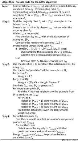
Algorithm Pseudo code for OS-YATSI algorithm
Input: A set of label 𝐿 = {𝑙1, 𝑙2, 𝑙3}, classifier 𝐶, labeled data 𝐷𝑙,
unlabeled data 𝐷𝑢, oversampling ratio 𝑅𝑜𝑠,
oversampling labeled data 𝐷𝑜𝑠𝑙, number of nearest
neighbors 𝐾, 𝑁 = |𝐷𝑜𝑠𝑙|, 𝑀 = |𝐷𝑢|, unlabeled data
example 𝑑𝑢
Step1: Find the majority class 𝑙𝑀 with |𝐷𝑀| examples in the
labeled data 𝐷𝑙
Create a set of minority classes 𝐿𝑚 that excludes the
majority class 𝑙𝑀
While(𝐿𝑚 is not empty)
Find the class 𝑙𝑀in 𝐿𝑚 with the least number of
examples, |𝐷𝑚|
Compute the number of examples |𝐷𝑚′ | if
oversampling using SMOTE with 𝑅𝑜𝑠
If ( Diff(|𝐷𝑚′|, |𝐷𝑀|) < Diff(|𝐷𝑚|, |𝐷𝑀|)) Then
Oversampling the class using SMOTE with 𝑅𝑜𝑠
Add the new oversampled example into 𝐷𝑜𝑠𝑙
Else
Remove class 𝑙𝑀 from a set of classes 𝐿𝑚
Step2: Use the classifier 𝐶 to construct the initial model 𝑀1 by
using 𝐷𝑜𝑠𝑙
Use the 𝑀1 to “pre-label” all the examples of 𝐷𝑢
For(i=1 to 𝑁) Weight = 1.0 For(j=1 to 𝑀)
Weight = (𝑁/𝑀) ∗ 𝑊𝑒𝑖𝑔ℎ𝑡𝐹𝑎𝑐𝑡𝑜𝑟 𝐹 Combine 𝐷𝑜𝑠𝑙 and 𝐷𝑢to generate 𝐷
For every example in 𝐷𝑢
Find the 𝐾-nearest neighbors to the example from
𝐷 to produce set 𝐷𝑘𝑁𝑁
For i=1 to K
If(class of 𝐷𝑘𝑁𝑁 = 1) sum weight1 of 𝐷𝑘𝑁𝑁
If(class of 𝐷𝑘𝑁𝑁 = 2) sum weight2 of 𝐷𝑘𝑁𝑁
If(class of 𝐷𝑘𝑁𝑁 = 3) sum weight 3of 𝐷𝑘𝑁𝑁
Predict the actual class with the largest total weighting score
Step3: For unlabeled data 𝐷𝑢
Find the class with smallest amount of example and produce set 𝐶𝑠𝑚𝑎𝑙𝑙
For another class
Select examples equally to 𝐶𝑠𝑚𝑎𝑙𝑙 with their
prediction score and produce set 𝐶𝑏𝑎𝑙𝑎𝑛𝑐𝑒
IV. EXPERIMENTS AND RESULTS
A. Data Sets
We use the public benchmark presented in [7]. The data set provides metrics that describes software artifacts from five open-source software systems. We selected three software system since there are enough training examples to predict the defect severity. The severity statistics is shown in Table V. From the statistics, it has shown that the data set suffers from the scarcity and imbalanced issue. An average percentage of the severity class is 35.77%, and the minimum percentage is only 1.22% of severity level 3 in Mylyn.
B. Experimental Setup
In this section, shows how to conduct the experiments in this paper. It is important to perform data preprocessing steps including numeric-to-nominal conversion and data scaling. Then, we compare the prediction performance among different methods as the following steps. Note that all experiments are based on 3-fold cross validation.
Step1: find the baseline method which is the winner of the standard classifiers: Decision Tree (DT), Random Forest (RF), Naïve Bayes (NB), k-NN and SVM
Step2: find the best setting for OS-YATSI whether or not USC is necessary
Step3: compare OS-YATSI (Step2) to the YATSI and baselines (Step1) along with a significance test using unpaired t-test at a confidence level of 95%
C. Results and Discussion
The comparison of the baseline methods.In order to get the baseline methods for each data set, five classifiers: Decision Tree (DT), Random Forest (RF), k-Nearest Neighbor (k-NN), Naïve Bayes (NB), and Support Vector Machine (SVM) were tested and compared in terms of Pr, Re, and F1 (Table VI). For each row in the table, the boldface method is a winner on that data set. From the result, k-NN showed the best performance in terms of macro and micro-average on Mylyn, while the remaining data has been effective from various methods. For F1-measure, we selected the winner as a baseline methods in both macro and micro-average as summarized in Table VII.
The comparison of OS-YATSI with and without USC. In this section, we aim to give the best setting for OS-YATSI by testing whether or not the Unlabeled Selection Criteria can deal with the imbalanced issue and improve the prediction performance. The results in Table VIII demonstrate that the OS-YATSI with USC performs better than without USC all data sets. The results imply that all the unlabeled data is not always optimize the performance prediction. Moreover, the efficiency may be reduced as well.
The comparison of OS-YATSI, YATSI and baseline methods. In this section, we compare OS-YATSI to the baseline methods which are obtain from the first experiment as shown in Table VI. Furthermore, we also compare to the original YATSI as well. In Table IX shows a comparison in terms of Pr, Re, and F1 both macro and micro-average. All of the measures give the same pattern that OS-YATSI outperforms the other method in all most all of the data sets. In macro-average, OS-YATSI significantly won 3, 1, and 2 on Pr, Re, and F1, respectively. On average, macro F1 of OS-YATSI outperforms that of the baselines for 28.79%, especially for the PDE UI data set showing 49.31% improvement. Consequently, this demonstrates that it is effective to apply OS-YATSI as a main mechanism to categorize defect severity of software modules.
TABLE V
SEVERITY STATISTICS FOR EACH DATA SET
Data #modules Severity(Sev.) level %Sev.
lv. 1 lv. 2 lv. 3 N/A
Eclipse JDT Core 206 12 19 10 165 19.90 Eclipse PDE UI 209 7 46 6 150 28.23
Mylyn 245 127 15 3 100 59.18
Average 220 48.67 26.67 6.33 138.33 35.77
TABLE VI
COMPARISON PREDICTION PERFORMANCE MEASURES OF THE CLASSICAL CLASSIFIERS
Precision
Data DT RF k-NN NB SVM
Macro Micro Macro Micro Macro Micro Macro Micro Macro Micro JDT Core 0.330 0.445 0.293 0.366 0.302 0.317 0.419 0.344 0.186 0.440 PDE UI 0.263 0.630 0.257 0.746 0.261 0.679 0.255 0.546 0.258 0.763 Mylyn 0.291 0.855 0.321 0.855 0.361 0.758 0.318 0.745 0.292 0.876 Avg. 0.295 0.643 0.202 0.656 0.308 0.585 0.331 0.545 0.245 0.693 SD 0.034 0.205 0.153 0.257 0.050 0.235 0.083 0.201 0.054 0.226
Recall
Data DT RF k-NN NB SVM
Macro Micro Macro Micro Macro Micro Macro Micro Macro Micro JDT Core 0.393 0.445 0.291 0.366 0.272 0.317 0.356 0.344 0.329 0.440 PDE UI 0.318 0.630 0.319 0.746 0.290 0.679 0.233 0.546 0.326 0.763
Mylyn 0.325 0.855 0.345 0.855 0.347 0.758 0.323 0.745 0.333 0.876 Avg. 0.345 0.643 0.318 0.656 0.303 0.585 0.304 0.545 0.329 0.693 SD 0.041 0.205 0.027 0.257 0.039 0.235 0.064 0.201 0.004 0.226
F1-measure
Data DT RF k-NN NB SVM
Macro Micro Macro Micro Macro Micro Macro Micro Macro Micro JDT Core 0.349 0.445 0.255 0.366 0.280 0.317 0.350 0.344 0.230 0.440 PDE UI 0.275 0.630 0.285 0.746 0.275 0.679 0.241 0.546 0.288 0.763
Mylyn 0.307 0.855 0.332 0.855 0.351 0.758 0.315 0.745 0.311 0.876 Avg. 0.310 0.643 0.291 0.656 0.302 0.585 0.302 0.545 0.276 0.693 SD 0.037 0.205 0.039 0.257 0.043 0.235 0.056 0.201 0.042 0.226
V. CONCLUSION
Although it is an important task to classify software defect severity levels, an accuracy of existing techniques is still limited due to two major issues. First, it is a scarcity of defects that have severity levels labeled, while the remaining are left unlabeled. Second, defects of some severity levels outnumber the others causing an imbalanced issue.
In this paper, an algorithm called “OS-YATSI” is proposed to tackle these issues by introducing a semi-supervised learning to solve the scarcity problem and oversampling defects in the minority class to alleviate the imbalanced issue. There are three modules in the system: (i) Oversampling, (ii) Semi-Supervised Learning, and (iii) Unlabeled Selection Criteria. First, we balance the number of defects for each severity level using an oversampling technique called SMOTE, so the initial classifier will not be biased by any majority severity levels. Second, the defects without severity
levels (unlabeled data) are identified using a semi-supervised technique called YATSI. Finally, these unlabeled defects with predicted class are selected equally for each severity level by their prediction score. Then, they are combined with the oversampled labeled defects from the first process to build a final classifier.
In the experiment, OS-YATSI was compared to five conventional classifiers: Decision Tree, Random Forest, Naïve Bayes, k-NN, and SVM, on three Java projects. The results revealed that our approach significantly surpassed all baselines on all data sets in terms of macro F1. In the future, we plan to propose a measure to rank defects within the same severity level.
REFERENCES
[1] T. Menzies and A. Marcus, "Automated severity assessment of software defect reports," in Software Maintenance, 2008. ICSM 2008. IEEE International Conference on, 2008, pp. 346-355. [2] A. Lamkanfi, S. Demeyer, E. Giger, and B. Goethals,
"Predicting the severity of a reported bug," in Mining Software Repositories (MSR), 2010 7th IEEE Working Conference on, 2010, pp. 1-10.
[3] A. Lamkanfi, S. Demeyer, Q. D. Soetens, and T. Verdonck, "Comparing Mining Algorithms for Predicting the Severity of a Reported Bug," in Software Maintenance and Reengineering (CSMR), 2011 15th European Conference on, 2011, pp. 249-258.
[4] K. K. Chaturvedi and V. B. Singh, "Determining Bug severity using machine learning techniques," in Software Engineering (CONSEG), 2012 CSI Sixth International Conference on, 2012, pp. 1-6.
[5] Y. Cheng-Zen, H. Chun-Chi, K. Wei-Chen, and C. Ing-Xiang, "An Empirical Study on Improving Severity Prediction of Defect Reports Using Feature Selection," in Software Engineering Conference (APSEC), 2012 19th Asia-Pacific, 2012, pp. 240-249.
[6] N. K. Singha Roy and B. Rossi, "Towards an Improvement of Bug Severity Classification," in Software Engineering and Advanced Applications (SEAA), 2014 40th EUROMICRO Conference on, 2014, pp. 269-276.
[7] M. D'Ambros, M. Lanza, and R. Robbes, "An extensive comparison of bug prediction approaches," in Mining Software Repositories (MSR), 2010 7th IEEE Working Conference on, 2010, pp. 31-41.
[8] X. Zhu, "SemiSupervised classification learning survey," Computer Sciences TR 1530 , University of Wisconsin-Madison 1530, Dec. 2005 2005.
[9] K. Driessens, P. Reutemann, B. Pfahringer, and C. Leschi, "Using Weighted Nearest Neighbor to Benefit from Unlabeled Data," in Advances in Knowledge Discovery and Data Mining. vol. 3918, W.-K. Ng, M. Kitsuregawa, J. Li, and K. Chang, Eds., ed: Springer Berlin Heidelberg, 2006, pp. 60-69. [10]N. V. Chawla, K. W. Bowyer, L. O. Hall, and W. P.
Kegelmeyer, "SMOTE: synthetic minority over-sampling technique," J. Artif. Int. Res., vol. 16, pp. 321-357, 2002. [11]S. R. Chidamber and C. F. Kemerer, "A metrics suite for object
oriented design," Software Engineering, IEEE Transactions on, vol. 20, pp. 476-493, 1994.
[12]C. J. V. Rijsbergen, Information Retrieval, 2 ed. London: Butterworths, 1979.
[13]Y. Yang, "An Evaluation of Statistical Approaches to Text Categorization," Inf. Retr., vol. 1, pp. 69-90, 1999.
TABLE VII
THE WINNER OF THE BASELINE METHOD FOR EACH DATA SET IN TERMS OF F1-MEASURE
Data Winner F1
Macro Micro JDT Core NB 0.350 0.344 PDE UI SVM 0.288 0.763 Mylyn k-NN 0.351 0.758
Avg. - 0.330 0.622
SD - 0.036 0.240
TABLE VIII
A COMPARISON OF OS-YATSI BETWEEN WITH AND WITHOUT USC IN TERMS OF F1-MEASURE
Data With USC Without USC
Macro Micro Macro Micro JDT Core 0.484 0.513 0.459 0.491
PDE UI 0.430 0.746 0.290 0.629 Mylyn 0.361 0.807 0.349 0.800 Avg. 0.425 0.689 0.366 0.640
SD 0.062 0.155 0.086 0.155
TABLE IX
COMPARISON PREDICTION PERFORMANCE MEASURES OF OS-YATSI, YATSI, AND BASELINE METHOD.
THE BOLDFACE METHOD IS A WINNER ON THAT DATASET
Precision
Data Baseline YATSI OS-YATSI
Macro Micro Macro Micro Macro Micro JDT Core 0.419 0.344 0.406 0.410 0.514* 0.513**
PDE UI 0.263 0.630 0.297 0.730 0.436** 0.746
Mylyn 0.361 0.758 0.329 0.759 0.426* 0.807*
Avg. 0.348 0.577 0.344 0.633 0.459 0.689 SD 0.079 0.212 0.056 0.194 0.048 0.155
Recall
Data Baseline YATSI OS-YATSI
Macro Micro Macro Micro Macro Micro JDT Core 0.393 0.445 0.390 0.410 0.499 0.513*
PDE UI 0.326 0.763 0.360 0.730 0.464* 0.746 Mylyn 0.347 0.758 0.348 0.759 0.366 0.807*
Avg. 0.355 0.655 0.366 0.633 0.443 0.689 SD 0.034 0.182 0.022 0.194 0.069 0.155
F1-measure
Data Baseline YATSI OS-YATSI
Macro Micro Macro Micro Macro Micro JDT Core 0.350 0.344 0.381 0.410 0.484* 0.513**
PDE UI 0.288 0.763 0.324 0.730 0.430* 0.746 Mylyn 0.351 0.758 0.330 0.759 0.361 0.807*