warwick.ac.uk/lib-publications
A Thesis Submitted for the Degree of PhD at the University of Warwick
Permanent WRAP URL:
http://wrap.warwick.ac.uk/108907
Copyright and reuse:
This thesis is made available online and is protected by original copyright.
Please scroll down to view the document itself.
Please refer to the repository record for this item for information to help you to cite it.
Our policy information is available from the repository home page.
T H E B R IT ISH LIBRARY
R R IT IC L IT U C C IC C C D V R -C J ^
-M ulti-O bjective Scheduling and Control
of a N onlinear A utom otive Powertrain
T I T L E ...
A U T H O R ... K. S. Garbett ...
D E G R E E ...
A W A R D I N G B O D Y University of Warwick
...
September 1991
T H E S IS
N U M B E R ...
T H I S T H E S I S H A S B E E N M I C R O F I L M E D E X A C T L Y A S R E C E I V E D
T h e quality o f this re p ro d u ctio n is dependent u p o n the quality o f the original thesis su bm itte d f o r m icrofilming. Eve ry effort has been m ade to e n su re the highest quality of re p ro d u ctio n .
S o m e pages m ay have indistinct print, especially if the original papers w e re p o o rly p ro d u ce d o r if the aw a rdin g b o d y sent an in fe rio r copy.
If pages are missing, please c on tact the aw a rdin g b o d y w h ich granted the degree.
P re vio u sly cop yrigh te d m aterials (journal articles, p u blished texts, etc.) are n o t film ed.
T h i s c o p y o f t h e t h e s i s h a s b e e n s u p p lie d o n c o n d i t io n t h a t a n y o n e w h o c o n s u lt s it is u n d e r s t o o d t o r e c o g n i s e t h a t its c o p y r i g h t r e s t s w it h its a u t h o r a n d t h a t n o i n f o r m a t i o n d e r i v e d f r o m it m a y b e p u b l i s h e d w i t h o u t t h e a u t h o r 's p r i o r w r i t t e n c o n s e n t .
R e p ro d u c tio n o f this thesis, o t h e r than as perm itted u n d e r the U n ited K in g d o m C o p y rig h t D e s ig n s and Patents A c t 1988, o r u n d e r specific agre em en t w ith the co p yrigh t holder, is prohibited.
I U| Is] REDUCTION X «
2 - 0
M ulti-O bjective Scheduling and Control
o f a Nonlinear A utom otive Powertrain
K. S. Gaxbett
A Thesis Submitted to the University of Warwick for the degree of
Doctor of Philosophy
Department of Engineering
University of Warwick
S um m ary
The automotive industry is faced with the challenge of ever-increasing emission legislation. This study demonstrates the effective use of nonlin ear techniques in automotive control for the problem of fuel and emission minimisation. A review of previous work highlights the inadequacy of traditional optimisation formulations. The conflicting requirements of both low fuel and emissions is a design problem for which compromise and trade-offs are unavoidable. This study attacks the problem through powertrain scheduling, an approach ideally suited to both S.I. and diesel engines, and demonstrates how the novel application of multi-objective optimisation methods provides a solution more akin to the real physical problem.
The modern control theory approach presented is a three stage pro cess : formulation of the mathematical model, including the essential dy namics, constraints, and objectives of the physical problem; optimisation of the control strategy with respect to the relevant performance criteria; and synthesis of the optimal control design. The optimisation model is finite-dimensional and nonlinear, the use of which demands a knowledge of nonlinear systems and available methods. These are classified. Re sults for single and multi-objective optimisations are compared and fully demonstrate the advantages of the latter for the scheduling problem. Op timal schedules are generated and from them, implementable rule-based control laws are derived. Performance, in terms of the ability to track a legislative test cycle and to retain the optimal design specification, is demonstrated through dynamic simulation, as is their driveability and robustness.
C ontents
Summary i
1 Introduction 1
1.1 Powertrain Control... 3
1.2 Aims and Scope... 10
2 Modelling and Control of Automotive Powertrains 16 2.1 Introduction ... 16
2.2 Approaches to Powertrain M odelling... 19
2.2.1 Engine Modelling and Control ...20
2.2.2 Transmission Modelling and C ontrol...24
2.2.3 Other Vehicle Modelling and Control Issues ...26
2.3 The Powertrain M odel...27
2.3.1 Aim and Scope...27
2.3.2 Regression of Engine D a ta ...30
2.3.3 Finite-Dimensional M odel...34
2.3.4 Infinite-Dimensional Vehicle M odel...37
2.3.5 Dynamic Compliant Model...39
2.4 Dynamic Simulation...41
2.5 Sum m ary...43
3 An Overview of Nonlinear Control Theory 58 3.1 Introduction...58
3.2 Behaviour of Nonlinear Systems...61
3.3 Classification of Nonlinearities... 64
3.3.1 Separable and Nonseparable Parts...65
3.3.3 Autonomous and Nonautonomous Systems...66
3.3.4 Piecewise Linear Functions...68
3.3.5 Continuity...69
3.3.6 Symmetry, Multi-Valuedness and Dead-Zones ...69
3.4 Nonlinear M ethods... 70
3.4.1 Solution of Differential Equations...72
3.4.2 Stability... 74
3.4.3 Optimisation M ethods... 75
3.4.4 Finite Dimensional Optimisation M ethods...76
3.4.5 Search Methods... 77
3.4.6 Gradient Methods ... 78
3.4.7 Constrained Optimisation...83
3.5 Computational Difficulties...88
3.6 Sum m ary...89
4 Single-Objective Optimisation of Powertrain Scheduling 96 4.1 Introduction...96
4.2 Powertrain Scheduling...97
4.2.1 The Power Demand...100
4.2.2 The Optimisation Problem and its Formulation...102
4.2.3 Fuel and Emission Functions Defined...105
4.3 A Graphical Interpretation...105
4.4 Optimisation Implementation... 106
4.5 Optimisation Results... 113
4.5.1 Optimisation of Fuel Flow ...113
4.5.2 Optimisation of Particulate F lo w ...116
4.5.3 Optimisation of Nitrogen Oxides ...117
4.5.4 Optimisation of Hydrocarbons...119
4.5.5 Smoke Optimisation...120
4.5.6 Single-Objective Optimisation Solutions : Legislative Limits . 122 4.6 Driveability...125
4.7 Possible Sources of E rror...126
4.8 Sum m ary...127
5 Powertrain Scheduling as a Multi-Objective Optim isation Problem 151 5.1 Introduction...151
5.3 The Weighted Sum Method ...155
5.3.1 Powertrain Scheduling as a Weighted Sum Problem...157
5.3.2 Conclusions...160
5.4 The ¿-Constraint Method ...161
5.4.1 Powertrain Scheduling as an ¿-Constraint Problem ...163
5.4.2 Conclusions...166
5.5 The Goal Attainment M ethod...167
5.5.1 Powertrain Scheduling as a Goal Attainment Problem...169
5.5.2 Conclusions...175
5.6 Sum m ary...175
6 Optimal Powertrain Schedule Implementation Using Rule-Based Control 199 6.1 Introduction...199
6.2 An Optimisation Specification...201
6.2.1 The Optimal Schedules...204
6.3 Control Law Design... 205
6.4 Dynamic Simulation of the Powertrain Under Rule-Based Control . . 210 6.4.1 Modelling Inclusions...210
6.4.2 Dynamic Control Law Simulation...213
6.4.3 Inclusion of a Governor...217
6.4.4 Driveability... 220
6.5 Robustness of the Optimal Control Law s...222
6.6 Summary and Conclusions...225
7 Conclusion 259
List o f Tables
1.1 The Effect of Engine Design Improvement in Diesel Engines... 12
2.1 Model Parameter Coefficients...45
2.2 Fuel and Emission Regression Parameters ...46
4.1 Single-Objective Comparisons... 129
4.2 European, US Federal and Equivalent European L im its...129
5.1 Mean Legislative Limits Over The ECE-15 Test Cycle...177
5.2 Weighted Sum Scaling Factors... 177
5.3 Weighted Sum Optimisation Results ...177
5.4 £-Constraint Optimisation Results...177
5.5 Goal Attainment Optimisation Results...178
6.1 Weighting Choices For Design Specification...228
6.2 Output of Fuel and Emissions Over Design Schedule...228
6.3 Results of Controlled Simulation...228
List o f F igures
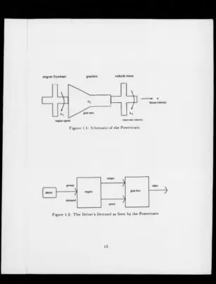
1.1 Schematic of the Powertrain... 13
1.2 The Driver’s Demand as Seen by the Powertrain... 13
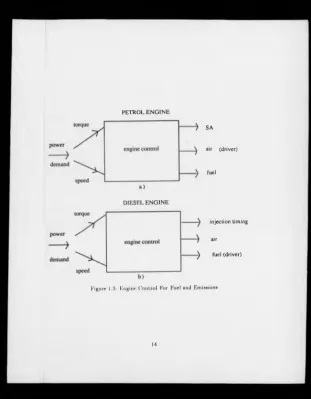
1.3 Engine Control For Fuel and Emissions... 14
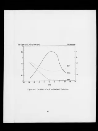
1.4 The Effect of A/F on Fuel and Emissions... 15
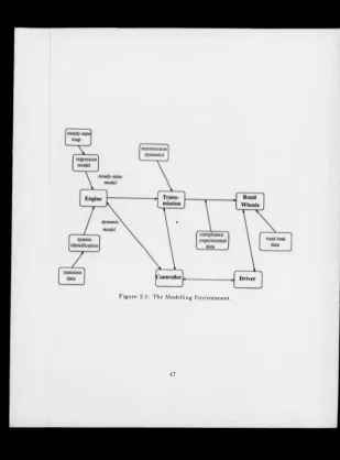
2.1 The Modelling Environment...47
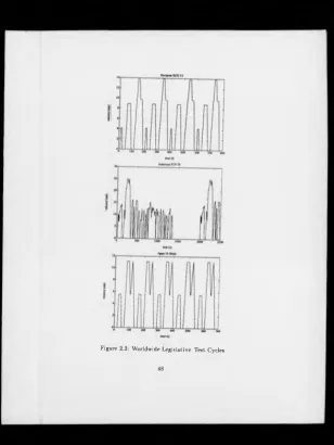
2.2 Worldwide Legislative Test Cycles...48
2.3 Tractive Effort Characteristics of Traditional Gearbox and CVT . . . 49
2.4 Regression of Engine Characteristics ...50
2.5 Fuel Contour Map ...50
2.6 Particulate Contour M ap... 51
2.7 NOx Contour M a p ...51
2.8 H.C Contour m ap...52
2.9 Smoke Contour M a p ...52
2.10 Rolling Resistence of Vehicle...53
2.11 Engine Characteristics... 53
2.12 Schematic of Powertrain Model ...54
2.13 Schematic of Compliant Powertrain M odel...54
2.14 A More Representative Model For Compliant Powertrain...54
2.15 Vehicle Speed Response ...55 2.16 Engine Speed Response . . . .
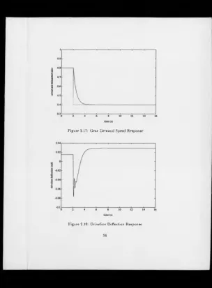
2.17 Gear Demand Speed Response 2.18 Driveline Deflection Response 2.19 Driveline Torque Response . . 3.1 Nonlinear Servomechanism 3.2 Jump Resonance...
3.3 A Classification of Nonlinearities ...91 s
s
ss
g
a
z
t
z
z
z
z
z
z
z
3.4 Separable and Nonseparable Nonlinearities...92
3.5 Schematic of a Piecewise Linear Phase Plane...93
3.6 Single Objective Optimisation...94
3.7 Steepest Descent Optimisation...95
3.8 Nonlinear Function Showing Non-Convexity...95
The Role of the Scheduler...130
The Interaction of the Scheduler and Controller...130
The Scheduling Process...131
The European ECE-15 Test Cycle...132
The Inverse Model Approach...132
Schematic of Economy Line Formulation of Minimum S F C ...133
Fuel Contour Map ...133
Particulate Contour M ap... 134
NOx Contour M a p ...134
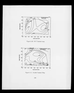
4.10 H.C Contour m ap...135
4.11 Smoke Contour M a p ...135
4.12 A Representation of Fuel Flow Optimisation In 2 -D ...136
4.13 A Representation of the Optimisation Constraint Surface In 3-D . . . 136
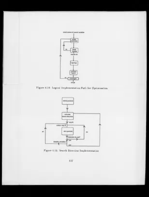
4.14 Logical Implementation Path for Optimisation...137
4.15 Search Direction Implementation...137
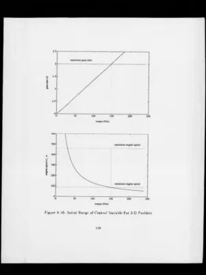
4.16 Initial Range of Control Variable For 2-D Problem...138
4.17 Single-Objective Solution Points for Fuel Minimisation...139
4.18 Fuel Optimal Schedules... 139
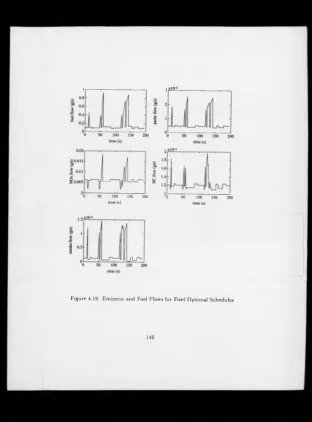
4.19 Emission and Fuel Flows for Fuel Optimal Schedules ...140
4.20 Shallowness in the Optimisation Contours ...141
4.21 Single-Objective Solution Points for Particulate Minimisation...142
4.22 Particulate Optimal Schedules...142
4.23 Emission and Fuel Flows for Particulate Optimal Schedules...143
4.24 Single-Objective Solution Points for NOz Minimisation...144
4.25 NOx Optimal Schedules...144
4.26 Emission and Fuel Flows for NOx Optimal Schedules...145
4.27 Single-Objective Solution Points for HC Minimisation...146
4.28 HC Optimal Schedules...146
4.29 Emission and Fuel Flows for HC Optimal Schedules...147
4.31 Smoke Optimal Schedules...148
4.32 Emission and Fuel Flows for Smoke Optimal Schedules...149
4.33 Possible Sources of Error in the Formulation...150
5.1 A Graphical Interpretation of Multi-Objective Optim isation...179
5.2 The Set of Noninferior Solution P o in ts...180
5.3 A Graphical Interpretation of the Weighted Sum M ethod...181
5.4 Non-Convexity of the Trade-Off Space ...181
5.5 Solution Points for Weighted Sum (Equally Weighted)... 182
5.6 Solution Points for Weighted Sum (HC Emphasised) ... 182
5.7 A Graphical Interpretation of the e-Constraint M ethod...183
5.8 The Feasible Region Imposed By Emission Constraints (. . Exterior of Boundary) ... 183
5.9 A Graphical Representation of the Goal Attainment M ethod...184
5.10 e-Constraint Solution for Loose Limits (. . Exterior of Boundary) . . 185
5.11 Schedules For Goal Attainment : Equal Weights, Mean Goals . . . . 185
5.12 Fuel and Emissions For Goal Attainment : Equal Weights, Mean Goals (- optimal flow g/s, - - mean limit level g /s )...186
5.13 Schedules For Goal Attainment : NOx Weighted, Mean Goals . . . .187
5.14 Fuel and Emissions For Goal Attainment : NOx Weighted, Mean Goals (- optimal flow g/s, - - mean limit level g /s )...188
5.15 Schedules For Goal Attainment : Partic. Weighted, Mean Goals . . . 189
5.16 Fuel and Emissions For Goal Attainment : Partic. Weighted, Mean Goals, (- optimal flow g/s, - - mean limit level g/s) ... 190
5.17 A Comparison of Particulate and NOx Solutions For Mean Goals . .191 5.18 Schedules For Goal Attainment : Equal Weights, SO G oals...192
5.19 Fuel and Emissions For Goal Attainment: Equal Weights, SO Goals, (- optimal flow g/s, - - mean limit level g / s ) ...193
5.20 Schedules For Goal Attainment Method : NOx Weighted, SO Goals . 194 5.21 Fuel and Emissions For Goal Attainment: NOx Weighted, SO Goals, (- optimal flow g/s, - - mean limit level g / s ) ...195
5.22 Schedules For Goal Attainment : Partic. Weighted, SO Goals . . . . 196
5.23 Fuel and Emissions For Goal Attainment : Partic. Weighted, SO Goals, (- optimal flow g/s, - - mean limit level g/s) ...197
5.24 A Comparison of Particulate and NOx Solutions For SO Goals . . . . 198
a s
6.2 Flow Functions for Control Law Design, (- optimal flow g/s, - - mean
limit level g/s) ...230
6.3 Engine Map for Control Law Design Showing Particulate Contours . 231 6.4 Regression Points From Optimal Schedule...232
6.5 Torque and Ratio Control Laws For ECE-15 Cycle...233
6.6 Brake Control Law For ECE-15 Cycle... 234
6.7 Comparison of Optimal and Controlled Torques...235
6.8 Comparison of Optimal and Controlled Ratios...236
6.9 Comparison of Optimal and Controlled Brake Forces...237
6.10 Gear Ratio and Demand For T = 0 .1 .238 6.11 Gear Ratio and Demand For T = 0 .5 .238 6.12 Gear Ratio and Demand For T = 1 ..238
6.13 Road Load Under Dynamic Model ... 239
6.14 Dynamic Simulation of Control Laws For T=0.5 : Demand...240
6.15 Dynamic Simulation of Control Laws For T=0.5 : S ta te s...240
6.16 Dynamic Simulation of Control Laws For T=0.5 : Tracking...241
6.17 Comparison of Steady State and Dynamic Engine Speeds ...242
6.18 Powertrain Torque Balance...243
6.19 Imbalance Between Static and Dynamic Models...244
6.20 Govenor Control Scheme...245
6.21 Friction Adjusted Engine T orque... 246
6.22 Govenor Adjusted Engine Torque... 246
6.23 Control Input Demands ...247
6.24 State Variables Under Dynamic Simulation... 247
6.25 Tracking of Test C ycle...248
6.26 Function Output Under Control Laws, (- optimal flow g/s, - - mean limit level g/s) ...249
6.27 Engine Map For Control Law Simulation...250
6.28 Velocity and Acceleration Profiles For FTP-75 C y cle ...251
Modified Control Law For EPA Cycle... 252
Modified Brake Control Law For EPA Cycle... 253
6.31 Friction Adsjusted Torque Demand Over EPA Cycle ...254
6.32 Govenor Adjusted Torque Demand Over EPA Cycle...254
6.33 Dynamic Simulation of Control Law Inputs Over EPA C ycle...255
6.34 Dynamic Simulation of State Variables Over EPA Cycle...255
A cknow ledgem ent
There are many people to whom grateful thanks are due. Firstly, I am indebted to my supervisor, Dr. Peter Jones, for his continual en couragement and advice throughout this project, and for his guidance in writing this thesis.
I would like also to thank SERC and Lucas Automotive for the fund ing of this CASE project. In particular, I would like to thank Dr. P. Extance, for his encouragement, and Dr. P. Scotson and Mr. P. Ma son for their technical support and advice, and for provision of essential engine data.
Grateful thanks are due to Prof. P. Flemming, and Dr. A. Grace, previously of the University College of North Wales, for the provision of the MATLAB Optimisation Toolbox, and to Mr. T. Crummey, of University College of North Wales, for his backup help. I hope that my return comments have been useful.
C hapter 1
In trod u ction
The established methods of control theory have had a pervasive impact on modern technology, (1). The application of these well-established methods has expanded hand in hand with the growth in computer technology, together with increasing scope for the use of modern control concepts. Motivated by the need for control where the limitations of classical control theory are now recognised, especially within nonlinear dynamic systems, new approaches are being sought within the industry as a whole .
wit-ness a widespread introduction of control microprocessors, into both passenger and commercial vehicles, the resulting features of which are likely to be : integrated en gine and transmission control to improve fuel economy and driveability; automatic suspension control to improve both ride and handling; traction control combining powertrain control and anti-slip braking; and variable assist steering systems, giving firm or lose steering dependent on the need of the driver, [3], [4].
The introduction of electronics has also facilitated the growing trend towards the total vehicle control concept - a network of control systems throughout the vehicle, communicating via a Control Area Network (CAN), and possibly under the super visory control of a central microprocessor, (4). This progress towards integration of automotive vehicle subsystem controls requires that the interaction between the various subsystems be taken into account at the design stage. To achieve this a systematic approach to vehicle control is needed in order to cope with the wealth of complex interactions between the various subsystems, [2].
management in their own rights. Instead, powertrain control here is concerned with nonlinear driveline torque management across the three subsystems.
Under the conflicting constraints of user and legislative requirements, the inher ent powertrain control system needs first to determine the control inputs required in order to achieve the desired goals. This is the concept of control scheduling, and reflects the need of the control engineer to spend a considerable amount of time in the analysis as opposed to the control design stage. It is the aim of this thesis to investigate the optimum control scheduling rules for a nonlinear powertrain given the conflicting goals of the system.
1.1 Powertrain Control
The function of the powertrain is to provide the necessary forces for locomotion. Produced by the energy released through the combustion of liquid fuels such as petrol and diesel, the resulting mechanical power is translated from a speed of rotation and torque level, output at the engine flywheel, to a tractive effort at the road wheels via the transmission and driveshaft. The transmission usually consists of a clutch, fluid coupling or torque converter to provide a means of decoupling the engine from the drive wheels during a gear change, or when the vehicle is at rest, together with a gearbox.
second type offers a continuous variation in gear ratio within the upper and lower bounds of the system and are automatically controlled. The inherent fuel econ omy improvements which in principle result from the use of continuously variable transmissions, (C.V.T.), make it increasingly attractive, [18].
Based on a perceived vehicle speed and road conditions, the driver will make a demand, which is transferred to the engine as a power demand. Figure 1.2. The outputs from the engine subsystem, as seen in the Figure, are engine speed and torque at the flywheel. These are then modulated so that the demanded power requirements are achieved, as well as other system objectives. These include good driveability - the response and ease of handling of the vehicle, fuel economy and low exhaust emissions. On passing through the transmission and road wheels the selected torque must also produce the desired vehicle speed.
The parameters of the modulation process are thus dictated by the user’s require ments and increasingly by worldwide legislation. Drivers have always demanded good fuel economy and performance, but wider political issues, such as the oil crisis of the 1970’s and erratic prices changes of the 1990’s, renew the interest in produc ing fuel efficient vehicles. Increasingly important however, has become the need to reduce vehicle emissions. Environmental concern, and increasing consciousness of their damaging effect to health, has meant that emission reduction is at the forefront of design issues.
de-sign has gone some way towards improving emissions, (7], as have the developments of lean burn engines, catalytic converters and exhaust gas recirculation, (E.G.R.). Reductions due primarily to engine design can be seen for a diesel engine in Table 1.1. The figures compare two standard commercial vehicle engines, and the values given are the simulated minimum possible emissive output for each function over a prescribed driving cycle, for equivalent vehicle model parameters. The newer data represents a more modern engine incorporating a turbo-charger and E.G.R. . Also shown are the equivalent legislative limits for the respective test. It is still not pos sible to meet the stringent limits for nitrous oxides on the newer engine even with improved engine design and exhaust gas recirculation.
Any control applied to the problem is very much dependent on the type of fuel used and the subsequent engine’s design. Control of petrol fueled or spark ignition, (S.I.), engines is dependent on the driver varied throttle angle, which determines the air intake, the metering of fuel and the adjustment of the spark timing, Figure 1.3a. The total quantity of air and fuel supplied affects the level of torque produced and the ratio of air to fuel (A/F) influences the smooth running, the fuel economy and the exhaust pollutant formation. Figure 1.4 provides a quantitative description of the effect of A/F on fuel economy and exhaust emission levels in a typical S.I. engine, [8]. The trade-offs between the objectives can quite clearly be seen and precise control of A/F ratio is necessary for optimum performance of the engine. For a S.I. engine this can be achieved by running the engine lean or through exhaust gas after-treatment devices, or a combination of both, [9j.
to avoid soot and hydrocarbon production, and the engine condition range in which it must run for good efficiency is far narrower, [8], engine control is more restricted. The previous methods of lean burn and exhaust gas after-treatment, which operate around stoichiometry, are not appropriate and control is forced away from the engine to the more general control of the powertrain.
The legislation which restricts the emissive output of the vehicle is based on standard driving cycles. Three general configurations exist, the European E.C.E., American F.T.P. and the Japanese cycle. Each attempts to reflect the habitual driving styles of the respective continents. The tests generally cover the whole operating range of the vehicle which is important since some operating conditions are more onerous than others. For instance, for a diesel engine, a greater part of the nitrous oxides are formed in the high load/high speed area, whereas the high speed/light load operations are deemed to enhance emissions of hydrocarbons and lube oil particulates, [6, 7]. Acceleration phases normally cause increased emission of black smoke, whilst motoring phases are thought to be an emissive source of unburnt lubricant, [6]. The minimisation of particulate output is especially challenging for the automotive industry which faces reductions of around 60% of current American levels by 1994 legislation, [6].
manipulations have been numerous in recent years. These are summarised fully in Tennant and Blumberg, [11, 12], with modelling approaches summarised in Powell, [14], and discussed more fully in Chapter 2. The treatments involve a mix of on-line and modelling techniques together with the application of control. Traditionally adjusted by mechanical carburettors or distributors which change only in response to engine conditions, digital electronic controllers now allow the optimisation of the running state to be adjusted so that any particular speed and torque output can select any spark advance or air-fuel ratio.
Optimal transmission scheduling, the second approach is available to both S.I. and diesel-engined vehicles, and involves the modulation of torque across the power- train in order to meet the demands of low fuel, low emissions and good driveability. This has traditionally involved treating the drive cycle as a number of steady state operating points, [13] and using inverse kinematic models to drive the vehicle up the ‘economy line’ - the locus of optimal steady state speed-load points. Analyses have been undertaken in both the discrete gearbox domain, [13, 16, 17] and for that of the continuously variable transmission, C.V.T., [18, 19, 21], although many of the principles are interchangeable. Discrete transmission control can further be classified according to whether gear scheduling and or gear execution is controlled,
P ) .
time-dependent process rather than approximated to a discrete number of either ve hicle speed/acceleration or engine speed/load demand points. The omission of such transient effects has consequences on the accuracy and applicability of the results but the role of finite-dimensional studies in the control process is such that it lays the foundation and input to more complex dynamical control.
Both approaches to the emission control problem have covered the two central themes of control. The first is concerned with closed loop control and feedback principles. For engine control this includes the feedback control of idle speed, after exhaust emissions and spark advance, and includes intelligent control methods such as adaptive and predictive control, [15]. The second approach is open loop control formulated by optimal control principles and generally makes use of search methods and Lagrange Multiplier theory.
The overall goal of either control approach is to provide the best fuel economy and emissions output together with acceptable driveability. It is the optimal control approach however, that is pertinent to powertrain control scheduling, and is the approach taken here. That is, to transfer the demand of the driver into a computed gear ratio and engine torque which when achieved by the actuator, will result in the desired vehicle speed. This modulation of the power demand, termed powertrain scheduling, is, as stated, an approach applicable to both S.I. and diesel-engined vehicles.
Previous attempts at applying optimal scheduling to powertrain control have al most exclusively consisted of finite-dimensional approximations at discrete speed/load points. The finite-dimensional formulation presented here, will be seen to produce not only acceptable vehicle control but also provide the fundamental building block to more dynamic optimisation studies. Use of this finite-dimensional information allows a more formal approach to the dynamic problem, [22, 23].
The most important flaw of previous work however, is the treatment of the con trol objectives, specifically that of the fuel and emissions. All previous work has applied the minimisation process to one of the objective functions only, writing the remaining objectives as constraints on the optimisation. As discussed, a trade-off is unavoidable between the full set of objectives, and this cannot be fully exploited by previous formulations. As such, analysis of the trade-offs has to be done manually for the full extent of the compromise space to become apparent. The true optimisa tion environment is one of minimising many contending objectives simultaneously. This can be done by making use of well established multiple-objective optimisation procedures, [24], which are used extensively in manufacturing and socio-economic spheres. Application to control has until now been limited to compensator design, [82]; applied to the fuel and emission minimisation process of optimal scheduling, these methods can be encompassed into an interactive computer tool capable of producing trade-off solutions, the exact nature of which are dependent on the spec ifications of the engineer and legislative restrictions.
produce the best fuel and emission production given the demands of the driver. If implemented in a finite-dimensional regime, the results not only stand up for themselves in terms of implementable gear schedules, but also lead into infinite dimensional formulations which include time continuous transient effects, especially important for C.V.T. vehicles. Most importantly however, the inherent objectives of fuel and emission minimisation, given that the driver demand must be satisfied, can be formulated as a multiple-objective optimisation problem, the result of which is a trade-off solution to gear scheduling without time consuming manual analysis.
1.2 Aim s and Scope
The general aim of this study is to apply nonlinear techniques to automotive con trol problems, specifically the problem of fuel and emission minimisation. This is undertaken through powertrain scheduling and control, using nonlinear optimisa tion techniques and the novel application of multi-objective optimisation methods. Steady state optimisation of the powertrain and dynamic simulation of such will allow rule-based control laws to be formulated.
The study here is specifically applied to a diesel-engined vehicle containing a C.V.T. . The powertrain scheduling approach applied to diesel engines is itself novel, but is not restricted to this alone, and as will be discussed can be used for other engine and transmission types.
The powertrain is inherently nonlinear and unsuitable to linear analysis. Chapter 3 therefore discusses the possible elements of a nonlinear system, classifies them, and introduces some of the techniques available for their analysis. Particular emphasis is given to optimisation methods, the basic techniques of which are discussed in some detail. The discussion is restricted to finite-dimensional optimisation.
Chapter 4 develops the optimisation formulation for the scheduling problem, using methods discussed in Chapter 3. The environment is single-objective opti misation, each fuel or emission function minimised separately. This, together with the use of constraints on the other functions, is the classical approach to powertrain scheduling. Here, it will be used as a first pass solution to gain knowledge of the underlying complex interactions of the system and to give motivation to the use of multi-objective optimisation methods.
The application of multi-objective methods to the scheduling problem is dis cussed in Chapter 5. The three basic techniques : Weighted Sum, s-Constraint, and Goal Attainment, are used for the fuel and emission minimisation problem, and the applicability of each discussed. Particular emphasis is given to the Goal Attainment method, which is used in Chapter 6 to develop the scheduling problem and to for mulate a control scheme which is able to both dynamically track the test cycle and reproduce the optimality of the resultant schedules. Dynamic simulation is used to measure how far these have been achieved. Finally, the driveability of the control scheme is discussed together with simulation studies to test its sensitivity to varying test cycles.
(9)
Old Data New data Limit
fuel 112.16
109.22
-part 0.20
0.26
0.338
NOx 2.70
1.5
1.28
HC 0.65
0.27
1.0
engine flywheel gearbox vehicle mass
* 3
[image:27.335.17.324.12.416.2]rotational velocity
Figure 1.1: Schematic of the Powertrain
PETROL ENGINE
DIESEL ENGINE
SA
air (driver)
fuel
injection timing air
[image:28.335.12.323.19.418.2]fuel (driver)
C hapter 2
M od ellin g and C ontrol o f
A u to m o tiv e P ow ertrains
2.1 Introduction
There are many incentives for the use of modelling and simulation in engineering development work; not least of which is the reduction in time and cost of such work and the assessment and attainment of more optimal design configurations, [13].
The choice of mathematical model for a given system is crucial to the resultant control analysis and design. It should reflect the important characteristics of the system while neglecting those over-complications which will only hinder the control analysis and design process. Most successful applications of control theory are based on simple mathematical models, and the models presented here will only reflect the relevant components of the powertrain and their interactions, not their utmost detail.
Previous modelling approaches can be classified into engine modelling; transmission modelling, often as a part of complete powertrain models; and modelling of other subsystem units, such as decoupling devices. Approaches to spark ignition, (S.I.), and diesel-engined vehicles will be discussed, together with the two facets of control : optimal scheduling and feedback.
The primary aim of the models presented here, is to formulate the powertrain control problem of transferring the demand of a test cycle, in the form of velocity and acceleration trajectories, into an engine torque, gear ratio profile. The logical flow of the model must thus be to take a velocity and acceleration input at the tyre/road interface, to transfer this back through the gearbox, and then to establish the engine power demand. The formulation here thus closely follows the inverse modelling approach taken by Blumberg, [13], although the exact powertain configurations differ.
degree of nonlinearity inherent in the driveline will be shown through simulation, by observing the response of the vehicle to a step input in gear ratio.
All of the models presented are for a diesel-engined vehicle incorporating a C.V.T., with model and constraint data obtained from engine test bed regression analyses. Some vehicle data was unobtainable for the particular test vehicle and estimates based on previous studies have been used. Although the type of engine- vehicle configuration will have implications on the resultant control solutions, this does not restrict subsequent analyses. The models are equally applicable to other engine and transmission types, given the relevant data. The consequence of in cluding a diesel engine or continuously variable transmission are expanded upon in Section 2.3.1, where the aim and scope of the models is also discussed.
Each model is constrained by physically based bounds on the state and control variables, which in turn act as constraints on the optimisation of the control objec tives. That is, each vehicle model has an associated engine map which defines the fuel and emission flow over the full operating range. These fuel and emission flow maps are nonlinear polynomials in engine torque and speed, having been regressed from engine test bed data. They define the cost function which the model equations act to constrain in an optimisation environment. The extent of their nonlinearity, and the consequences for optimisation, is discussed separately in Section 2.3.2, since the objective function formulation is unrelated to the level of complexity of the powertrain model.
both objective and constraint equations has profound consequences on the optimi sation formulation, as does the recognition that there is more than one optimisation objective.
2.2 Approaches to Powertrain M odelling
Automotive powertrains can be conveniently considered to consist of several inter acting subsystems, i.e. engine, transmission, road wheels, vehicle, control system and driver, the interaction of the models of which can be seen in Figure 2.1. The approach is based upon the interaction of discrete subsystem models, derived from regression data or physical laws, linked to a controller which interacts with driver and vehicle. In general the individual subsytems are complex and result in a system which is inherently nonlinear. The analytical treatments of each have been covered to a greater and lesser extent in the literature under the different guises of perfor mance, economy and safety. Many powertrain simulations exist which are chiefly geared to the improvement of fuel economy and emission output, either by engine management or powertrain control. Specific vehicle configurations, and general pur pose models, have been developed in both the finite and infinite-dimensional regimes, although the latter are far rarer. Other classifications, [25], distinguish between the causal and non-causal (inverse model) type simulations.
vehicle speed, acceleration demand and gear shift points at discrete time intervals, nominally one second, with the dynamic nature of the test varying between cycles. The ECE-15 cycle shown, used within most European countries, and used in this work, consists of clear stages of idle, acceleration, deceleration, and cruise.
Previous modelling efforts, have attacked all areas of the powertrain but mod elling of the engine has perhaps had the most frequent appearance in the literature. Control was applied first to this area in the early 1970’s, [26] and it was not until the mid 1980’s that control of other parts of the powertrain started to catch up. The following discussion of powertrain modelling reflects this, and the fact that although every effort has been made to include the most important contributions, the inclusion and discussion of all papers is impossible. Only those pertinent to the optimisation and control of fuel and emissions are discussed in detail, and the reader is referred to such review papers as Powell, [14], and Costa, [2] for detail of other criteria.
2.2.1 Engine M odelling and Control
decade, [14]. Some authors prefer not to use models at all and work exclusively with a mixture of engine and computer hardware, in an effort to capture fully the transient nature, [39]. However, the flexibility, repeatability, and availability of engine models means that they will always be a strong feature of engine control design.
recently, Tennant et al. (1983), [12], used a test bed derived steady state engine model together with Lagrange multiplier theory to optimise fuel economy subject to driveability and emission constraints.
Feedback and modern control concepts have also been applied to engine control in recent years. Blumberg (1981), [11], used feedback of E.G.R. to reduce the emissions of nitrous oxides on a vehicle having a three way catalytic converter. Adaptive open and closed-loop control schemes have been developed by Kiencke (1988), [15], for A/F and knock control and has combined partially dynamic models with static control maps.
2.2.2 T ransm ission M odelling and Control
Powertrain control, involving shift execution and the scheduling of gears, has been much less widely tackled in the literature. Gear train scheduling, as with the former approach, is most often posed as either a fuel and emissions problem or under performance criteria. Shift execution control is usually undertaken as a means to improve driveability and performance.
For fuel and emission reduction through gear scheduling, treatments have again concentrated on the use of steady state models. For discrete ratios Thring (1981), [16], looked at the effect on fuel economy of changing the number of gears, while Wong (1979), [17], looked at shift scheduling for maximising fuel usage by optimum power matching. Both used analysis rather than optimisation techniques.
lengthy process of dynamic programming by eliminating non-optimal shift patterns. However, the method is still computationally burdensome and the nature of the search is such that only discrete points on the objective function space are tested. Although, it did incorporate dynamic effects such as shift frequency and driveability, the analysis still did not exploit the trade-offs between fuel and emissions.
Another important aspect is that neither Radtke or Kuzak explicitly considered the manipulation of engine torque and speed in their studies. Neither formulation allowed the engine torque to act as an optimised variable. Whilst Radtke’s formula tion did calculate the optimal fuel economy, it indicates the optimal ratio selection only as a function of driveshaft speed and load and only at a limited number of points. Kuzak developed vehicle implementable shift strategies based on piecewise linear approximations as a function of driveshaft speed and throttle angle, making the ratio selection a complex function of two variables.
Full dynamic optimisation of fuel economy has been undertaken by Jones (1991), (22), using the Maximum Principle, for a vehicle incorporating a C.V.T., using a two state, two control variable model. Infinite-dimensional optimisation was used to minimise fuel economy over the whole driving cycle in one pass of the optimisation, whilst also tracking the test cycle. Improvements to this initial formulation were made by Garbett et al., [23], using steady state time history solutions as suboptimal approximations to the dynamic problem.
of constraining the analysis to the positive region of the speed-torque map. Diesel-engined vehicle transmission control to reduce fuel and emission output, has until now escaped any major treatment in the literature. This may be because the diesel engine is, by nature, intrinsically cleaner than the petrol engine. However, with legislation tightening on the commercial market at as quick a pace as for the passenger car market, and with current methods unable to fully solve the particulate emission problem, [6], powertrain scheduling approaches are more valuable now than ever before.
2.2.3 O ther Vehicle M odelling and C ontrol Issues
The design and development of interactive models of vehicle subsystems also re quires the inclusion of torque converter or clutch models. The driveability problems associated with unwelcome interactions between subsystems are concealed to a great extent by the torque converter in an automatic vehicle and controlled by the clutch in a manually shifted vehicle.
2.3 The Powertrain M odel
2.3.1 Aim and Scope
The models presented in the following sections are used in subsequent chapters to simulate and optimise the vehicle fuel and emissions output over a specified driving cycle. As such, they need to translate the cycle demanded vehicle speed and acceleration into an engine torque, speed and gear ratio profile. They thus follow the inverse model methodology of Blumberg, [13]. The first is a finite-dimensional formulation using a discrete approximation to the test cycle at one second intervals, the inputs of which are therefore scalar. The second model is a more complicated infinite-dimensional formulation where the variables are now continuous vectors over time. Finally, a compliant version of the same model is presented.
The models have been kept simple for implementational purposes but are flexible enough for other dynamic considerations to be added if necessary. Engine block dynamics which have a frequency of approximately 7Hz are not included, since this is less important in a continuously variable transmission where shift changes are smoother. Dynamic engine effects associated with the combustion process and the intake of air and fuel, together with the cyclic production of torque are ignored in this model since these too are outside the frequency range of interest, and are more applicable to engine than transmission control. Also, the engine torque is assumed to be directly available as a control variable, together with vehicle braking force and C.V.T. ratio demand.
vehi-The Diesel Engine
Diesel engines due to their increased efficiency but increased noise and weight prob lems have traditionally been exploited in the light to heavy commercial vehicle market. Unlike petrol engines, which are most efficiently run at stoichiometry or lean of it, diesel engines must be run with an excess of air and at higher temper atures. Failure to do so not only causes inefficient running of the engine but also causes increased output of soot and hydrocarbons (H.C.), [8]. For a properly con trolled engine, carbon monoxide, and gaseous hydrocarbon output is relatively low. However, one of the major disadvantages is the relatively high level of particulate emission, not only responsible for the blackening of buildings, but also found to contain carcinogenic agents, [48].
The monopoly of the S.I. engine in the overall market has meant that a plethora of techniques have been developed to reduce emission output without a reduction in fuel economy. Since most of these techniques are based on the two basic variables of air supply and temperature they do not easily transfer across to diesel engines. As such, the commercial vehicle market is in a quandary as to how to achieve the ever increasing emissions legislation, and especially the stringent particulate measures due to be introduced by American legislation in 1994, [6].
The industrial nature of this project has influenced the type of data available and as such diesel engine data has been used throughout. This makes little difference to the techniques used, which are applicable to any engine design which can be characterised as engine speed and torque pairs. However, any resultant control
The Diesel Engine
Diesel engines due to their increased efficiency but increased noise and weight prob lems have traditionally been exploited in the light to heavy commercial vehicle market. Unlike petrol engines, which are most efficiently run at stoichiometry or lean of it, diesel engines must be run with an excess of air and at higher temper atures. Failure to do so not only causes inefficient running of the engine but also causes increased output of soot and hydrocarbons (H.C.), [8]. For a properly con trolled engine, carbon monoxide, and gaseous hydrocarbon output is relatively low. However, one of the major disadvantages is the relatively high level of particulate emission, not only responsible for the blackening of buildings, but also found to contain carcinogenic agents, [48].
The monopoly of the S.I. engine in the overall market has meant that a plethora of techniques have been developed to reduce emission output without a reduction in fuel economy. Since most of these techniques are based on the two basic variables of air supply and temperature they do not easily transfer across to diesel engines. As such, the commercial vehicle market is in a quandary as to how to achieve the ever increasing emissions legislation, and especially the stringent particulate measures due to be introduced by American legislation in 1994, [6].
The industrial nature of this project has influenced the type of data available and as such diesel engine data has been used throughout. This makes little difference to the techniques used, which are applicable to any engine design which can be characterised as engine speed and torque pairs. However, any resultant control
strategies will differ to some extent.
The C.V.T.
Continuously variable transmissions were used for many years in the machine tool industry and as variable speed transmissions in many small vehicles such as tractors. The automobile industry’s interest in them started in the 1960’s with periodically renewed interest since then. Most recently two major car manufacturers, Ford and Fiat, have introduced C.V.T.’s into their smaller saloon cars, with other manufac turers expected to follow.
The C.V.T. has been used in the models here not only because it is interesting in its own right but, because of its very nature, the differential equations which describe it are continuous. This makes both the optimisation formulation and control analysis easier mathematically, and in essence will give the ‘optimal’ gear scheduling solution to which manual gearboxes can only approximate. If a manual gearbox solution is required this approximation theory would have to be carried out.
variation can be defined mathematically as,
r G [ri»r3i...r„], n = l,..5,.. (2.1)
and
(2.2)
for discrete and continuous gearboxes respectively. The minimum ratio achievable is dependent on the C.V.T. used. Many incorporate torque converters or clutches which decouple the engine from the vehicle. The Perbury transmission however, can accommodate a zero minimum gear ratio, or ‘geared neutral’.
The result of such a wide range of ratios is that the vehicle is able to hug the maximum power curve at all times. With a discrete ratio gearbox the vehicle falls away from the maximum power curve at the top end of each gear ratio selection, Figure 2.3. This means that for a C.V.T. vehicle a constant engine speed can be maintained under acceleration, and can be chosen such that fuel economy or emission output is much lower.
The benefits credited to the C.V.T. thus include improved fuel economy and acceleration performance, more flexible engine and vehicle control strategies and weight-size reductions to the vehicle, [50]. Under optimisation, they produce truly ‘optimal’ control strategies compared with discrete gear sets which can only give approximate or ‘suboptimal’ solutions to the continuous trajectories.
2.3.2 Regression of Engine D ata
functions are based on engine test bed data for which regression functions must be defined.
The engine data used throughout is for a 6cyl. turbo-charged diesel engine, nominally used on a light to medium commercial vehicle, with engine capacity of 2500cc. and E.G.R. . The test-bed procedure involved the steady state mapping of fuel and emission output at each engine speed/torque point at varying fuelling levels.
Engine Characteristics
test points respectively, the peak and overrun torque curves define the available engine power at any point in time.
Fuel and Emission Characteristics
Having characterised the engine's power constraints, the fuel and emission output flow maps can be characterised from the same data. This is achieved using M ATLAB facilities in the form of user-written m-files, [51]. The programs define an orthogonal polynomial fitting routine able to produce functions of the form,
/ = <*i + <*2*1 + a3ui + a4I i2 + ajUi2 + + 07X1*«! + ... + amtii" (2.3)
for engine speed Xi and engine torque uj, [77]. The degree of polynomial, n, pro duced is defined by an input variable. Statistical analysis was undertaken to deter mine the significance of increasing the order of fit, and determination of the best fit to the data. All functions were regressed to an accuracy of at least two decimal places, and the resultant flow functions are shown in Figure 2.5 ... 2.9, with the order of regression given on the plot. The regression coefficients are shown in Table
2.2
The character of the plot is very important with regards optimisation since it is the fuel and emission flow functions which define the cost function in later analyses. The degree of nonlinearity and extent to which the function is convex will determine the type of optimisation procedure used, how well it converges and whether the ultimate solution is the global minimum. It is very important therefore to have a good graphical knowledge of the objective functions being minimised.
the bounds of the engine operating range, Figure 2.5, with the global minimum being the only minimum within this range. The NOx, and H.C flow functions were also regressed to fourth order but can be seen to be far more complex, Figures 2.7, 2.8. Both are non-convex functions and have more than one minimum within the operating range. Particulate and smoke output flow have been regressed as fifth order functions, Figures 2.6, 2.9 and again are nonconvex over a wide area of the operating range.
One problem created by the nonlinear nature of some of the functions, is the accuracy of the regression in the low flow areas. For fuel and smoke functions only, in order to obtain regressions of a high enough accuracy over the major part of the operating range, negative flow areas can result. This is a modelling anomaly, and of course cannot take place in practice. However, steps can be taken, as will be discussed in Chapter 4 to overcome this for optimisation purposes.
All the figures show functions of absolute flow in g/s rather than the more tra ditional specific flow values in g/KWh. This is due to the formulation of the opti misation problem, as will be discussed in Chapter 4. It allows the functions to be defined over the whole operating range, whereas specific-flow is undefined at zero torque.
Vehicle Characteristics
2.3.3 Finite-D im ensional M odel
Engine Power and Model Constraints
The finite-dimensional model discussed here, is described as such because of its role in subsequent optimisation formulations. The model is used to determine the relationship between the instantaneous driver demand, assumed constant over a sufficiently small time interval St, nominally one second, and the power demand at the engine needed to achieve it. Thus, time is not explicitly involved in the equations.
The available power from the engine can be characterised by a peak torque and overrun curve as in Figure 2.11, and expressed mathematically as,
of this function with the rest of the vehicle model is discussed in Section 2.3.3.
where X(, and xf, are where the respective peak torque curve changes occur, and where
The available engine power is further constrained by physical bounds on the engine
Ulmin(Xl) < «1 < (2.4)
where engine torque, u1? is a function of engine speed, such that
(2.5)
speed *1,
* i mi, < X 1 < X i m„ (2.7)
Model regression parameters, as discussed in Section 2.3.2, and constraint values are shown in Table 2.1, together with gear ratio bounds as expressed by,
where the gear ratio is defined as output over input shaft speeds. The application of a braking force can be modelled by a variable U3 which is again dependent on physical limits such that,
where g., in this case is the tyre/road adhesion coefficient and A/ and g are the vehicle mass and gravitational acceleration in kg and m/s* respectively. The exact value of the maximum braking is shown in Table 2.1, for an approximate adhesion coefficient of 0.4 corresponding to a wet road. The maximum brake force limit used here is thus somewhat lower than that possible for a dry road with good tyres when
is around 0.8.
The Vehicle Model
The powertrain model can be shown schematically as in Figure 2.12, where the external forces acting on the vehicle are the reaction to the tractive force generated at the tyre/road interface and the road load and brake retarding forces. The road load term is the sum of the rolling friction and aerodynamic drag forces and is a
X
2
miD— X? —
x2
mt. ( 2 .8 )function of the vehicle speed,
Ri{v) = A + Bv + Cv3, (2.10)
where t> is the vehicle speed in m/s and A, B, and C are regression parameters as shown in Table 2.1. Gravitational effects are ignored in this model. The torque output at the gearbox, ug, is thus dependent on the road load, any braking force ap plied, and the force to accelerate the vehicle at a demanded acceleration, t>, reflected through the wheel and final drive ratio,
for brake force u3 (Newtons), and fi, a combination of wheel radius and final drive ratio, both shown separately in Table 2.1. The gearbox output torque must be balanced at the input to the gearbox by the torque at the flywheel ui (Nm), hence
where x2 is the selected gear ratio. Translating the linear motion of the vehicle into the rotational speed of the engine xt (rad/s) gives,
ug = fiRt + ftu3 + fiMv, (2.11)
u i = hx2(Mv + Ri + u3), (2.12)
V — HXiXi
, (2.13)and equation 2.12 can now be expressed as,
Since the road load, and tractive effort to produce the required acceleration are known, given an instantaneous demand in vehicle speed and acceleration, the development of the required engine power becomes a non-unique choice of engine torque and engine speed. The problem is thus one of optimisation - choosing an engine operating region and thus gear ratio which satisfy the power requirements and subsequently minimise a predefined cost function. The model is thus ideally suited to the finite-dimensional optimisation of a vehicle tracking a specific test cycle. For control purposes engine torque ui, gear ratio x2 and brake torque U3 are available to modify the power output of the engine and the resultant tractive effort at the road surface. The specific formulation of this is discussed fully in Chapter 4.
2.3.4 Infinite-D im ensional Vehicle M odel
Non-Compliant Model
The dynamic powertrain model is basically of the same nature as the steady state model just discussed, and is still modelled schematically as in Figure 2.12. The significant difference is that the models, rather than containing variables assumed constant over the interval of time 6t, now vary with time. The dynamics of the gearbox and flywheel are thus no longer negligible and are included in the model.
order lag, with unit gain, such that,
(2.15)
i.e. the difference in demanded and actual gear ratio at time t, for a time constant
of Tc. Conservation of energy across the powertrain leads to the state equation,
The engine torque is thus balanced by the road load and brake forces translated through the gearbox, and by the momentum change within the rotational elements of the C.V.T., denoted by the term,
due to the continuous ratio variation. The efficiency of the CVT is assumed to be ideal due to the lack of appropriate data.
An inverse dynamic model can also be constructed, as in the previous section, where the velocity and acceleration demand is known. The model can then act to constrain the cost function
under dynamic optimisation, where f(xi,u\) is a fuel or emission function. (/ + (fix2{t))2M)xi(t) = ui(<) - x2(t)xi(t)x2(t)Mn2
-fix3(t)(A + Bv(t) + Cv(t)2) - nx2{t)u3(t).(2A6)
x2(t)xi(t)x2(t)Mti3 , (2.17)
2.3.5 Dynam ic Com pliant M odel
If a mechanical element or structure experiences a steady deformation when acted upon by steady state forces it is said to exhibit compliance. The model here includes compliance in the driveline downstream of the gearbox. It is effectively modelled as a spring and damper system and shown schematically in Figure 2.13. In practice however, the compliance is made up of both compliance in the halfshaft, and de formation in the tyre as a function of vehicle speed. A more representative model is that shown in Figure 2.14, with the tyre characteristic incorporated as a damper at the wheel and with the deformation in the halfshafts acting as a spring down stream of the gearbox. For the purposes here however, the first representation is adequate since this study is primarily interested in transmission and not traction control. Experimentally, the formulations are very similar.
Incorporation of compliance effects requires two additional state variables to gether with the gearbox inertia. The variables x\ and xi are as before, but 13 is now the driveline output speed and x4 is the rotational deflection taking place along the driveline. The additional inertia of the gearbox is Ig, aggregated at the output shaft.
The bounds on state and control variables are as discussed in Section 2.3.4 and the C.V.T. actuation dynamics are still represented as in equation 2.15. The dy namics of the transmission can now be represented by
[/ + W O W ) = u,(i) - *
j(
i)*
1
(
i)*!(<)A> - *>(<)[**«(<) +
)*,(() -*
3
(<))l.
and downstream of the gearbox,
*«(0
= *i(0
*a(0
- *3
(0
. (2
.20
)for damping rate d and stiffness in the driveline, k. The spring and damping factors have been adjusted from previous experimental data, [49] for the specific vehicle mass. Equation 2.19 again represents the conservation of energy across the power- train and balances the engine torque against momentum changes across the gearbox represented by,
*a(t)*i(0*t(i)/„ (2.21)
and the aggregate driveline torque at the C.V.T. output shaft, represented by,
**4(t) + 4*i(t)*»(<)-*»(«)) (2.22)
The rotational motion of the vehicle driveline is represented as
c’M ii(l) = (tx,(()+<<(*i(f)*2(0-*3(l)))-/‘(/»+B»(<)+C»(<)i) - / ‘"3(0. (2.23)
for brake force U3, vehicle mass A/, and road load as before. The result is four nonlin ear coupled state equations with three control inputs and velocity now represented by,
= fix 3. (2.24)
constrain a minimisation integrai, typically
mm ji A/(x,,u,) + (1 - X)g(xi,v,x2)dt. (2.25)
The cost function consists of a weighted sum of a fuel or emission function together, in this case, with a driveability term which is a function of engine speed, vehicle speed, and gear ratio. Dynamic optimisation is not considered in this thesis. How ever, there is much scope for its application to the fuel and emission minimisation problem.
2.4 Dynam ic Simulation
Dynamic simulation allows the use of nonlinear dynamic models to predict the effect of changes in system parameters, control strategy or just to investigate transient performance. This section uses dynamic simulation to illustrate the nonlinear effects inherent in an automotive powertrain.
has to be used for computational efficiency and accuracy, [53].
The simulation experiment involves investigating the response of the C.V.T. powertrain to a step reduction in demanded gear ratio u2. The C.V.T. actuation time is around 2 seconds with the vehicle initially travelling at a steady speed of 6.16m/s, approximately 25 miles/hour, and with initial gear ratio 0.8. This approximates to a manual gear ratio of 3. At time 2 seconds a demanded drop in gear ratio is made to 0.4, around second gear. Braking force u3 is set to zero throughout.
The Figures 2.15 to 2.19 show the nonlinear response of the powertrain. Figure 2.17 displays the resulting C.V.T. ratio response which achieves its new value after 2s. The resulting response in vehicle speed is shown in Figure 2.15. The vehicle speed is seen to drop momentarily before rising slowly to a new value of 6.35m/s after 15 seconds. The engine speed, in Figure 2.'l^, shows the engine speed rising rapidly, then stabilizing to a slow climb. Figure 2.19 shows the driveline torque which oscillates before settling to its new value of 9.3Nm. The compliance has the effect of producing a deflection in the driveline which can be seen in Figure 2.18. The effect is seen to settle after 4s to a new steady state deflection value.
Given that engine torque, or equivalent throttle position, is held constant through out the simulation the rapid reduction in C.V.T. ratio after 2s decelerates the vehicle slightly at the expense of accelerating the engine flywheel. This is characteristic of a C.V.T. vehicle which is able to snatch energy from either vehicle or engine and place it somewhere else. This momentum transfer is contained within the nonlinear term
*1*2*2 Ig (2.26)
and in this case is seen to be giving energy to the flywheel. The result is that the engine, now seeing a lighter load on it due to the reduced gear ratio, and with the
torque level held constant starts to accelerate.
The decrease in gear ratio produces a rapid change in driveline deflection, which winds up in the negative direction. Nonlinear oscillations result and as the engine speed starts to rise the the driveline deflection settles to a constant positive value. The driveline torque shows a similar response.
The C.V.T. and driveline compliance thus show the nonlinear delivery of power to the road wheels and the resulting effect on vehicle longitudinal motion. As we have already seen the engine itself possesses a nonlinear torque characteristic, has a nonlinear fuel flow usage and emission output characteristics, and experiences external forces on the vehicle which are nonlinear in vehicle speed. The result is a powertrain model which is nonlinear in its basic form, its constraints and its optimisation cost functions.
2.5 Summary
A brief introduction has been given, within this chapter, to the previous research efTorts in modelling and control of automotive powertrains. Engine, transmission and decoupling devices were considered with recognition that most of the work has been done with the engine subsystem. The three main models used within this work for optimisation, simulation, and control purposes, were also introduced in detail. These included the powertrain model itself, the state and control bounds and the related fuel and emission functions. It was also shown how some of this data was obtained from regression analysis. Finally, a simulation was undertaken of the dynamic compliant model to aid understanding of its inherent nature.
The development of the finite-dimensional model equations, where only the in
stantaneous driver demand is considered, showed how a non-unique choice of engine operating region and gear ratio selection could be made. This poses an optimisa tion problem, such that the consequence of the choice can be monitored in order to minimise, for example, fuel and emissions. This is the essence of the optimisation problem considered in later chapters.
A
50
d,
5.50
B
0.34
d2 -449.15
C 0.0055
ei
-5.0
Te
0.5
C2
2316.2
I 0.159
¿1
-0.045
h
0.05
62
1.68
M 1800
X U n a ,460.77
Tw 0.28 * lmi„ 89.0
Td 0.275 *^2
max2.0
0.077
X 2 m in 0.0a x -0.0029
U 2 m a t2.0
a2 1.G13
0.0«3 -3.093 “3.„„ 6500
kc
318
- 0.0dc 4.69
Table 2.1: Model Parameter Coefficients