Approximations of a quadratic programming problem with incomplete information

WITH INCOMPLETE INFORMATION

A thesis

submitted in partial ful

of the rements for the Degree of

Doctor of Philosophy in Operations Research

in the

University of Canterbury by

John Andrew George

r:;j

<

.l

.

)

CONTEI'HS

ABSTRACT . 1

ACKNOWLEDGEHENTS . . 2

1. MOTIVATION. . 3

3 4 2 . 1.1 1.2 1.3 1.4 1.5 1.6 Introduction The Problem .

Relevant Characteristics of a Quadratic Function . . . .

Linear Approximation of a QP . . Baumol·-Bushnell Resul ts . . . Critique of Baumol-Bushnell

5 6 12 · . 16

FRANEWORK FOR THE ANALYSIS _{· 23}

2.1 2.2 2.3 2.4 2.5 2.6 2.7 2.8 2.9 2.10 2.11 2.12

Introduction . . . . · 23

Decision Rules . . . _{· 24}

Gradient Stopping Rules . . . 29 Variable Metric Decision Rule .

Controllable Aspects of the Model

· . 32 Structure . 34

The D Matrix. . . 35

The Size of the Problem . . .

Number of Observation . . . . .

Grouping Structure of Observations . . position of Unconstrained Optimum. Curvature . . . . More on the Homothetic Properties

of a Quadratic. . . . . .

· . 38 · 41

· . 42

· 44 · 47

· 51 3. THE SETUP AND RATIONALE OF THE EXPERIV£NTAL

SYSTEM . 3.1 3.2 3.3 3.4 3.5 3.6 3.7 3.8

Creating the QP . . . Solving the QP . . .

Generating the Observation Points . Seven Experiments . . . . Calculating the Decision Rules. Analysis of Observations . . . . .

Solving the Decision Rules . . . . Further Analysis of Observations and

Decision Rules . . . .

· 61 · 62 66 · . . 66 • • • 68 • • • 69 · 70 · 71

· 72 3.9

3.10 3.11

The Gradient Decision Rules . . . · 73

Card Output . . . . .

Variable Metric Decision Rule . APPENDIX 3.1

3.2 3.3

NOTATION . . . . INPUT INSTRUCTIONS OUTPUT . . . .

4. DECISION RULES, STOPPING RULES AND PROBLEM

CLASSES. . . . . . . .

4.1

4.2

4.3

4 .4

Introduction. . . . . .

Summary of Major Results . . . . General D Matrix (Type 1 Matrix)

-Decision Rules Results . . . .

General D Matrix - Problem Class Results.

· 73 74 75 · 76 · . 79

• 84 • • 84

5.

6 .

7.

All-negative Matrix Elements . . . . . 112

4.7 Results of Type 4 Matrix - Diagonal Matrix. 119 4.8 Results over Four r·1atrix Types . . . . . 123

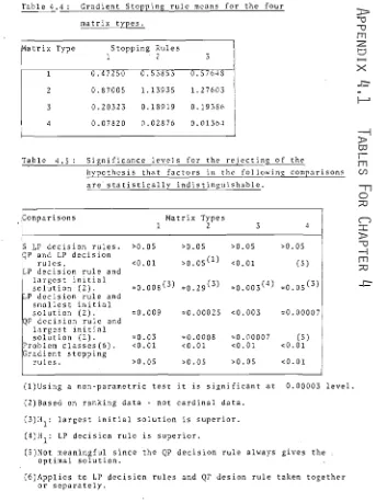
4.9 Results of Gradient Algorithm stopping Rules · 126 4.10 Results of Variable Metric Decision Rule. · 131 APPENDIX 4.1 TABLES FOR CHAPTER 4 . . · . 133

OBSERVATIONS EFFECT . . . . 5.1 Introduction . . . . 5.2 Overview of Results . . . . . 5.3 Effect of Observation Types on QP Decision Rules . . . . 5.4 Effect of Observation Types on Stopping Rules . . . . 5.5 Largest Initial Solution • . . 5.6 Number of Observations . . . . APPENDIX 5.1 TABLES FOR CHAPTER 5 CURVATURE . .

. .

,

. . . .

. . .

.

the LP and Gradient · . 162 · . 162 164 · . 166 . . . 171

. . . 172

. . . 174

· 176 · 184 6.1 Introduction. . . 184

6.2 Definition of Curvature Criteria 185 6.3 Results for the LP Decision Rule Variables. 187 6.4 Results for the QP Decision Rule . . . 189

6.5 Results of 12 Problems Studied in Depth . . . 190

APPENDIX 6.1 TABLES FOR CHAPTER 6. 198 CONCLUSION . . 202

7.1 7.2 7.3 7.4 7.5 7.6 7.7 7.8 7.9 7.10 Introduction . . . . . 202

Decision Rule Propositions. . . . . 202

Gradient Stopping Rule Propositions. . . 204

Variable Metric Proposition. . . 206

Matrix Type Proposition. . . 207

Problem Size Proposition . . . . . . . . 210

Proposition or Number of Observations . . . . 212

Observation Type Proposition . . . 213

Curvature Propositions . . . 216

Overall Conclusion . . . . . . . . . 220

ABSTRACT

This thesis deals with the effectiveness of various decision rules derived to approximate the objective

function of a quadratic programme. The assumption of the study is that the constraint set of the QP is known precisely but the objective function is known only from the data of various observations made of that function. Various

decision rules, some linear and some non-linear, are used to derive from the data objective functions to approximate the true but unknown function.

A series of problems are generated to test the

effectiveness of these decision rules. The problems are. stratified according to the nature of the true quadratic function and the size of the problem in terms of the number of constraints and variables. In addition to comparing the decision rules with each other the study also considers the effects of the type of quadratic function (matrix type), the size of the problem, the number of observations, the scatter pattern of the observations and the curvature (degree of nonlinearity) of the quadratic.

In general the decision rules do not behave well except when the curvature is very slight. In most other cases the nonlinear decision rules give much the best

results and particularly if the observations are scattered close to the true contrained optimum. The overall con-clusion is that i t 1S well worth the effort to obtain an

ACKNOWLEDGEMENTS

It is impossible to acknowledge all the people who

to the completion of a document such as

this. Some do, however, stand out.

I would I to dedicate this thesis to a quality and

a person: To perseverance - it may not be a great

of work but, after many years, i t is fini

To Roberta, my wife, who continued to I

me despite the pressure and evidence to

contrary.

My thanks go to my parents, family and colleagues

who 1 the support in different ways. arly,

Hans lenbach and Tony Rayner have supplied a great deal

of comment, help and encouragement. Also I

CHAPTER 1 MOTIVATION

1.1 Introduction

The operations research analyst, having investigated the nature of the problem on hand has next to dec on the mathematical model appropriate for solution. On many occasions the formulation is obvious, but often

i are made either for the of computa-t viability or because evidence is to support a more complex structure. This is larly true the sphere of mathematical programming where 1 programming (LP) is used as a 'good enough' appro x ion of a non-linear problem (NLP).

LP is an attractive model structure. It s ionally because the simplex algorithm is now well developed, fast and robust, and in the post analysis of LP is extens and ly s Sometimes, therefore LP is chosen as a simpli-f ion of a more complex NLP - the non-linearity, i t is , can be ignored because i t is insignificant. At other t

estimated used by de

s suspected non-linearity cannot be

se there are insufficient data, so LP is t.

This dissertation looks at the effects, within a rather 1 ted scope, of using a more simple mathematical programming structure than is really appropriate. What are the consequences of mis-specifying the model? Is a linear structure good enough when the non-linearity is

we can sa An astute

small? Are there circumstances in which y use LP when the structure is truly non-l st will spot non-linearity but what if

there are f data or knowledge of structure to identify accurately?

The by W.T. Baumol and R.C. Bushnell

produced by 1 zation in mathematical programming",

(Econometrica~ Vol. 35, No. 3-4, 1967), and Ph.D

dissertation of R.C. Bushnell, The linear assumption &n the use of the linear programming model in Economics~ form the starting point for this dissertation. The work

a quadr

some questions about the ef function, i.e., reducing a

of linearizing program (QP) to an LP. They present some surprising results.

We will their enquiry by looking at a broader class

of c functions and assume the of

they did. The second of se extensions more data

opens up mations of

possibility of simplified QP's as approxi-true QP.

1.2 The Problem

(1-1)

Let us consider the QP defined as Max z = c'x + x'Dx

s.t. Ax < b x > 0

llows:-where x, c and bare n dimensional column vectors, D is an (nxn) dimensional negative defin lC

matrix, A is an (mxn) matrix.

Let us assume a decision-maker is with a problem of the of (1-1), but is not aware its ecise

the matrix A and vector b are known exactly. What 1S not

known is the structure of the objective function. Our assumption is that knowledge of the objective function is contained in information received by observing the

function (without error).

At an observation

x

we assume that the decision-maker observes the coefficients of the tangent hyper-plane to the objective function, i.e., the vector

h

of

(1-2) c + 2Dx

=

h

How do we use the data from the observations to

create a mathematical programming problem that approximates (l-l)? How good is such an approximation? Under what

circumstances 1S the approximation good or bad?

1.3 Relevant Characteristics of a Quadratic Function Consider the quadratic f(x)

=

c'x + x'Dx. The position of the unconstrained optimum is

(1-3) x o

=

~D -1 c (where D is non-singular).

Let

A.

be the jth eigenvalue of D. Let A be the J

diagonal matrix with the

A.

's as the diagonal elements. J

The matrix of eigenvectors is the orthonormal matrix Q such that

(1-4)

Since D is negative definite, A.<O, j

=

1,2, ... ,n. J

Consider the transformation x=Qy. The quadratic form x'Dx becomes y'Q'DQ y or y'Ay from (1-4). Hadley

[11], pp.269-72, shows that this transformation is a

quadratic form remains the same apart from the rotation. The form yl~ has its principal axes parallel to the co-ordinate axes, so the matrix Q gives the position of the principal axes of D. If q. is the jth column of Q then

J

q. is the direction vector of the jth principal axis of J

D.

(1-5)

The length of the jth principal axis of x'Dx

1

ITI:T

J

1 is

(Franklin [10] , p. 96) .

If D is a diagonal matrix then D

=

A. The eigenvalues of D are the diagonal elements, and the matrix of eigen-vectors is I, i.e., ~

=

IIDI. In this case the quadratic form x'Dx has its principal axes parallel to the co-ord{nate axes.

If D is a negative matrix (i.e., all elements are

negative) then the eigenvector associated with the smallest eigenvalue (largest in absolute value) has all positive components (Franklin [10]).

A quadratic form is homothetic, i.e., the tangent hyperplanes of the points on a straight line through the unconstrained optimum all have the same slope. This can be established easily. The gradient vector of f(x) at x

1S

Now and y is

(1-6)

\j _f

₌

_{c + 2Dx}

x

let x

=

(x 0 + yd) where d is any direction vector any scalar, then

\j f

=

c' +

x

o 0

proportional to~q, and since y 1S a scalar the slope of

the tangent hyperplane is the same for all x (x +yd) . o (Of course, the coefficients will differ for different y) .

Figure 1-1: Homothetic property of quadratic function

These properties will be used as we develop and analyse our results.

1.4 Linear Approximation of a QP

One of the most significant forms of approximation of a QP - for our purposes - is an LP. Since the constraint set is known, only the objective function is approximated. We will look firstly at the different characteristics of QP and LP problems, and then at the effect of a linear approximation of the objective function.

A comparison of quadratic programming and linear programming shows a number of important differences:

[image:10.561.102.496.218.453.2]

point. A QP may have its optimal solut at any poin-t on interior or boundary of the feas e

(ii) The extreme point with the highest objective t value of a QP need not be on same of

sible region as the optimal solution. s is illustrated in Figure 1-2. In linear the

st extreme point is an optimal solution and lies on the same facet as all other optima.

1-2: Best

Best extreme point

extreme

facet of feas / /negion. that / QP optlmum

A xl

int

(iii) The simplex method always goes to an extreme nt for an LP.

A optimum of a QP is unique if the matrix D teo

(v) In general, an optimal solution to an LP is reached a fraction of the effort required to find optimum a QP

Turning to the effect of linearization, we will look at this stage at some of the more obvious results. For the problem of Figure 1-2, all of the feasible region inside the large level curve glves a better objective function value than any of the three extreme points 0, A and B. When we linearize the quadratic using for the objective function the tangent hyperplane at an observation i t is therefore likely that the LP solution will be inferior to the solution at the observation, in ter~s of the quad-ratic function. In this simple case we can tell the parts of the feasible region that will send an LP to each of the extreme points. The ray L is the set of points which have the same tangency as the constraint line. All feasible points to the left of L generate LP's (as described above) that have A as their optimum, while all points on the right of L have LP's with B as their optimum. Points on L

generate LP's that have A and B as alternative optima -but i t is not possible to choose between them or to pick the true optimal non-basic solution (which is also one of the alternative optima of the LP) . It is interesting to note that no feasible points would send an LP to 0 - the best extreme point.

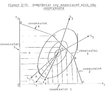
Let us illustrate this reasoning with a ~ore complex 2 dimentional problem. In Figure 1-3 we consider the rays that correspond to each of the constraint lines, i.e., L. is the ray from the unconstrained optimum, which

1

contains the points with the same slope as constraint i. There are two rays with this property - one on either side of the unconstrained optimum.

condition (1-7):

We will choose L. to satisfy

(1-7) I f x. E L., then

l l

ith constraint.

l

a x.

l

l

< 0, where a x < b.

l lS the

Condition (1-7) can be interpreted as saying that the direction of the ray L. is a feasible direction for

l

l

constraint i from the hyperplane a x

=

b ..

l

Figure 1-3: Homothetic ray associated with the constraints

constraint

5.""

-A

constraint 2

I A

~~--~--~~----~~~---~l

! .

constralnt 1

The feasible region in Figure 1-3 lS divided by the L. rays into those sections which send an LP - using the

l

tangent hyperplane at the feasible point as its objective function - to each of the extreme points. In this case there is a small region which sends an LP to the origin.

(If the unconstrained optimum is in the non-negative

[image:13.561.81.499.230.593.2]

We will return to a more detailed analysis of the homothetic nature of the QP in Section 2-12.

There is a related problem with linearization. n

2 Consider the function f(x) = L: c.X. + d. x ..

j=l J J J J c.

Its global optimum is at x 0

,

where x. = 0 J for each 2d.

J

J

(Le., when af (xo) 0) . If have observation

J _ax. = we an

J

- - 0 af

point x, with x. >x. for some j , then

ax. (x) < 0, i . e. , J J

J

the objective function coefficient for x. in the LP is J

negative for that observation. This means x. will be zero J

at the LP optimum - even though the optimal QP value for that variable is non-zero. This result is caused solely by the position of the observation point.

For the more general quadratic functions the situation is slightly more complicated. The position of the principal axes control where a point must be for one of the variables to go to zero. Figure 1-4 illustrates this. All points ln region A give xl a negative coefficient in the LP objective function, while all points in B give x

2 a

negative coefficient. We can say, however, that if X.»x. - 0 J J then very likely x.=O at the associated linear programming

J optimum.

The consequences of this conclusion are most

F

--~---~\---.----~~--- x

1

1.5 Baumol-Bushnell Results

Let us look now at Baumol-Bushnell

[1]

and

B shnell _u [2] _. Sl'nce they are cruc 1 groundwork for this dissertation we will consider them in some detail.

The framework is a quadratic function over a linear constraint set. They use the special quadratic function

(1-8 ) IT

=

n

E

j=l

2

(c.x.+d.x. ) + K J J J J

(where c

j and K are positive and dj is negative), and cast

their analysis in economic terms with the objective function being a profit function and the constraint set being

resource restrictions. They use the idea of taking a point (an observation) and estimating from the data

direct r work towards the analysis of six propositions

( 1) A 1 ar approximation to a non-linear program not necess ly yield the true maXlmum.

( 2) 1 approximation need not provide an answer

r a randomly chosen initial point.

(3) It may not even provide the best possible corner

(4) A ion in the curvature of the profit sur e s not always guarantee improvement in the accuracy of a 1 approximation.

(5) Proximity of the initial point to the maximum need not rease the accuracy of the linear approximation.

(6) Only if the objective function is monotonic throughout can we be assured that a linear approximation will yield re ts which represent an improvement over the 1

po

To test these hypothesis, over 300 quadr c

are constructed. They are grouped according to the s

of various parameters in the system, in ular the size of the elements in the constraint matrix and the pos ion of the initial point relative to the uncon optimum and constraints.

Two ways of estimating the linear are used. The st uses the tangent hyperplane at ini al point as the LP objective function. So the ve function

ients for point x :== _(x

l ,x2,···xn) are given by: (1-9) a. :== c. + 2d.x.

J J J J

(1-10) a. IT J _x. J

- 2

where IT

=

L(C.X. + d.x.) Since the objective function

j J J J J

of an LP is not a~fected by a multiplicative constant the a. coefficients can be defined as

~.

x. J J

Equation (1-9) is justified as a marginalist approach to using the data from the observation x. This approach assumes that the marginal coefficients observed at x are the coefficients of a linear function. Equation (1-10) is an averages approach which gives a unit of x. a coefficient

J

equal to the average profit. An LP using (1-10) gives a total profit of nIT at the initial point and a coefficient of the objective function of the LP inversely proportional to the relative size of x

k to the rest of xj's. The overall result of their study is:

"In general, the linear programming calculations

did not yield results very close to the true maximum nor did the approximation improve

substantially as the curvature of the objective function was reduced."

(Baumol & Bushnell [1], p.447)

On average the linear programming optimum is not only considerably inferior to the quadratic programming optimum, but yields a loss (a negative value of the true profit

function) (1-11)

The statistic used to make this comparison l S :

profit at LP optimum profit at QP optimum

The mean value of this statistic lS -9.7106 with a

In comparison to the initial point the LP optimum also fares badly. Here the statistic is:

(1-12) difference in profit between LP optimUP.1 and initial point profit at initial point

In this case the mean is -10.9720 and standard

deviation 48.6330. The theoretically best value is zero. These figures give the conclusion that, on average, the use of linear programming leads to a decrease in profit over the existing position.

A number of explanations are investigated for the overall results and differences in results for different classes of problem. The only explanatory variable of value

' t h t ' (number of non-slack variables)

1S e ra 10 _nu mb _{er 0} f _{cons ra1n s} t ' t . This gives a correlation coefficient of -0.5229 with the statistic of

(1-11) and -0.5241 with the statistic of (1-12).

Curvature is very disappointing as an explanatory variable. Neither of the two curvature measures proposed give significant results. In fact, the first measure gives a correlation coefficient of the "wrong" sign - suggesting that performance of the linear programming approximation improve slightly with increased curvature.

Analysis by Bushnell [2] subsequent to Baumol and Bushnell [1] explains the results almost entirely in terms of the position of the unconstrained optimum and the initial point. Three different procedures are used to generate

the quadratic objective functions. When these procedures are compared, the differences reduce to whether the uncon-strained optimum is outside or inside the feasible region and whether the initial point vector is less than the

is less than the unconstrained optimum which is in turn outside the feasible region the results are good

-t mos-t of -the linear programming op-tima co ded with the quadratic programming optima. An uncons ned

imum within the feasible region is the lC

programming optimum and will almost never coinc with the imum of the LP.

1.6 Cri of Baumol-Bushnell

The substantive contribution that Baumol and

have made is to establish that mild non-lineari es can, if they are ignored, cause significant dis ons

the solution of mathematical programming problems. s is in contrast with most other situations where mild

non-linearities are encountered. The reason

1 s in the special nature of the optimum

fference an LP, i.e., a basic feasible solution or an extreme point.

Two matters left unanswered by them are is s present dissertation. What bias is there in the

re s due to the rather simple quadratic function assumed Can more accurate results be obtained if more one observation is available?

11 correctly sees the position of the uncon-stra optimum as an important factor in explaining his re ts. However, i t is so good an explanation, as to r se susp ion about the validity (or scope) of the results.

ng noted that an unconstrained optimum aside the feasible region re s in a poor linear approximation, Bushnell

"Those problems did astoundingly well. The 49 cases of problems 802-851 yielded on the average 95% of their potential improvement~ Thirty-five of the 50 cases (70%) even had as their quadratic solution points the precise solution points

determined by the approximating linear program. The 48 cases of problems 852-901 yielding

improvement achieved on the average 97% of their potential improvement. 31 of the cases (62%)

had as their quadratic solution points the precise solution points determined by the approximating linear program." (Bushnell [2] p. Vl-38).

Of the other 150 problems he comments:

" ... in problems 1-50, 51-100 and 401-450 all 25 of the problems which did yield improvement hit the target perfectly ... that is to say, there 1S no

difference between the linear programming approximation and the quadratic programming solution. This apparently fantastic result occurred simply because the feasible region was

so constricted that relatively little change from the initial point could occur."

Bushnell [2] , p. Vl-40).

To Bushnell i t 1S no surprise that a non-linear problem

results of ems 802-901 in terms of the uncons ned optimum outside the feasible region and ly

few negat linear programming coefficients. This is, however, mere

well outs

saying that the unconstrained optimum is sible region - or that the level curves are "ne " by any meaningful criterion, This s Ie

would cause both a higher probability of a corner point solution, (if the quadratic programming optimum is

not a corner point) near optimal values for the corner points near the optimum of the quadratic program (see the sis of Chapter 2 of this dissertation). But is this

of the prog also

optima co Ie po

whole answer? It certainly does not answer why 150 problems (many of which had quadr

optima inside the feasible region) 25 c programrning and linear programmi iding. Bushnell's suggestion about the ion being highly constrained around the

s not tell the whole story. It would be neces ial

for the i al point not only to be near the boundary of the feas Ie set but also to be close to a corner

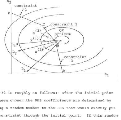
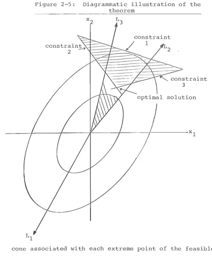
or corner points and even that is not sufficient. 1-5 illustrates this. Point x(l) in Figure 1-5 s

its LP to the optimum of the QP - but x(2) does not nor s x(3). In fact the LP from x(3) goes to corner point A a long way from the optimum of the QP. The trend

in F 1-5 is compounded considerably as the sions of increase.

The explanation probably lies elsewhere.

Figure 1-5: Initial point close to boundary

x

constraint D

2

constraint

/ 3 /

p.Vl-32 is roughly as follows:- after the initial point has been chosen the RHS coefficients are determined by adding a random number to the RHS that would exactly put the constraint through the initial point. If this random number is small, the constraints are all bunched closely around the initial point - and thus create corner points all close to that point and perhaps many redundant constraints. It is not surprising then that the optimal corner point

is close to the initial point. Also since the unconstrained optimum is also very close for these 150 problems i t is

likely that the QP optimum finds a solution at one of the corner points clustered there.

The second factor that enhances the results of 100 of these 150 problems is that the initial point is strictly

[image:22.561.109.501.124.511.2]

behaved" towards the feasible region. When this is added to the facts that the unconstrained optimum is close, and that there are corner points clustered in the area, the likelihood of a corner point solution is further enhanced.

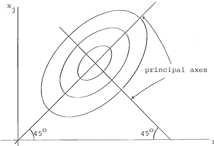
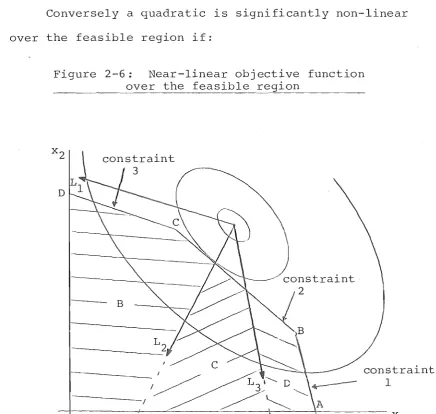
There is yet a third factor which aids good results for all the problems. The principal axes of the level curves of the quadratic functions generated do not vary greatly in length. For all 250 problems the longest

possible principal axis can be no more than 2.236 times the shortest possible. In fact they will usually be closer than this in length. The case of a very pointed level curve (as shown in Figure 1-6) is thereby excluded, yet there is the significantly "nonlinear" case (as opposed to the "near linear" case). For such a function

particularly if the principal axes are parallel to the axes -the likelihood of a corner point solution is more remote.

Figure 1-6: The pointed-level-curve case

[image:23.561.113.419.510.754.2]

It seems therefore that the results Baumol and Bushnell, though qualitatively correct and pessimistic

the value of linear programming , may not be pessimistic enough for QP's with an unconstrained

imum near, but outside of the feasib point that Bushnell says is the curious fact that the LP's he

about s are often

"

rate" (according to his terminology). He

less structural variables (non-sl abIes) non-zero value at the optimum to the LP

maximum tted by the basic theorem of programming. He c this to be "surprising". His error is s

s abIes are perfectly good variab s wi n

scope of basic theorem - and in fact neither of the examp s quoted (Baumol and Bushnell ([1], p.464) are

may, in proc

in the true sense of the term. , confirm the suspicion that his has produced many redundant constra

sobs ion

A more substantial error we have not yet ment is in their aside which seeks to find s the linear programming approximation is of

Propo 6 ( [1], p.455) conjectures that monotoni ty of

ensure

the t

1 curves over the feasible region is enough to linear program gives an improvement over solution. This proposition is then used to

provided one stays within a small area around point (thus hopefully remaining within

scope of monotonicity) the linear programming

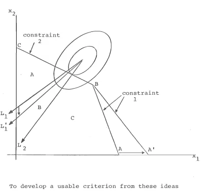
diagrammatic terms that the proposition need not be true; in i t the level curves are all monotonic yet optimum to the LP (A} is r to the initial nt x (1 ) ,

Fi Counter sition

1

In summary, Baumol and Bushnell's lem simulation procedure seems to have brought in some unnecessary bias. It seems also there has been insuf variation in curvature to meaningfully test any conjectures that compare mild nonlinearity with severe nonlineari vJhile these

CHAPTER 2

FRArllE~'JORK

FOR

HIE

ANALYSIS

2.1 Introduction

( 2-1)

fundamental problem to be analysed is: We are given the QP

Hax z

s.t.

c'x + x'Dx

Ax < b

x > 0

A and b are assumed to be known, but where the object has been observed only in the form

(2-2 ) c

+

2Dx :::: h

at a number of ,different x. How do we approximate (2 1) with a mathematical programming problem using the

ined from (2-2)? How good are these approximations? r what conditions are the approximations likely to improved or worsened?

This chapter introduces ways of ing (2-1) us various decision rules. It also s a framework

assessing the results of the approximations and discusses factors in the model structure which are, a ~or~y

most likely to affect the results. Other s are also considered which are thought to be good indicators

(qualitatively if not quantitatively) outcome of approximations.

A series of proposition~ are introduced. These are presented in a weak form but, depending on their outcome, we will endeavour to establish stronger results. Each proposition is to be tested by standard statistical tests of significance.

2.2 Decision Rules

Six decision rules are considered for approximating (2-1) using the data from (2-2). More complicated decision rules than Baumol-Bushnell used are possible because we are assuming more than one observation on the objective function The decision rules represent various ways of using the data available. Firstly, we define four LP decision rules based on all the information, or a selection of it. In addition to these four rules a QP decision rule is defined. To

compare these with Baumol and Bushnell's first decision rule we include also the tangent hyperplane of one of the

observations (chosen at random) as another decision rule. There is an aggregation problem that results from combining data from the tangent hyperplanes. It is simply illustrated by comparing the following

examples:-Example 1: Observation 1 glves 4x

l

+

3x2, observation 2 gives 6x

l

+

8x2, and the mean of these 5x

l

11

1S

_{+ 2}

x 2°

Example 2 : Observation 1 gives 4x

l

+

3x2, observation 2 gives l2x

l

+

l6x2,

and the 8x

l

+

19 mean 1S

₂

x 2·

Examples 1 and 2 are in fact looking at lines of the same slope, but they do not yield the same result when the

magn of the coefficients so that the normal vector to the ion is of unit length. In both examples then,

result is:

ion 1 gives _S-xl 4

+

_{S-x2 '} 3

tion 2 gives _S-xl 3

+

_S-x2' 4

7 7

and the mean is IOx_l + lOx₂"

normalizing the coefficients all hyperplanes of the same are given the same coefficients. Thus any

ion procedure will not be affected by a scalar mult of any of the hyperplanes being aggregated.

Let us ine some notation. If x(k) is the kth ion 1,2, . . . ,p) then h (k)

=

(hI (k), h2 (k) , .. ,h

n (k» is the vector such that

(2 3) + 2D _x (k) _,

and g (k) (gl (k), g2 (k) , ... ,gn (k» is the

vector where

(2 4) g. (k) J

Decision rule 1:

h. (k) J

n

E (h.(k»2 i==l 1

A A

A linear objective function3 Maximize z

with r.

=

the mean of the normalized co

J

observations"

(2-5)

.!.

~

g. (k) for each j.

p k=l J

ized

n

E r.x. I

Decision rule 2:

r. J

A linear objective function is constructed with the median of the g. (k) 's for each j.

J

These first two decision rules are very straightforward

Decision rule 3:

A linear objective function is constructed with

r.

=

the mean of the original coefficients of the J

observations~ ~.e.~

P

(2-6) r.

=

1:.

h. (k)for each j.

J p k=l J

This rule is used because i t gives the objective function that results were the situation diagnosed (wrongly, of course) as a stochastic LP. Since this would be a stochas-tic LP where only the objective function coefficients are uncertain, the mean of the observed values gives an unbiased estimate of the true mean of the coefficients.

Decision rule 4: (Random LP decision rule)

A linear objective function is constructed by

choosing at random one of the observed tangent hyperplanes.

This decision rule compares with the Baumol-Bushnell

"marginalist" decision rule. It can be used as a standard for jUdging the other decision rules.

Decision rule 5:

A linear objective function ~s constructed with r.

=

the mean of the closest 50% of the normalised

J

coefficients~ for each x .. J

The rationale for this rule 1S the idea that the outlying

Decision rule 6: decision rule

A quadratic objective function with no cross roduct

terms is estimated from the data of (2-3). e

approximating quadratic has the form

(2 7)

n f(x}

=

E

j=l

2 (a.x.

+

S.x. )

J J J J

At point x the tangent hyperplane of (2 7) has coefficients

(2 8)

A

Clf Clx.

J

:;::::; Ci. +

J 2S. J x .. J

We can estimate (2-8) using ordinary least squares regression by assuming that the tangent hyperplanes of

(k)

c'x + x'Dx and (2-7) at x are the same, i.e.

(2-9) h. (k)

=

J a. J + 2S. J x. J (k) for all j.

Since only two parameters in the linear equation (2-8) have to be estimated, as few as two observations are

red to construct the approximating QP of the form (2-7). If, by chance, the true QP has no cross product terms then (2-8) will estimate the true coefficients exactly. Once equations of the form of (2-8) have been

e

In

for each j, (2-7) can be constructed trivially. to use a standard QP computer code the approximatin~

ion is restricted to being concave. So if 2S. is J

estimated to be positive (inevitably with a standard error so that the null hypothesis cannot be rejected

with any reasonable confidence) I S. is set to zero.

J

Geometrically, we are approximating a quadratic ion with axes in any direction, by one with axes

optimal point that matters, and not the shape of the function, i t may not be too bad, particularly if the observations are close to the true optimum.

The QP decision rule goes some way to satisfying a hunch the analyst may have that the true objective

function is non-linear. With the limited data available this type of simple polynomial is the most attractive.

Each of these decision rules gives an objective function which is solved over the true constraint set -creating either an LP (for decision rules 1-5) or a QP

(decision rule 6).

The effectiveness of a decision rule must be

measured by the true objective function not the approxi-mating objective function of the decision rule. Each decision rule results in a solution point - we will call this the decision rule solution.

It is not sufficient to merely record the value of the true quadratic function at each decision rule solution since i t will be necessary to compare decision rules

for different problems. Hence we define the decision rule value (in terms of the value of the true quadratic function of the solution points) as:

(2-10)

value of true QP optimum - value of decision rule solution value of the true QP optimum

decision rule value greater than unity implies a negative value of the true objective function at the decision rule solution, i.e., the decision rule solution is inferior to the point x

=

o.

We now have the first propositions. Proposition 1A:

The five LP decision rules can be distinguished~ ~.e. the mean of their decision rule values are

significantly different.

In advance we have no clear reason to suppose that proposition lA is more likely to be true than its converse.

Proposition 1B:

The decision rule value of the QP decision rule is less than the mean decision rule value of any of the LP decision rules.

We are postulating that the QP decision rule will be superior to the others. This is a reasonable a priori assumption since the QP decision rule is more complex and takes non-linearity into account.

2.3 Gradient Stopping Rules

The great disadvantage of the QP decision rule is that the computational effort required to solve a QP

is much greater than that for solving an LP. It is difficult to give a precise comparison of computational time since the times are somewhat problem-dependent

(i.e., vary not only according to the size of the problem but also according to the structure and coefficient

in our experience, taken from 20 to 500 times as long to solve a QP as i t did to solve an LP with the same constraint set. other more modern systems may be much quicker.

To mitigate the computational deficiency of the QP decision rule we introduce three stopping rules based on the approximating QP, but using a Frank-Wolfe algorithm to solve i t (or partially solve it). This algorithm is a type of gradient method, which like most gradient methods gets quite close to the optimum in only a few iterations. It is possible to stop the convergence procedure at any

time. The Frank-Wolfe algorithm is particularly interesting for this study because i t uses an LP at each iteration; so i t is in some ways an intermediate between an LP decision rule and the QP decision rule - i t is a sequence of LP's.

The three gradient stopping rules simply terminate the algorithm after three different numbers of iterations - 5 iterations, 10 iterations and 25 iterations.

It is not a foregone conclusion that 25 iterations will perform better than 5 iterations because the algorithm is being applied to the approximating QP, but assessed ln terms of the true QP. Also if the algorithm converges to the optimum of the approximating problem very quickly the solution may be the same after say 5, 10, and 25 iterations - viz. the optimal solution to the approximating QP.

The Frank-Wolfe [9 algorithm commences at some pre-determined feasible solution and continues to the optimum from there. Anyone of the observations is suitable for the initial solution for the algorithm. just one observation can be used, we commence at the observation used in the Random LP decision rule. Thus

we have an comparison between the Gradient Stopping rules and the Random LP decision rule.

Terminate after 5 iterations of the Frank-Wolfe algorithm applied to the approximating using the observation asso ted with decision rule 4 (Random LP decision rule) as the initial solution.

2:

Terminate after 10 iterations of the Frank-Wolfe algorithm on the ximating QP commencing at the Random LP decision rule observation .

Gradient Stopping Rule 3:

Terminate er 25 iterations the Frank-Wolfe algorithm on the approximating QP commencing at the Random LP decision rule observation.

These 1 to three propositions.

on 2A:

The decision rule value of e three gradient stopping rules can be distinguished.

tion 2B:

The decision rule value of any gradient stopping rule is less than that of the Random LP decision rule.

tion 2C:

2.4 Variable Metric Decision Rule

By using some o£ the concepts of the variable metric method (Murtagh and Sargent

[15] )

we can improve the

estimate of the quadratic function.

Briefly, in the variable metric method, i t is assumed that initially the Hessian matrix 1S only estimated, i.e., i t is either unknown or not known precisely. At each

iteration a solution point is reached where the gradient is known. The information from the solution points and gradients is used to improve the estimate of the 1nverse of the Hessian matrix. So if x

k 1S the solution after iteration k, and gk 1S the gradient then, by definition, if H is the true Hessian matrix

or

(2-11)

-1

Since we do not know H but only an estimate Sk at iteration k we require that

(2-12)

In order to have an effective updating procedure i t is also necessary that

(2-13) i<k ~

This means that Sk is updated in such a way that is satisfie~ all previous iterations as well as the current one.

-1

S

=

H after n iterations (where x 1S an n~tuple) .

k There

does not need to be any particular direction of movement at each iteration for this theorem to hold, provided only that the n observations are independent, so that each iteration adds genuinely new information.

The variable metric method is, strictly, a gradient method technique for solving a non-linear optimization. Each iteration is a step in the optimization routine. In that context i t is possible to generate sufficient steps and hence observations of the function to obtain a good

-1

estimate of H .

For the purposes of our study we want to take only the matrix up-date scheme and apply i t to obtain another estimate of the quadratic function. Each observation we obtain is treated as an iteration for finding a new Sku

If the number of observations is greater than n then

-1

Sk

=

H after n iterations; S0 we have exactly determined D, since D

=

2H. othen-lise we have an estimate of D

which is 2S-1 (where p is the number of observations) p-l

Note that k+l observations are needed to perform k iterations.

The variable metric decision rule 1S then derived as

follows:-The initial estimate S

o

-"-1

=

!:2D . ,

where f

=

ex

+ x '

6x,

is the approximating QP. (If any of the diagonal terms of D are zero then the corresponding term of S is set at

o

-1.

o.

D is, of course, a diagonal matrix) .

Method 2 of Murtagh and Sargent [15] is used to update the S matrix, so that we get after p-l iterations an

estimate of H-l of S l ' where S is a symmetric matrix.

The variable metric decision rule uses

0

=

2S-l p-l as an estimate of D. The quadratic is then solved using this estimate of D. Although

0

is symmetric i t may not be negative definite or semi-definite, hence Wolfe's QP

algorithm [16] cannot be used. We use the Frank-Wolfe gradient algorithm [9] to find an optimal solution. Unfortunately, there is no guarantee that i t will be a global optimum. This solution is the variable metric decision rule solution. We have then the proposition: Proposition :3

The decision rule value of the variable metric decision rule is less than the value of the QP decision rule.

The rationale of the proposition is that, since the estimate of 0 of the QP decision rule lS used to initiate

the variable metric update scheme the final estimate of

o resulting from the variable metric scheme should give a better estimate of 0 and presumably a better optimal solution.

Against this there is no guarantee that a better

estimate of 0 will give a better solution value especially

Ccr'tCf:.t_V\:

if the estimate of I) produces a non-GG-¥l:VeK function. 2.5 Controllable Aspects of the Model Structure

We wish to consider the performance of the decision rules in more than one set of circumstances. This enables us to test the sensitivity of our results to various

assumptions we have made in the model structure. It

To allow eve aspect of the structure to alter accurate the performance of the sion rules is too great a task. We therefore choose,

cts which seem most likely to be Sl

those a

There is the risk that we have omitted to follow up an important

rules.

nant of the performance of decision

lowing are studied in some their ef ct on the decision rule values:

to determine

(1) form of the 0 matrix of the true objective function.

( 2) of vari

The size of the problem - in terms s and constraints.

the number

(3) grouping structure of the

(4) number of observations.

( 5) The position of the true uncons ned optimum relat to constraint set.

These are tested in different ways sometimes by

considering many different problems and sometimes by taking a s problem and carefully altering the factor under cons ration. The method of testing is

nature of factor. 2.6 0 Matrix

nature the 0 matrix

the c function's contour lines Bushnell [1] dealt with the simplest case negat finite diagonal matrix. We negat finite matrices of a more

Four types of 0 matrices are cons

them 0 is symmetric:

to the

shape of Baumol and

D being a this to form.

(1) General negative definite matrix.

(2) Negative definite matrix with all diagonal

elements negative but with non-diagonal elements of either sign.

(3) Negative definite matrix with all negative elements.

(4) Diagonal negative definite matrix.

A general negative definite matrix can be constructed backwards using equation (1-4). Firstly the eigenvalues are determined and thus the matrix

A.

Then a set of

orthogonal vectors is generated and these can be normalised to create the orthonormal matrix Q. Q, is, of course,

non - singular, so from (1-4) we get

(2-14)

However, since D is symmetric, we have Q-l

=

Q' (see Hadley [11] , p.244). So from (2-14)

(2-15) D QAQ' .

There is a serious problem with this method of

creating D. If Q is generated using a uniform distribution i t is very unlikely that the Q matrix will create a D

matrix with zero elements. In reality i t is the rule

1

The second type of D matrix has

diagonal elements with much smal elements of either sign There is no problem with mak some non-diagonal elements zero since this will not a the negative definite nature of the matrix. However, the

structure is rather special and may, in gene signi cantly different results than the gene de D matrix.

The third type of D matrix is the all-negative

ve

matrix. This type of matrix is negative definite if the agonal elements are considerably larger than the other elements. We will not allow zero non-diagonal terms.

We mentioned in Section 1.3 that a matrix of this structure has a positive eigenvector for its largest eigenvalue

(i.e. I the shortest axis is directed into the non ve

orthant). From our analysis we expect that this x should give results better than in the gene case. The fourth case is the most speicalized of all. This case is considered in order to provide a comparison with the Baumol-Bushnell assumptions. There are good reasons to consider this special case as they pointed out (Baumol

and Bushnell [1] , ppm 448, 457-9).

These four cases lead to three propositions:

tion 4A

The decision rule value of each decision rule us~ng the general negative definite D matrix (type 1) is greater than for any other matrix structure (types 2~ 3~ and 4).

n 4B

all negative D matrix (type J) ~s less than for any

other matrix structure~ except that the QP decision rule behaves perfectly with the diagonal D matrix.

Proposition 4C

The decision rule values for each decision rule (except the QP decision rules) using the diagonal D

matrix (type 4) cannot be distinguished from those when

the D matrix has negative diagonal elements but

non-diagonal elements of either sign (type 2)

2.7 The Size of the Problem

The size of the problem measured by the number of variables is likely to have some influence on the results. A first effect is the increase in the size of the feasible region as a consequence of increasing the dimensions of the space.

There is another interesting effect which can be illustrated by a simple example. Consider the constraint set

x

l ,x2 > 0

The midpoint of the line segment is which is a distance of approximately 0.7071 from (0,0) and 0.7071 from the other extreme points (1,0) and (O~l). Now consider

xl + x₂ + x3 < 1 x

The midpoint of the facet is

x

=

(~, ~, ~)

which is a distance of 0.5774 from (0,0,0), but is 0.8165 from the other three extreme points (1, 0, 0), (0, 1, 0) and

(0, 0, 1). This suggests that the decision rule value of the LP decision rules will worsen as the dimension of the space increases. This is particularly likely if the number of constraints is less than the number of non-slack variable - in that case there are no extreme points

in the interior of the non-negative orthant.

The following example strengthens this hunch and

provides a special case in which i t is true. Of course, i t may not always be true - but we suspect that i t is true in a substantial proportion of the cases. Consider the quad-ratic function with the cross section shown in Figure 2-1

in every dimension. The principal axis with direction into the origin is twice the length of all the others. Assume the unconstrained optimum is at x

=

(1,1, ... ,1)

[image:42.561.115.464.554.792.2]

Max

Figure 2-1: Cross section of Example quadratic

x. J

The equation of the quadratic is, ln 2 dimensions:

in 3 dimensions:

in 4 dimensions:

etc.

3 2

--x 2 1

Let us consider the objective function value of the extreme points of the unit simplex in each case.

In 2 dimensions f2 (x)

₌

1 for x

=

( 1 , 0) or (0,1) . 2

In 3 dimensions f 3 (x) 1 for x

=

( 1 ,

° ,

0), ' or (0,1,0) 2

or (0,0,1) .

In 4 dimensions f

4(x)

=

;

for x or (0,0,1,0) or (0,0,0,1).

(1,0,0,0) or (0,1,0,0)

We see that if the unit simplex were the only

constraint then the extreme points of the constraint set other than zero get increasingly worse objective function values. Yet any LP decision rule must have one of these points as its decision rule solution.

Besides the actual dimensions of the space, i t seems possible that the decision rule values may depend on the relative number of constraints (m) and non-slack variables

(n) . Consider the ratio (~). The higher this ratio is the

m

worse we expect the linear programming approximations to be. This is because the optimum of a QP is usually non-basic. With fewer constraints there are more non-basic

points, and hence there is a better chance good ones near to the imum of the QP. If (~) is less than unity

m

then there are probably some corner points on the interior of the non orthant. This, in many cases, should considerably the chances of an LP sion rule finding a good ision rule solution.

In cone ion we have the following proposi

The cision rule values for each decision rule are related to n n

m As nand n m increase the cision rule values increase.

2.8 Number of Observations

Proposition 6

An increase &n the number of observations does not decrease the decision rule values~ on average~ of any of the decision rules (other than the variable metric decision rule).

2.9 Grouping Structure of Observations

Three different groupings of the observations are considered.

(1) Random scatter over the whole feasible region. (2) Random scatter within a hypersphere centred at the true constrained optimum.

(3) Random scatter in only that part of the hyper-sphere of (2) that contains points less than the true constrained optimum.

A random scatter over the whole feasible region is hard to achieve computationally. The difficulty is caused by the dimensionality of the problem. Let us consider the largest value each of the variables can assume - for our problems this will occur at the intersection of a constraint with the co-ordinate axis of the variable. We will call the vector of all these largest values

x.

Consider now the set P

=

{xlx<~,x > O}, as the dimensions of x increase so the proportion of P that is also feasible to the

constraints falls rapidly. (For example, if the only constraint is the unit simplex than P

=

{xlx~l, x>O}.

1

If the dimension of x is 2 then - of the points in Pare 2

1

feasible; if the dimension of x is 3 then

4

of the points in P are feasible; if the dimension of x is 4 then

~

of the points in P are feasible. In general the proportion is

in set P becomes very time-consuming as the dimensions of space increases.

A "quasi-random" process is therefore suggested. at

X,

a

randomly.

point x (1)

I

If x (1) is

I

in the interval [0

xl

is feasible then i t becomes

the obse point, if xI(l) is not feasible one of the ( 1) .

1S chosen at random to be reduced in value to obtain _xI ( 2) _. The procedure is repeated until a feas e solution is obtained. This is not a true sel process from the set P and hence the fea e

is biased against solutions with a very 1

ue of any of the variables.

reason for the second grouping of good trial and error management

s within a% of the true optimum of the QP. This often been found to be the case in practical

is

res studies. The idea could be interpreted two wayst observations should be within a% of the true

solution, or observations should have solution values w a% of the true optimal solution va These are cle y not identical - but may be rather close. We will use the first interpretation, since the second is difficult to simulate. It might be hoped that ob close to the true optimum will give data that will Ie the

close shaped

ther. If the approximating QP has a s curve to the true QP near the true programming optimum the QP decision rule will value.

The grouping is included because of the diff ul with negative coefficients mentioned in

1-4. By observations with no components

than the optimum there is little likelihood of a coef ient for the tangent hype ane, the poss is not altogether excluded.

We now state three propositions:

c

a good

Section ater

although

e cision rule values

of

the de on rules are gr1eater

r

a quasi-random scatter

of

observations (type 1)

than for either of the other two types of scatter of

observations.

ion ?B

e sion rule values

of

the random scatter within a hypersphere of the true QP solution ( pe 2) are greater than that when the scatter is restricted to the region below the true QP solution (type 3).

For type 2 and 3 scatters~ the decision rule values

of ea decision rule are less for erspheres

of

smaller us.

2.10 Pos ion of Unconstrained

Bushnell observed, with some jus cation, that the po tion of the unconstrained optimum may have a very

hand an unconstrained optimum within the feasible region plays havoc with any LP decision rule (which, of necessity, has its decision rule solution on a corner point). On the other hand if the unconstrained optimum is well outside the feasible region, the decision rule values are likely to be good. In this latter case the level curves are quite flat thus having three effects. Firstly, they are more likely to give a optimum to the QP at a corner point . Secondly they make i t more likely that the LP decision rules will go to good corner points. Thirdly the corner points adjacent to the optimum of the QP are likely to have good objective function values. Figure 2-2 shows the effect of three positions of the unconstrained optimum relative to the feasible region - the objective function is kept the same but the feasible region is altered by a scalar. In the three cases points B(a) and B(b) and B(c) are reached by LP's commencing from points within in the cone L1L2 -these are, in each case, the best corner points. Yet for constraints l(a) and 2(a), the proportion of the feasible region within the cone is small, and B(a) does not have a very good objective function value. The most likely corner points A(a) and C(a) both have very bad objective function values. For constraint set l(b) and 2(b) f corner points

A(b) and C(b) are still the most likely to be achieved, and they have bad objective function values. B(b) the best corner point in this case has quite a good objective

sitions of the uncons

x, J

/

l(b)

/

A(c) and C(c) have relatively good solutions. This simple example illustrates the three in which the situation is advantageous when the unconstrained optimum is well outside the sible region.

This conjecture can be tested a glven problem by changing the scale of the object function - leaving the feasible region constant. If the conjecture holds true the optimum of the QP should tend to a corner point as the c moves outward, and that corner point should become the predominant one for the LP decision rule solutions

In addi other corner points d have relatively

The decision rule values are inversely related to

the standardized distance between the unconstrained optimum

and the constrained optimum. (The distance between the

unconstrained optimum and the constrained timum is

standardized by dividing by the length

of

the uncons

optimal vector).

2.11 Curvature

The discussion of Section 2.10 would be more

s sfactorally couched in terms of curvature. Baumol and Bushnell [1) found their measure of curvature to

ined

an unreliable indicator of the decision rule value. When Bushnell uses the position of the unconstrained

as an explanatory factor, he is using i t as a proxy an definition of curvature. This is not

satisfactory because there are situations where uncon-d optimum is close to the feasible region anuncon-d yet the level curves are "near-linear" over the feasible

- as shown in Figure 2-3.

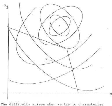
To show that i t is not merely curvature of the level curves that matters Figure 2-4 illustrates two quadratic functions - one can be considered a rotation of the other. One has the desired property of near-linearity over the feasible region while the other is distinctly nonlinear. Yet at a point such as x the curvature of the level curves is (by any measure) about the same for both functions.

Figure 2-4: Two constrasting cases of curvature

[image:51.561.117.505.287.656.2]