Abstract—The performance of the basic GPS system has been augmented by the technique of Differential GPS (DGPS) for military as well as civilian uses. Performance evaluation of a DGPS system requires the availability of DGPS corrections as functions of time. In many parts of the world, a lack of base stations and other infrastructure makes it impossible to have the desired quality and quantity of data. Thus, it is useful to develop a system, which can generate GPS measurements for an arbitrary number of truth points. In this paper, Wavelet Neural Network (WNN) is used to online predict the corrections for Selective Availability (S/A) on and off. Gradient Descent (GD) and Particle Swarm Optimization (PSO) are used to train and optimize the weights of WNN. Experimental results for the errors real-time prediction show the feasibility and effectiveness of WNN-PSO. The results prove that the proposed WNN-PSO method has better accuracy in a low cost GPS receiver.
Index Terms—Wavelet Neural Network, Prediction, Particle Swarm Optimization, Gradient Descent, DGPS.
I. INTRODUCTION
The overall quality of precise point positioning results is dependent on the quality of the Global Positioning System (GPS) measurements and user processing software. Dual frequency, geodetic-quality GPS receivers are routinely used both in static and kinematic applications for high accuracy point positioning. However, use of low-cost, single-frequency GPS receivers in similar applications creates a challenge because of how the ionosphere, multipath, and other measurement error sources are handled [1].
During past several years, the main problem in improving of the positioning measuring accuracy was Selective Availability (S/A) error. S/A was produced to degrade the achievable navigation accuracy when non-military single frequency GPS receivers are used. Although it is removed now, we investigated the system performance also under this limitation.
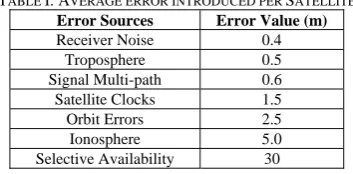
Other significant error sources for low cost receivers are signal delays from ionospheric and tropospheric effects, satellite clock drift, satellite orbital position errors, signal multi path, and noise generated within the receiver itself. Table I shows the common errors of GPS system in meters.
Manuscript received July 25, 2010.
Mohammad Divband is a student with the Computer Engineering Group, Iran University of Science and Technology, Behshahr, Iran (e-mail:
TABLE I. AVERAGE ERROR INTRODUCED PER SATELLITE Error Sources Error Value (m)
Receiver Noise 0.4
Troposphere 0.5 Signal Multi-path 0.6
Satellite Clocks 1.5
Orbit Errors 2.5
Ionosphere 5.0 Selective Availability 30
GPS accuracy can be improved over with Differential GPS (DGPS), where a reference station broadcasts corrections on common view satellites on a regular basis to the remote GPS receiver, which provides a corrected position output. A reference station calculates differential corrections for its own location and time then send the corrections to receivers, which are not far from it. Any interrupt of DGPS service will cause loss of navigation guidance, which has possibility of developing into a vehicle accident, particularly in the phase of precision approach and landing. Thus, achievement of corrections in any second is impossible for ordinary users [2].
There are two approaches to provide continuity performance of the DGPS corrections; one is to make the receivers hardware utilities more sophisticated and complicated. This solution could increase the accurate receivers cost. Consequently, non-military users would not benefit from low cost high–precision positioning. Another solution is to use software programs to improve the quality of positioning. In this paper, one of the soft computing techniques, improved Wavelet Neural Network, is used to predict the future corrections.
In order to improve the precision of the corrections forecasts, a Wavelet Neural Network (WNN) model, based on Particle Swarm Optimization (PSO), has been proposed. Corrections time series analysis requires mapping complex relationships between inputs and output, because the forecasted value is mapped as a function of patterns observed in the past. The DGPS corrections future value is represented by the previous data, as given in (1):
1
, 1
, ,
1
ˆ k F x k x k xk M
x (1)
Proposed method validity is verified with experiments on collected real data. This paper is organized as follow. Section II describes Wavelet Neural Network with GD learning rule. In section III, a brief introduction of PSO, then the proposed method for DGPS corrections prediction using WNN based on PSO will be described. In section IV, the experimental
A Comparison of Particle Swarm Optimization
and Gradient Descent in Training Wavelet
Neural Network to Predict DGPS Corrections
[image:1.595.338.515.221.308.2]results with real data are reported, before and after S/A error. Conclusions are presented in section V.
II. WAVELET NEURAL NETWORK STRUCTURE AND
GRADIENT DESCENT LEARNING METHOD
Recently, a new kind of Neural Networks known as the Wavelet Neural Networks (WNNs) have been proposed, which combine feed-forward neural network with the wavelet theory. It can provide better performance in function learning than conventional feed forward neural networks [3], [4].
A. Structure of WNN and Forward Calculation
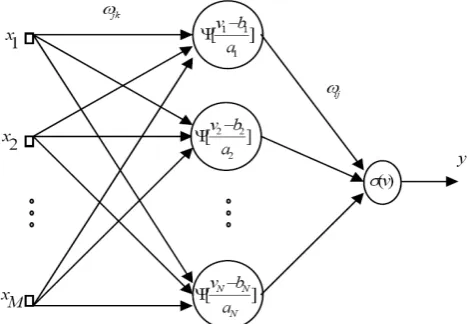
[image:2.595.49.284.309.471.2]This WNN consists of three layers: an input layer, a hidden layer, and an output layer. The input layer has M nodes. The output layer also has only one neuron whose output is the signal represented by the weighted sum of several wavelets. The hidden layer is composed of a finite number of wavelets representing the signal.
Fig. 1. Structure of a (M, N, 1) Wavelet Neural Network.
Consider a network consisting of a total of N neurons in hidden layer with M external input connections (Fig. 1). Let
x(n) denotes the M-by-1 external input vector applied to the network, y(n) denotes the output of the network, Wjk(n) presents the weight between the hidden unit j and input unit k,
Wij(n) denotes the connection weight between the output unit
i and hidden unit j, aj(n) and bj(n) present dilation and translation coefficients of wavlon in hidden layer at discrete time n, respectively.
The net internal activity of neuron j at time n, is given by:
M
xk
nK wjk n n
j 0
(2)
Where vj(n) is the sum of inputs to the j-th hidden neuron,
xk(n) is the k-th input at time n. The output of the j-th neuron is computed by passing vj(n) through the wavelets ψa,b j( ּ◌), obtaining: ] ) ( ) ( ) ( [ )] ( [
, a n
n b n v n v j j j j b a
(3)
The sum of inputs to the output neuron is obtained by:
)] ( [ ) ( ) ( , 0 n v n w n
v ab j
N j
ij
(4)
The output of the network is computed by passing vj(n) through the nonlinear function σ( ּ◌), obtaining:
)] ( [ )
(n v n
y (5)
B. Gradient Descent learning rule
GD learning rule is central to much current work on learning in artificial NN. GD provides a computationally efficient method of changing the weights in a feed forward network, with differentiable activation function units, to learn a training set of input-output examples.
The instantaneous sum of squared error at time n as:
2
2 [ ( ) ( )]
2 1 ) ( 2 1 )
(n e n y n d n
E (6)
Where d(n) denotes the desired response of output at time
n. To minimize of above cost function, the method of steepest descent is used. The weight between the hidden unit j and input unit k can be adjusted according to:
) ( ) ( ) ( )] ( [ , ) ( )] ( [ ) ( ) ( ) ( ) ( ) 1 ( n jk w n j a n k x n j v b a n ij w n v n e n jk w n jk w n E n jk w (7)
Where, η is a learning rate. The connection weight between the output unit i and hidden unit j is updated as follow: ) ( )] ( [ ) ( )] ( [ ) ( ) ( ) ( ) ( ) 1 (
, v n w n
n w n v n e n w n w n E n w ij j b a ij ij ij ij (8)
The translation coefficient of the j-th wavlon in hidden layer can be adjusted according to:
) ( ) ( 1 )] ( [ ) ( )] ( [ ) ( ) ( ) ( ) ( ) 1 ( , n b n a n v n w n v n e n b n b n E n b j j j b a ij j j j (9)
) ( ) ( ) ( ) ( )] ( [ ) ( )] ( [ ) ( ) ( ) ( ) ( ) 1 ( 2 , n a n a n b n v n v n w n v n e n a n a n E n a j j j j j b a ij j j j (10)
The wavelet function is “Gaussian-derivative” function as:
2
2 1
)
(x xe x
(11)
The usual sigmoid function of used in this research is as follow [5], [6]:
x e x 1 1 ) (
(12)
III. PARTICLE SWARM OPTIMIZATION AND TRAINING WNN
A. Introduction to PSO
Particle Swarm Optimization (PSO), first introduced by Kennedy and Eberhart in the mid 1990s. PSO employs a population of possible solutions to identify promising regions of the search space. The population is called swarm and the members of the population are called particles. Each particle represents a possible solution to the optimizing problem at hand. During an iteration of the PSO, each particle accelerates independently in the direction of its own personal best solution found so far, as well as the direction of the global best solution discovered so far by any other particle. Therefore, if a particle finds a promising new solution, all other particles will move closer to it, exploring the solution space more thoroughly [7].
A swarm consists of a set of particles moving around the search space, each representing a potential solution (fitness). Each particle has a position vector (ωi(t)), a velocity vector (vi(t)), the position at which the best fitness (pbesti) encountered by the particle, and the index of the best particle (gbest) in the swarm [8].
In each generation, the velocity of each particle is updated to their best-encountered position and the best position encountered by any particle using (13):
)) ( )( ( 2 2 )) ( )( ( 1 1 ) ( ) 1 ( t i gbest t r c t i i pbest t r c t i wv t i v (13)
The parameters c1 and c2 are called acceleration coefficients namely called self-cognitive and social parameter, respectively. r1(t) and r2(t) are random values, uniformly distributed between zero and one. The values of
r1(t) and r2(t) are not same for every iteration. w is called inertia weight and is employed to control the impact of the previous history of velocities on the current one. Shi and Eberhart [9] have found a significant improvement in the performance of PSO with the linearly decreasing inertia weight over the generations, time-varying inertia weight that
is given in (14):
2 2 1 ) max max ( ) ( w iter iter iter w w
w (14)
Where w1 and w2 represent the initial and final values of w, respectively, maxiter is the maximum number of optimization steps and iter represents the current iteration number. The position of each particle is updated every generation. This is done by adding the velocity vector to the position vector, as in (15):
) 1 ( ) ( ) 1
( t
i v t i t i
(15)
The algorithms output is the gbest particle, which contains final trained weights and thresholds.
IV. SIMULATIONS AND RESULTS
Computer simulation was performed to evaluate the correction prediction performance using WNN both with GD and PSO algorithms. The choice of the algorithms parameters is also very important. In this paper, the proposed methods parameters selection was based on the test data. The parameters of the proposed algorithms are listed in Table II.
TABLE II. PARAMETERS VALUES OF GD AND PSO
Algorithm Parameter name Parameter value
GD
Number of Training Epochs 7 Learning Factor Value 15
Momentum 0
PSO
Swarm Size 120
Self-recognition coefficient 2
Social coefficient 2
Inertia weight 0.9 → 0.4 Number of Iterations 50
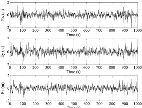
We tested both methods for one thousand times. Precise positioning needs X, Y, and Z, thus we executed the algorithms for these three time series. Fig. 2 to Fig. 5 show
[image:3.595.305.547.385.483.2]Ex, Ey, and Ez prediction errors (the difference between the predicted and real values) for 1000 test data.
[image:3.595.304.549.567.753.2]Fig. 3. 1000 Ex, Ey, and Ez prediction errors by using WNN-GD and S/A=on.
[image:4.595.41.289.36.687.2]Fig. 4. 1000 Ex, Ey, and Ez prediction errors by using WNN-PSO and S/A=off.
Fig. 5. 1000 Ex, Ey, and Ez prediction errors by using WNN-PSO and S/A=on.
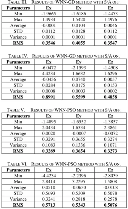
Six statistical measures (Min, Max, Average, Variance, Standard Deviation, and Root Mean Square) are used to evaluate prediction results for 1000 test data. Tables III to VI, show prediction errors statistical significance characteristics.
TABLE III. RESULTS OF WNN-GD METHOD WITH S/A OFF.
Parameters Ex Ey Ez
Min -1.9665 -1.6186 -1.4473
Max 1.4934 1.5420 1.4976
Average -0.0001 0.0104 0.0046
STD 0.0112 0.0128 0.0112
Variance 0.0001 0.0001 0.0001
RMS 0.3546 0.4055 0.3547
TABLE IV. RESULTS OF WNN-GD METHOD WITH S/A ON.
Parameters Ex Ey Ez
Min -6.0472 -2.1593 -1.4908
Max 4.4234 1.6632 1.6296
Average -0.0456 0.0740 0.0057
STD 0.0284 0.0175 0.0153
Variance 0.0008 0.0003 0.0002
RMS 0.8991 0.5599 0.4858
TABLE V. RESULTS OF WNN-PSO METHOD WITH S/A OFF.
Parameters Ex Ey Ez
Min -1.4895 -1.6552 -1.3857
Max 2.0434 1.6334 2.3861
Average 0.0020 -0.0007 -0.0072
STD 0.3291 0.3655 0.3274
Variance 0.1083 0.1336 0.1071
RMS 0.3289 0.3654 0.3273
TABLE VI. RESULTS OF WNN-PSO METHOD WITH S/A ON.
Parameters Ex Ey Ez
Min -4.4234 -2.2396 -2.8039
Max 2.8414 3.2295 1.5808
Average 0.0510 -0.0630 -0.0108
STD 0.5693 0.5309 0.5078
Variance 0.3241 0.2818 0.2578
RMS 0.5713 0.5343 0.5076
As shown in Tables III to VI, accuracy in Tables V and VI are higher than that in Tables III and IV. To clearly compare the results, total RMS errors are reported in Table VII.
TABLE VII. COMPARISON OF PREDICTION ACCURACY BY USING GD AND
PSO IN TRAINING WNN PREDICTOR.
Algorithm Total RMS error in S/A off
Total RMS error in S/A on
GD 0.6449 1.1654
PSO 0.5906 0.9324
V. CONCLUSION
[image:4.595.47.293.50.238.2] [image:4.595.318.535.52.406.2]REFERENCES
[1] T. Beran, D. Kim, and R. B. Langley, “High precision single-frequency GPS point positioning,” Proc. of ION GPS, 2003, pp. 1192-1200. [2] J. Sang, K. Kubik, and L. Zhang, “Prediction of DGPS Corrections
with Neural Networks,” Proc. of Intl. Conf. on Knowledge-Based
Intelligent Electronic Systems, Vol. 2, 1997, pp. 355-361.
[3] R. Drossu and Z. Obradovic, “Rapid Design of Neural Networks for Time Series Prediction,” IEEE Computational Sci. and Eng., No. 2, Vol. 3, 1996, pp. 78-89.
[4] Subanar and Suhartono, “New Procedures for Model Building in Wavelet Neural Networks for Forecasting non-Stationary Time Series,” Proc. of 5th Asian Mathematical Conf., Vol. 1, 2009, pp. 203-211.
[5] Y. Chen, B. Yang, and J. Dong, “Time-series prediction using a local linear wavelet neural network,” Neurocomputing, No. 6, Vol. 69, 2006, pp. 449-465.
[6] M. R. Mosavi, “A wavelet based neural network for DGPS corrections prediction,” WSEAS Trans. on Systems, 2004, pp. 3070-3075. [7] F. V. D. Bergh and A. P. Engelbrecht, “A Cooperative Approach to
Particle Swarm Optimization,” IEEE Trans. on Evolutionary
Computation, No. 3, Vol. 8, 2004, pp. 225-239.
[8] M. S. Arumugam, G. R. Murthy, M. V. C. Rao, and C. K. Loo, “A Novel Effective Particle Swarm Optimization Like Algorithm via Extrapolation Technique,” IEEE Conf. on Intelligent and Advanced Systems, 2007, pp. 516-521.