www.geosci-model-dev.net/10/1383/2017/ doi:10.5194/gmd-10-1383-2017
© Author(s) 2017. CC Attribution 3.0 License.
Climate SPHINX: evaluating the impact of resolution and stochastic
physics parameterisations in the EC-Earth global climate model
Paolo Davini1,2, Jost von Hardenberg3, Susanna Corti2, Hannah M. Christensen4,5, Stephan Juricke4, Aneesh Subramanian4, Peter A. G. Watson4, Antje Weisheimer4,6,7, and Tim N. Palmer4
1Laboratoire de Météorologie Dynamique/IPSL, Ecole Normale Supérieure, PSL Research University, CNRS, Paris, France 2Institute of Atmospheric Sciences and Climate (ISAC-CNR), Bologna, Italy
3Institute of Atmospheric Sciences and Climate (ISAC-CNR), Torino, Italy 4Atmospheric, Oceanic and Planetary Physics, University of Oxford, Oxford, UK 5National Center for Atmospheric Research (NCAR), Boulder, Colorado, USA 6National Centre for Atmospheric Science (NCAS), University of Oxford, Oxford, UK 7European Centre for Medium-Range Weather Forecasts (ECWMF), Reading, UK
Correspondence to:Paolo Davini ([email protected]) Received: 7 May 2016 – Discussion started: 23 June 2016
Revised: 17 February 2017 – Accepted: 26 February 2017 – Published: 31 March 2017
Abstract. The Climate SPHINX (Stochastic Physics HIgh resolutioN eXperiments) project is a comprehensive set of ensemble simulations aimed at evaluating the sensitivity of present and future climate to model resolution and stochas-tic parameterisation. The EC-Earth Earth system model is used to explore the impact of stochastic physics in a large ensemble of 30-year climate integrations at five different at-mospheric horizontal resolutions (from 125 up to 16 km). The project includes more than 120 simulations in both a historical scenario (1979–2008) and a climate change pro-jection (2039–2068), together with coupled transient runs (1850–2100). A total of 20.4 million core hours have been used, made available from a single year grant from PRACE (the Partnership for Advanced Computing in Europe), and close to 1.5 PB of output data have been produced on Super-MUC IBM Petascale System at the Leibniz Supercomputing Centre (LRZ) in Garching, Germany. About 140 TB of post-processed data are stored on the CINECA supercomputing centre archives and are freely accessible to the community thanks to an EUDAT data pilot project. This paper presents the technical and scientific set-up of the experiments, includ-ing the details on the forcinclud-ing used for the simulations per-formed, defining the SPHINX v1.0 protocol. In addition, an overview of preliminary results is given. An improvement in the simulation of Euro-Atlantic atmospheric blocking fol-lowing resolution increase is observed. It is also shown that
including stochastic parameterisation in the low-resolution runs helps to improve some aspects of the tropical climate – specifically the Madden–Julian Oscillation and the tropi-cal rainfall variability. These findings show the importance of representing the impact of small-scale processes on the large-scale climate variability either explicitly (with high-resolution simulations) or stochastically (in low-high-resolution simulations).
1 Introduction
of 16–40 km, whereas the resolution of CMIP5 climate mod-els is (on average) coarser than 120 km.
It is well known that a typical climate model is un-able to represent many sub-synoptic-scale systems, and only poorly represents smaller baroclinic features. Typically cli-mate models underesticli-mate the number of observed storms (Zappa et al., 2013) and poorly simulate the statistics of atmospheric mid-latitude blocking (Davini and D’Andrea, 2016). In fact it has been shown (e.g. van Oldenborgh et al., 2012) that at standard (low) climate resolution, forecast sys-tems have pervasive systematic errors, which impact on quasi-persistent weather regimes (Dawson et al., 2012) and, more generally, on temporal variability and regional patterns of the leading modes of variability (Delworth et al., 2012; Kinter III et al., 2013). On the other hand, recent experiments have shown that high-resolution climate models are signifi-cantly better at simulating important physical processes, such as the global water cycle (Demory et al., 2014), as well as rel-evant features of the large-scale atmospheric circulation such as the jet stream (Lu et al., 2015), the Euro-Atlantic blocking (Jung et al., 2012) and the Madden–Julian Oscillation (MJO; Peatman et al., 2015).
The fact that enhanced horizontal resolution in climate models can positively impact some aspects of the simulated large-scale atmospheric circulation is further evidence of the role that small-scale processes play in “shaping” large-scale motions. However, it is unlikely that climate integrations at very high resolution (i.e. at the resolution used in NWP), will be feasible in the near future. There are numerous other areas of climate model development that compete for the given computing resources, e.g. the need for ensembles of integrations, the need to integrate over century and longer timescales, and the need to incorporate additional Earth sys-tem complexity. In addition, parameterisations, which have been developed for coarse scales, may need retuning or to be replaced with alternative parameterisations at higher resolu-tions, which require a consistent development effort.
Instead of explicitly resolving small-scale processes by in-creasing the resolution of climate models, a possible alterna-tive is to use stochastic parameterisation schemes. There has been significant progress in developing stochastic schemes over the last decade, primarily for use in medium-range and seasonal ensemble forecasts (e.g. Plant and Craig, 2008; Khouider et al., 2010; Bengtsson et al., 2013; Grell and Fre-itas, 2013; Dorrestijn et al., 2016; Sakradzija et al., 2016; Ollinaho et al., 2016). These schemes introduce an element of randomness into physical parameterisation schemes to ac-count for the impact of uncertain, unresolved processes on the resolved-scale flow (Palmer, 2012). Stochastic schemes have been shown to improve the reliability of probabilistic forecasts on medium-range and seasonal timescales, as well as improving biases in the mean state.
There is mounting evidence that stochastic parameterisa-tions can also prove beneficial for climate simulaparameterisa-tions (e.g. Lin and Neelin, 2000, 2003; Arnold et al., 2013). Berner et al.
(2012) showed that including stochastic physics can reduce systematic biases in the model’s mean climate, comparable to improvements gained by increasing the model resolution. Several recent papers have also demonstrated that the vari-ability of a climate model can significantly improve with the introduction of a stochastic physics scheme, with improve-ments observed in the representation of the MJO (Deng et al., 2015; Wang et al., 2016), the El Niño–Southern Oscillation (Christensen et al., 2017a) and extra-tropical flow regimes (Weisheimer et al., 2014; Dawson and Palmer, 2015; Chris-tensen et al., 2015). As was the case for the mean state, the observed improvements can be similar to that observed on increasing the resolution of the model (Dawson et al., 2012). These results highlight the influence of small-scale pro-cesses on large-scale climate variability, and indicate that al-though simulating variability at small scales is a necessity, it may not be necessary to represent the small scales accu-rately, or even explicitly, in order to improve the simulation of large-scale climate. This issue is important in light of the next CMIP6 project. In fact, it seems quite unrealistic that in the near future climate simulations at NWP resolution could be affordable. However, resolutions around 40 km might be more feasible and indeed they are planned within the High-ResMIP project (Haarsma et al., 2016).
In the coordinated project Climate SPHINX (Stochas-tic Physics HIgh resolutioN eXperiments), we use the EC-Earth EC-Earth system model (Hazeleger et al., 2010, 2012, http://www.ec-earth.org) to investigate the sensitivity of cli-mate simulations to model resolution and stochastic parame-terisations. A key aim of the study is to investigate the degree to which stochastic parameterisation schemes can be used as a computationally cheaper alternative to increased model res-olution.
is a true passing threshold in resolution, which is required to get acceptable simulations of the main climate features.
By comparing integrations carried out at different resolu-tions, we evaluate the impact of increased atmospheric hori-zontal resolution on the simulation of key climate processes and of climate variability. By comparing experiments with and without the implementation of stochastic physics, we evaluate the impact of stochastic physics on the simulation of key climate process and of the associated climate vari-ability when the model resolution is the same. By comparing experiments with the implementation of stochastic physics with experiments carried out without stochastic physics, but at higher resolutions, we assess to what extent the stochastic representation of the sub-grid processes can compete with a more refined horizontal resolution. The results of this project integrate with several other efforts currently underway (e.g. the European Union’s Horizon 2020 PRIMAVERA project, https://www.primavera-h2020.eu/). In particular this study complements groundbreaking past initiatives in pioneering the use of HPC (high-performance Computing) for climate simulations such as the UPSCALE (Mizielinski et al., 2014) and the ATHENA (Kinter III et al., 2013) projects.
Climate SPHINX was made possible by a considerable amount of computing time provided by PRACE (the Part-nership for Advanced Computing in Europe) and data stor-age from EUDAT (the collaborative pan-European infras-tructure providing research data services). We were granted 20 million core hours during a single year at SuperMUC, the IBM Petascale System at the Leibniz Supercomputing Centre (LRZ) in Garching near Munich, Germany. Storage of data produced by Climate SPHINX is secured by the EUDAT pi-lot project DATA SPHINX (DATA Storage and Preservation of High-resolution climate eXperiments), which provides a widely accessible archive for medium-term storage to facili-tate data access and discovery. DATA SPHINX is managed by CINECA (the largest Italian computing centre) and at present hosts 140 TB of data generated by Climate SPHINX. In this paper we describe in detail the important techni-cal aspects of this project and highlight some preliminary scientific results on the impact of increased resolution and stochastic parameterisations on climate simulations. Model configuration and tuning are presented in Sect. 2, while the experimental set-up is described in Sect. 3. Section 4 is de-voted to detail the technical configuration. An overview of results and concluding remarks are reported in Sects. 5 and 6, which is followed by the “Data availability” section.
2 The EC-Earth global climate model
In Climate SPHINX, version 3.1 of the state-of-the-art EC-Earth atmosphere–ocean EC-Earth system model (Hazeleger et al., 2010, 2012) has been used.
The atmospheric component of EC-Earth is based on cy-cle 36r4 of the Integrated Forecast System (IFS)
circula-tion model (ECWMF, 2009), which has been developed by the European Centre for Medium-Range Weather Forecasts (ECMWF). This has been tuned and improved for climate purposes by the EC-Earth consortium. IFS uses a combina-tion of spectral and reduced Gaussian grids (where, in the latter, the number of longitudinal grid points decreases to-wards the poles). Physical parameterisations and advection are computed on the reduced Gaussian grid and then, us-ing the spectral transform, semi-implicit time steppus-ing is per-formed in the spectral space.
Traditionally, the spectral harmonic at which truncation occurs defines the horizontal resolution; IFS uses a linear tri-angular truncation for which a specified number of N har-monics retained corresponds to 2(N+1)grid points along the Equator. If the resolution is T255, this means that post-processed output will have 512×256 grid points on a regu-lar Gaussian grid, which corresponds to a resolution of about 80 km at the Equator. The description of the main parame-terisation schemes within IFS can be found in Beljaars et al. (2004); the parameterisations are in general independent of resolution, with the only exception of the convective adjust-ment time, which decreases with increasing resolution as re-ported in Table 1.
To represent land-surface dynamics, IFS integrates the Hydrology Tiled ECMWF Scheme of Surface Exchanges over Land (H-TESSEL) land-surface scheme (Balsamo et al., 2009). When used in coupled mode, the Nucleus for Euro-pean Modelling of the Ocean (NEMO) version 3.3.1 oceanic circulation model (Madec, 2008) is used; this makes use of a tripolar grid with the poles placed over northern Siberia, North America and Antarctica. NEMO includes the Lou-vain la Neuve (LIM) sea ice model version 3 (Vancoppenolle et al., 2012). The atmospheric and oceanic components are coupled through OASIS3 (Valcke, 2013), with a coupling frequency of 3 h.
2.1 The stochastic physics parameterisation schemes
We consider two complementary approaches to stochas-tic parameterisation, both developed at ECMWF for IFS. The two schemes considered here are used operationally at weather and seasonal forecasting centres worldwide (Palmer et al., 2009; Yonehara and Ujiie, 2011; Bouttier et al., 2012; Sanchez et al., 2016), and so have been extensively tested in a range of models on medium range and seasonal timescales. Following the “seamless prediction” paradigm, we choose to test these schemes here on climate timescales.
Table 1.Resolution-dependent scientific configuration for EC-Earth in the Climate SPHINX experiments. The same number of ensemble members has been run for present-day AMIP (PDA) and future scenario AMIP (FSA) experiments. T255C is the coupled configuration used for past-to-future coupled (PFC) simulations. Resolution is estimated at the Equator. The number of members indicate the deterministic and stochastic members. Backscatter ratio (tuning parameter for SKEB stochastic scheme), convective adjustment time (tuning parameter for deep convection) and momentum launch (tuning parameter for non-orographic gravity waves) are unitless.
Truncation Resolution No. of members Time step Backscatter ratio Conv. adj. time Mom. launch
T159 125.2 km 10+10 3600 s 0.032 2.6 0.00375
T255 78.3 km 10+10 2700 s 0.040 2.0 0.00375
T511 39.1 km 6+6 900 s 0.085 1.5 0.00375
T799 25.0 km 3+3 720 s 0.095 1.3 0.00368
T1279 15.7 km 1+1 600 s 0.095 1.2 0.00334
T255C 78.3 km 3+3 2700 s 0.040 2.0 0.00375
Shutts and Pallarès, 2014). SPPT can be expressed as
∂X
∂t =D+K+(1+µe) X
i
Pi, (1)
where ∂X∂t is the modelled total tendency inX. This is the sum ofD, the dynamical tendency,K, the horizontal diffu-sion, and eachPi term, withPi being the tendency from the ith physics scheme. The zero mean random perturbation,e, is constant in the vertical, but µ tapers the perturbation to zero close to the surface and in the stratosphere. The scheme acts on the tendencies of the physical fields (i.e. temperature, winds and specific humidity) resulting from the five main parameterisation schemes: radiation, turbulence and gravity wave drag, non-orographic gravity wave drag, convection, and large-scale water processes. All variables are perturbed with the same random number.
The perturbation, e, is generated using a spectral pattern generator (Berner et al., 2009), ensuring that it smoothly varies in space, while the patterns evolve in time follow-ing an AR(1) process. The perturbation at each time step is the sum of three independent random fields, which represent uncertainties on different temporal and spatial scales. The fields have horizontal correlations of 500, 1000 and 2000 km and temporal decorrelations of 6 h, 3 days and 30 days re-spectively, with associated standard deviations of 0.52, 0.18 and 0.06. The magnitude of the perturbation has been mo-tivated through coarse-graining high-resolution model sim-ulations (Shutts and Pallarès, 2014), and a recent coarse-graining study has also provided justification for the noise temporal and spatial correlation scales (Christensen et al., 2017b). While the smallest scale (500 km and 6 h) domi-nates on weather forecasting timescales, it is expected that the larger scales will also be important on climate timescales. The SPPT scheme requires no retuning with changing hori-zontal resolution: the same noise characteristics are used op-erationally at ECMWF across model resolutions. This is be-cause the multiplicative nature of the scheme applied to the total of all parameterised physical tendencies results in per-turbations to the model that scale automatically as the
pa-rameterised tendencies scale with resolution. The resolution dependence of the individual contributions from the parame-terisation schemes is implicitly dealt with at the (determinis-tic) parameterisation level.
In contrast to SPPT, the SKEB scheme aims to represent a physical process that is otherwise absent from the model (Shutts, 2005; Palmer et al., 2009). Kinetic energy loss is common in models due to numerical integration schemes and the parameterisation process (Berner et al., 2009). To coun-teract this, the SKEB scheme represents upscale transfer of kinetic energy by randomly perturbing the stream function.
Similar to SPPT, the SKEB scheme uses a spectral pattern generator to generate a spatially and temporally correlated perturbation field, which is added at each time step to the deterministic stream function tendency,
˙
ψt(φ, λ, t )=ψ˙det(φ, λ, t )+f (φ, λ, t ), (2) whereψ˙
tis the total stream function tendency,ψ˙detis the de-terministic tendency andf is the additive perturbation field. The perturbation field is expressed in spherical harmonics, and each coefficient is evolved separately in time following an AR(1) process. A tuning parameter for the SKEB scheme, the backscatter ratio, is set to increase following resolution increase (see Table 1; following practice at ECMWF) in or-der to improve the slope of the kinetic energy spectrum.
which is now equal to that in the run where the SPPT scheme is disabled. This fix has subsequently been implemented at ECMWF (Leutbecher et al., 2017).
Hereafter, Climate SPHINX simulations where stochastic parameterisation is operational will be defined as “stochas-tic” runs, while simulations where the scheme is deactivated will be mentioned as “deterministic” runs.
2.2 Model tuning
With respect to the previous version (v3.0.1), EC-Earth 3.1 shows a reduced radiative imbalance and an improved hydro-logical cycle (Davini et al., 2014). However, it still exhibits a cold bias in both its atmosphere-only and coupled config-uration and a small imbalance inP −E. In a “present day” AMIP configuration, the 3.1 version is too cold, extracting heat from the underlying sea surface temperatures (SSTs) by about 1.5 W m−2and showing unrealistically high values for net SW (shortwave) and LW (longwave) fluxes at TOA (top of the atmosphere) (around 243–244 W m−2). Thus, the first goal of the tuning was to provide reasonable radiative fluxes at TOA and at the surface for the standard deterministic ver-sion of the model (T255; see next paragraph for further de-scription on the configurations adopted).
To improve the radiation budget, some of the convection and microphysical parameters from a more recent version of IFS (cy40r1) were retrieved. In addition to this, two standard tuning parameters have been modified (see Mauritsen et al., 2012); the entrainment rate for organised convection (EN-TRORG) was reduced from 1.75×10⁻⁴to 1.5×10⁻⁴, and the rate of conversion of liquid water to rain (RPRCON) was reduced from 1.4×10⁻³to 1.2×10⁻³.
The optimal choice of tuning parameters provides reason-able fluxes at the TOA (around 240 W m−2) and a positive flux at the surface of about 0.6 W m−2, in accordance with the best estimates from observations (Wild et al., 2013). It is im-portant to note that the tuning of the radiative fluxes has been carried out only for the T255 deterministic model version: the radiative balance has not been tuned in the higher res-olution or stochastic models. This ensures a clean compari-son between simulations at different resolutions and with and without stochastic physics. If the model were re-tuned for each run, it is not possible to determine whether it is chang-ing the tunchang-ing parameters, changchang-ing the resolution or includ-ing stochastic physics that are responsible (Haarsma et al., 2016). Including the SPPT scheme led to a negative bias in the surface heat fluxes of about 0.8 W m−2, likely caused by a different distribution of the clouds.
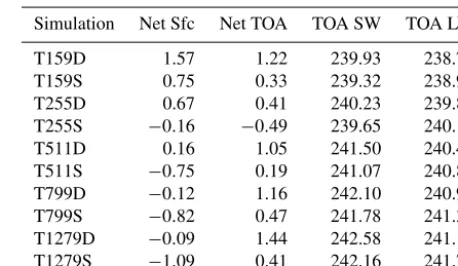
The main radiative fluxes resulting after the complete tun-ing procedure are reported in Table 2. As shown in this table, the radiative balance of the model at higher resolution (and with stochastic physics) shows larger TOA SW and LW with increasing resolution. Net surface fluxes are highly variable, with higher values for coarser resolutions.
Table 2.Radiative fluxes expressed in W m−2for the reference ex-periment (i.e. the first simulation run) at different resolution for present-day AMIP (PDA) simulations. D stands for deterministic simulation, S for stochastic. Fluxes have been tuned for T255D.
Simulation Net Sfc Net TOA TOA SW TOA LW
T159D 1.57 1.22 239.93 238.71
T159S 0.75 0.33 239.32 238.99
T255D 0.67 0.41 240.23 239.82
T255S −0.16 −0.49 239.65 240.14
T511D 0.16 1.05 241.50 240.44
T511S −0.75 0.19 241.07 240.88
T799D −0.12 1.16 242.10 240.94
T799S −0.82 0.47 241.78 241.31
T1279D −0.09 1.44 242.58 241.14
T1279S −1.09 0.41 242.16 241.74
Sfc: surface; TOA: top of the atmosphere; SW: shortwave; LW: longwave.
Finally, a supplementary modification – derived from a more recent IFS cycle – has been performed in order to pro-duce a realistic quasi-biennial oscillation (QBO) at all res-olutions. The EC-Earth 3.1 non-orographic gravity waves scheme is characterised by a momentum flux that is con-tinuously launched in the mid-troposphere to simulate the effect of gravity waves. The latitudinal profile of this mo-mentum flux governs the correct parameterisation of gravity waves: a too high amplitude of the momentum flux will dis-turb the QBO in equatorial zones, particularly at high reso-lutions, while a too low value will lead to unrealistic eddy-driven jets, especially in the Southern Hemisphere, where orographically induced wave drag is low. With the current latitudinal profile, the QBO was simulated only at standard resolution (T255 with 91 vertical levels). Following advice from ECMWF staff, a resolution-dependent parameterisation of non-orographic gravity wave drag replaced the version-dependent parameterisation present in EC-Earth 3.1 (an ad hoc parameterisation developed for the ECMWF System 4 seasonal forecast system). Namely, instead of using a low-momentum flux average value (GFLUXLAUN=0.02) with a positive Gaussian peak at 50◦S, we use a higher value
(GFLUXLAUN=0.0375), which is reduced with a Gaussian shape at the Equator. This negative peak is slightly deeper for stochastic runs than for deterministic simulations to compen-sate for the effect of the stochastic noise. The average value of the momentum flux was further reduced with increasing resolution (starting from T799) according to the ECMWF specification for IFS cy40r1 (see Table 1).
3 Science configuration: the SPHINX v1.0 protocol The following sections describe the scientific configuration, including the simulations performed, the initial and boundary conditions, the SST and sea ice concentration (SIC) used that together define the SPHINX v1.0 protocol.
3.1 Climate SPHINX simulations
Climate SPHINX simulations are grouped into three main blocks: present-day AMIP (PDA), future scenario AMIP (FSA) and past-to-future coupled (PFC). PDA and FSA are atmosphere-only simulations: 20 ensemble members are run at T159 (∼125 km), 20 at T255 (∼80 km), 12 at T511 (∼40 km), 6 at T799 (∼25 km) and 2 at T1279 (∼16 km) for both PDA and FSA experiments. For each resolution, half of the ensemble members have the stochastic physics param-eterisations activated. All simulations have the same vertical grid with 91 levels (L91): these are hybrid levels with the last full level at 0.01 hPa. The number of ensemble members run and their resolution are also reported in Table 1.
The atmosphere-only experiments extend for 30 consecu-tive years, from 1979 to 2008 for PDA, while FSA experi-ments are run from 2039 to 2068.
PFC simulations are run with IFS at the T255L91 configu-ration, coupled with NEMO using the ORCA1 grid (a tripo-lar grid with resolution of 1◦longitudinally and refinement to 1/3◦at the Equator) with 46 vertical levels. The upper model level is at ca. 3 m and 10 levels are in the upper 100 m. Six ensemble members are run, three with the stochastic parame-terisation active and three control members without stochas-tic parameterisation, from 1850 to 2100.
3.2 Initial conditions
The initial conditions (ICs) in both the PDA and FSA exper-iments are taken from the ECMWF ERA-Interim Reanalysis (Dee et al., 2011) for 1 January 1979. A first experiment is run at each resolution for a few days, and it is used to cre-ate the ICs for the other experiments. For instance, for T255 experiments, the ICs for the 10 ensemble members are ex-tracted using the midnight values (00:00) from each of the first 10 days respectively, and then reassigned to 1 January.
The same ICs are used also for FSA: in order to account for the land-surface adjustment to the new forcing, a 1-year spin-up has been carried out for FSA (which is therefore starting from 2038).
For PFC simulations, given the different expected clima-tologies of integrations with/without stochastic physics, two 320-year spin-ups are carried out in coupled mode to equili-brate the ocean to the atmospheric forcing. Having spun-up, three oceanic states – from spin-up year 300, 310 and 320 – are coupled with three different atmospheric ICs; these are run in coupled mode for a further 10 years with fixed green-house gas (GHG) forcing for the year 1850. In this way the
phase space distance between the simulations is 20 years and the atmosphere and land surface have had enough time to ad-just to the new oceanic state.
3.3 Forcing and boundary conditions
Well-mixed GHGs, stratospheric ozone and volcanic aerosol concentrations have been set according to the CMIP5 proto-col (Moss et al., 2010; Taylor et al., 2012). Historical forc-ing is used for PDA experiments, whereas for the FSA ex-periments the high emission scenario (Representative Con-centration Pathway 8.5, RCP8.5) is adopted. PFC simula-tions use the historical CMIP5 specification from year 1850 to year 2005 included; after that, the forcing is taken from the RCP8.5 scenario. Albedo, land use and vegetation pat-terns are set using the standard configuration of EC-Earth 3.1, which uses a MODIS-derived fixed climatological sea-sonal cycle for snow-free albedo and the leaf area index. The average yearly solar irradiance was set at 1368.2 W m−2with intrannual variations, following the standard EC-Earth 3.1 set-up. All the simulations of PDA and FSA experiments use this set-up. For the PFC simulations interannual variations following CMIP5 prescriptions (i.e. the 11-year solar cycle) have been added.
3.4 Present-day SST and SIC
Given that both FSA and PDA simulations are atmosphere-only runs, a special effort has been taken to provide reliable SSTs in order to fully exploit the high resolution.
For PDA, SSTs have been obtained from the daily SST and SIC HadISST2.1.1, a pentad-based dataset with a resolution of 0.25◦×0.25◦for SSTs (Kennedy et al., 2017) and 1◦×1◦
for SIC (Titchner and Rayner, 2014). These are bilinearly interpolated onto the required reduced Gaussian grid for each resolution: climatologies for SST and SIC for the 1979–2008 period can be seen in the upper panels of Fig. 1.
A number of inconsistencies are found between the land– sea mask of IFS and of HadISST2.1.1; these are due to slightly different coastlines and a different representation of the lakes. For the different coastlines, linear extrapolation from HadISST2.1.1 has been performed. For the interior (i.e. lakes), a methodology similar to the one used in ERA20CM dataset (Hersbach et al., 2015) has been adopted: 1-month lagged 2 m temperatures from the ERA-Interim monthly cli-matology of 1979–2008 are used as SST. Where the tem-perature is below zero, SIC is set to one, otherwise it is left at zero. This is interpolated in time on a daily basis and in space on the needed grid to create a smoothed seasonal cycle for lakes.
3.5 Future scenario SST and SIC
Figure 1. (a, b)HadISST 2.1.1 climatology for the SSTs(a)and SIC(b)for the 1979–2008 period.(c, d)Climatological changes between the FutureHadISST 2.1.1 dataset and the HadISST 2.1.1 dataset for SST(c)and SIC(d).
state-of-the-art global coupled models (i.e. the CMIP5 mod-els). However, the oceanic component of these models has generally a low horizontal (of the order of 1◦) and temporal
(usually monthly) resolution, in which the oceanic circula-tion is not perfectly resolved. In order to improve our bound-ary conditions, we decided to take advantage of the high tem-poral and spatial resolution provided by the HadISST2.1.1. As a consequence, the SST for FSA experiments have been obtained as a combination of HadISST2.1.1 variability and the CMIP5 EC-Earth simulations ensemble mean trend.
First, the 1979–2008 HadISST2.1.1 SST has been de-trended point by point to provide a set of anomalies with realistic variability. Second, the monthly seasonal cycle of the difference between the CMIP5 EC-Earth RCP8.5 ensem-ble mean over 2038–2068 (10 members) and the CMIP5 EC-Earth historical ensemble mean over 1979–2008 (10 mem-bers) has been computed. This provides for each grid point the average expected SST increase from the present-day to the future period according to a GCM (Global Circulation Model), as a function of calendar month. To account for changes in SST during the FSA period, for each grid point the average trend in SST from the CMIP5 EC-Earth RCP8.5 integrations for 2038–2068 was also extracted. All CMIP5 EC-Earth data were bilinearly interpolated in space on the HadISST2.1.1 grid and linearly in time to daily frequency.
Finally, a new Step1HadISST dataset has been created combining the detrended HadISST2.1.1 (expressing the high-resolution daily variability), the average daily change of CMIP5 EC-Earth (from RCP8.5 and historical,
express-ing the expected average temperature increase) and the lin-ear trend of the CMIP5 EC-Earth RCP 8.5 (expressing the expected future trend in SST). The methodology used here, which shares the main characteristics with the method devel-oped by Mizuta et al. (2008), is sketched in Fig. 2.
However, the Step1HadISST reconstruction misses an im-portant element; there is no information on the sea ice cover in the future. To account for this, we took data from the CMIP5 EC-Earth simulations as a reference for SIC. CMIP5 EC-Earth simulations show a considerable cold bias in SST with respect to HadISST2.1.1, but they show good sea ice coverage, especially for the Northern Hemisphere (see aver-age Northern Hemisphere and Southern Hemisphere SIC in Fig. 3).
Considering that an ensemble mean would be unrealistic, especially for a field with a large spatial variance as sea ice, we select a single ensemble member representative of the en-semble. Member “r8i1p1” has been chosen to characterise the ensemble, since its climatology shows the smallest SIC root mean square error (RMSE) when compared to the en-semble mean climatology in the time window 2038–2068. Clearly, using RMSE is only one of the possible metric to perform such selection; our main goal is to pick an ensem-ble member that is not an outlier when compared to the other EC-Earth CMIP5 ensemble members.
HadISST2.1.1 EC-Earth RCP8.5
EC-Earth historical
1979 2008 2039 2068
2039 2068
FutureHadISST2.1.1 EC-Earth
mean change
Detrended HadISST2.1.1
EC-Earth RCP8.5 trend
Figure 2. Scheme representing the methodology adopted to cre-ate the FutureHadISST 2.1.1. The new dataset is a combination of detrended daily variability from HadISST 2.1.1, CMIP5 EC-Earth mean change and CMIP5 EC-Earth RCP8.5 trend.
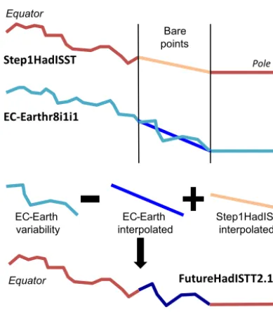
above. We define these as “bare point”. For bare points, we want to make use of the model variability, but we do not want to have inconsistent SST at the boundaries (i.e. where bare points border the Step1Hadisst dataset).
Initially, we perform a linear extrapolation for bare points for Step1HadISST SSTs – which gives us a measure of the average SSTs at the bare points. However, these extrapo-lated values are missing a realistic spatial variability. We then mask the bare points also in the SST field of the CMIP5 EC-Earth ensemble member “r8i1p1”, and we subsequently lin-early extrapolate new values. We then subtract from the orig-inal field of CMIP5 EC-Earth ensemble member “r8i1p1” these new extrapolated values, in order to obtain an anomaly field, which includes the spatial and temporal variability of the SST field over the bare points given by CMIP5 EC-Earth “r8i1p1”. This final field is then added to the linearly extrap-olated Step1HadISST SST.
Hence, for each day, the SSTs for bare points are given by the EC-Earth CMIP5 RCP8.5 ensemble member “r8i1p1” SST minus extrapolated EC-Earth CMIP5 RCP8.5 SSTs plus extrapolated Step1HadISST. The methodology to obtain this specific SST reconstruction is illustrated in Fig. 4.
This provides a pattern of SSTs physically consistent with SICs; indeed, it avoids unrealistic values of SSTs in the prox-imity of the polar cap during winter and – using the CMIP5 EC-Earth data – it provides a reasonable distribution of SSTs in summer, where in the future scenario the sea ice cover-age in the Northern Hemisphere often disappears. Moreover, there is no discontinuity at the border with Step1HadISST. The new dataset is defined as FutureHadISST2.1.1.
The same methodology used for the PDA simulations has been adopted also for FSA runs in order to solve the is-sues of the lakes and the different land sea mask; however, in this case we must account for the estimated temperature change over land. We consider the difference between the 1-month lagged 2 m surface temperature from CMIP5 EC-Earth RCP8.5 and the 1-month lagged 2 m surface temper-ature from CMIP5 EC-Earth historical ensemble (averaged over eight members). We then add this to the 1-month lagged 2 m surface temperature ERA-Interim monthly climatology of 1979–2008. This, analogous to what was done for SSTs, accounts for climate change.
The SST and SIC changes between FutureHadISST2.1.1 and HadISST2.1.1 are reported in Fig. 1; as expected larger warming and sea ice retreat is seen in the Northern Hemi-sphere high latitudes. Figure 3 reports the time series and trends for SST (between 45◦S and 45◦N) and SIC (for
both Northern and Southern hemispheres) for both Future-HadISST2.1.1 and Future-HadISST2.1.1.
4 Technical configuration
4.1 High-performance computing details
Simulations have been run on the 6.8 PFLOP SuperMUC IBM Petascale System at LRZ. The initial set-up and config-urations have been performed on the Supermuc-I platform, based on Sandy Bridge-EP Xeon E5-2680 8C processors. For processor decomposition the Message Passage Interface (MPI) parallelism paradigm has been used. EC-Earth allows also for OpenMP/Shared memory parallelisation, which has been tested without showing any significant computational benefit.
An accurate scaling of the performance was performed during the first months of the simulations. However, a conser-vative choice has been undertaken, after considering that the wall time needed to run the simulations was not the main con-cern for the project success. The number of cores assigned to each experiments have been selected following the resolution of the model considered. Although stochastic physics exper-iments showed about 5–10 % decrease in performance (ac-cording to different resolutions), the same number of cores has been retained.
In summer 2015, a new Supermuc-II platform based on Haswell Xeon E5-2697 v3 processors was made available by the LRZ. The new HPC granted a reduction of about 5 % of the total core hours used, without affecting the wall time. About 75 % of the simulations have been run using the Haswell nodes. Details on the processor decomposition, computational costs and data outputs are reported in Table 3. 4.2 Data output and post-processing
simu-Figure 3. (a)Time series for 45◦S–45◦N yearly averaged SST for present-day HadISST 2.1.1 (red), FutureHadISST 2.1.1 (violet) and CMIP5 EC-Earth ensemble mean (light blue).(b)Time series for Northern Hemisphere (filled circles) and Southern Hemisphere (empty circles) yearly averaged sea ice area for HadISST 2.1.1 (dark blue), FutureHadISST 2.1.1 (green), CMIP5 EC-Earth ensemble member “r8i1p1” (light blue) and the CMIP5 EC-Earth ensemble mean (faint blue).
Table 3.Resolution-dependent technical details for EC-Earth in the Climate SPHINX experiments. T255C is the coupled configuration used for PFC simulations. Wall time has been measured on the Supermuc-II Haswell platform, and it is evaluated for deterministic simulations; stochastic simulations wall time is about the 5 % higher.
Truncation No. of cores Wall time (per year) Leg length Output data (per year) Post-proc data (per year)
T159 224 52 min 1 year 26 GB 9.7 GB
T255 588 1 h 12 min 1 year 64 GB 24 GB
T511 840 6 h 10 min 6 months 249 GB 35 GB
T799 1120 14 h 2 months 605 GB 57 GB
T1279 1540 30 h 1 month 1.6 TB 111 GB
T255C 588 1 h 35 min 1 year 38 GB 30 GB
lations alone sum up to about 200 TB of raw data output. Summing together the restarts files and the output of all ex-periments the total amount of space occupied at the peak of the project (February 2016) reached about 1 PB. In order to reduce the size of the output and to increase the data acces-sibility to a larger audience, automatic post-processing rou-tines have been implemented. At the end of each simulation leg, a script aimed at post-processing is launched; the script handles both the spectral and reduced Gaussian data from IFS and extracts and converts the requested variables from the default ECMWF format to a user-friendly, CMOR-like format on regular Gaussian grid. With this automatic pro-cedure, more than 140 TB of post-processed data has been
produced. A significant reduction of the data volume was ob-tained making use of the NetCDF-4 Zip format.
radia-Step1HadISST
EC-Earthr8i1i1
Bare points
Pole Equator
FutureHadISTT2.1.1 EC-Earth
variability
EC-Earth interpolated
Step1HadISST interpolated
Pole Equator
Figure 4.Scheme representing the methodology adopted to fill the “bare points”, i.e. the points where sea ice has retreated in the CMIP5 EC-Earth RCP8.5 simulation. Each line represent a SST profile from the Equator to the pole.
tive variables (SMON). A few fields that are non-linear func-tions of the output (e.g. specific humidity) have been com-puted from the original 3 h output and then averaged at the required frequency in order to record them accurately. In ad-dition to the atmospheric data, about 10 TB of oceanic output has been stored for PFC simulations. Data at daily and pentad frequency have been retained.
All the data, including raw output, post-processed data and restart files, have been archived on the tape archives of the Tivoli Storage Management Infrastructure of the LRZ.
5 Results overview
In this section we present a brief overview of the preliminary findings of the Climate SPHINX project. Considering that the number of diverse climate aspects that could be analysed in such a large dataset is large, we decided to present here-after only a few selected features of the mean climate and its variability. For all the results presented – if not specified dif-ferently – the complete set of ensemble members available for the present-day climate (i.e. PDA experiments) has been used.
5.1 Mean climate
Although a detailed analysis of the mean climate in all the simulations performed would be excessively long to be in-cluded in the present work, we introduce a couple of figures showing the sensitivity to resolution and stochastic physics parameterisation of the climatology of precipitation (Fig. 5)
and 200 hPa zonal wind (Fig. 6). We compare the ensemble mean average fields of a low-resolution version (T255) with a high-resolution one (T799), in both its deterministic and stochastic configurations. Data have been interpolated on a common 2.5◦×2.5◦grid.
The precipitation model bias – shown in Fig. 5, with re-spect to Global Precipitation Climatology Project (GPCP) dataset (Huffman et al., 2001) – is especially strong in Indian Monsoon region, with an excess of precipitation from the In-dian Ocean to the western Pacific. More generally, EC-Earth tends to underestimate the precipitation over the continents and overestimate it over the oceans. When the comparison is carried out between stochastic and deterministic config-urations, it is possible to see that SPPT and SKEB neither improve nor deteriorate the climatology at both T255 and T799 resolutions. Conversely, a slightly more evident change is seen comparing the high and low resolutions; here T799 shows a widespread increase of the extratropical precipita-tion. But again, when it is evaluated against the model bias such changes are minor.
Impacts on the upper-tropospheric zonal wind field are clearer and they are shown in Fig. 6. The T255 version – compared against ECMWF ERA-Interim reanalysis (Dee et al., 2011) – shows too strong jets in both the hemi-spheres. The subtropical jet over Asia and the Pacific is also poleward displaced, while equatorial easterly jets are too weak. Again, stochastic physics bring minor changes, with a slightly stronger Atlantic jet, more penetrating over Eu-rope. Conversely, the higher resolution leads to an overall weakening of the upper-tropospheric winds; this is especially true over North America and the Tibetan Plateau, suggesting that this change may be induced by the stronger surface drag caused by the more resolved (and thus higher) mean orogra-phy.
More generally, in these and other climatological fields (not shown) the impact of the two stochastic parameterisa-tions and resolution appears to be small if compared to the model bias. Indeed, larger benefits from increasing resolution and stochastic physics are expected more in terms of vari-ability rather than in terms of mean state (e.g. Dawson and Palmer, 2015; Wang et al., 2016; Christensen et al., 2017a).
Therefore, in the following sections we will focus on a few selected features of climate variability. We will investi-gate the improvements and/or deteriorations following reso-lution increase and including the SPPT and SKEB stochastic parameterisations of three different phenomena: the distribu-tion of the intensity of tropical rainfall, the tropical variability related to the Madden–Julian Oscillation and the mid-latitude variability associated with atmospheric blocking.
5.2 Tropical rainfall variability
oc-Figure 5.Left:(a)climatological ensemble mean precipitation for the PDA experiments (1979–2008) for T255 with stochastic physics. (d) T799 stochastic minus T255 stochastic precipitation. Centre: T255(b)and T799(e)precipitation bias with respect to GPCP. Right: stochastic minus deterministic climatological precipitation for T255(c)and T799(f).
Figure 6.Same as Fig. 5 but for zonal wind at 200 hPa. Here bias is evaluated against ERA-Interim reanalysis.
currence of heavy-precipitation events, which can result in flooding, affect disease incidence and reduce crop yields (IPCC, 2015). Changes in the frequency of these events can also affect trends in total precipitation due to non-linearity in land-surface processes (Saeed et al., 2013).
Figure 7a shows the frequency distribution of daily-mean precipitation rates averaged over 2.5◦×2.5◦grid boxes be-tween 10◦S and 10◦N over the period 1998–2008 in data from GPCP, data from the Tropical Rainfall Measuring Mis-sion (TRMM) 3B42 verMis-sion 7 product (Huffman et al., 2007) and one ensemble member for each PDA run. Figure 7b shows the ratio of the frequency in each rain rate interval as a fraction of that in GPCP for each resolution.
Vertical bars in Fig. 7 show the 95 % confidence inter-vals of the frequencies associated with sampling uncertainty. These were calculated using a bootstrap method. For each dataset, a surrogate dataset was created by randomly sam-pling individual years of data with replacement. The fre-quency distribution of the surrogates and their frefre-quency ratios with respect to the GPCP surrogate were calculated. This was repeated 1000 times to produce the distribution of the calculations associated with sampling uncertainty, from which the confidence intervals were derived.
com-Figure 7.Panels(a)and(c)show the frequency of occurrence of daily-mean rain rates averaged over 2.5◦×2.5◦grid boxes between 10◦S and 10◦N in different datasets in 5 mm day−1intervals, with rates below 0.1 mm day−1omitted. Panel(a)shows data for GPCP, TRMM and the deterministic Climate SPHINX PDA simulations and(c) shows the same for the PDA simulations with stochastic physics. Note that the vertical axis is logarithmic. Panels(b)and(d)show the rain rates in each simulation and TRMM as a fraction of that in GPCP for the deterministic and stochastic runs respectively. Horizontal dashed lines indicate a fraction of 1, which would correspond to perfect agreement with GPCP. Vertical bars indicate the 95 % confidence intervals. The frequency in(a)and(c)corresponds to that for an individual grid box, if all grid boxes were statistically equivalent. Data are shown for 1998–2008, the time period common to all datasets, for all ensemble members.
pared to both observational datasets. At rain rates near 30 mm day−1, the simulated frequencies are between about 35 and 50 % of the frequency in GPCP. At higher rain rates, the frequency differences between TRMM and GPCP be-come comparable in size to or larger than the differences between the modelled frequencies and the observational datasets. We do not know of a reason to strongly prefer one dataset over the other; therefore, we consider the model bias to be uncertain at these rain rates. The frequency of rain rates above 30 mm day−1in the T159 and T255 models are below about 40 % of that in GPCP. At T511, T799 and T1279 the relative frequency difference compared to GPCP and TRMM decreases as the rain rate increases, and becomes comparable to that in GPCP in the 60–65 mm day−1interval, though still much smaller than that in TRMM. Therefore, increasing the model resolution from T159 to T511 improves the simulated frequency of heavy-rainfall events compared to observational datasets, with the further improvements caused by increasing the resolution to T799 or T1279 being considerably smaller. Figure 7c, d show the same data for the stochastic PDA runs. Stochastic physics has a similar effect at all resolutions. Frequencies of rain rates between 5 and 15 mm day−1are re-duced by about 10 % compared to those in the deterministic models, reducing the model bias. Frequencies above about ∼20 mm day−1are substantially increased, by a larger factor at larger rain rates, up to a factor of∼2.5 at rain rates around
60 mm day−1. This reduces the difference from GPCP and TRMM up to rain rates of 45 mm day−1at all resolutions.
The higher-resolution stochastic models have rain rate fre-quencies between those of GPCP and TRMM at rates above 45 mm day−1, so they seem consistent with the observa-tions given the observational uncertainty. The T255 stochas-tic model has rain rate frequencies closer to those in GPCP than any of the deterministic models in all but two of the 5 mm day−1rain rate intervals shown. One hypothesis to ex-plain this effect is that the stochastic perturbations sometimes increase the moistening tendency of the air, so that it occurs more often that there is a high amount of water vapour in the air and heavier rain events can occur, and there is a compen-sating decrease in the frequency of moderate rain events.
Therefore, stochastic physics brings this aspect of the sim-ulations into better agreement with observations, suggesting that including a representation of unresolved variability and model error is important for simulating the statistics of ex-treme tropical precipitation events.
5.3 The Madden–Julian Oscillation variability
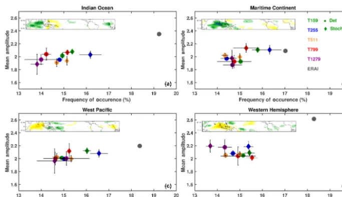
precipita-Figure 8.MJO frequency of occurrence vs. mean amplitude for the PDA experiments in the four different phases given the MJO amplitude to be>1. The four phases are classified as Indian Ocean(a), Maritime Continent(b), western Pacific (c)and western hemisphere(d), and their geographical location is shown by the boxes at the bottom of each panel with anomalous positive/negative precipitation patterns (green/yellow regions). Colours indicate the ensemble mean of the different resolutions as shown in the legend, where the circles are the deterministic runs and the diamonds the stochastic runs. ERA-Interim is reported in grey. Statistics are shown for the period 1980–2001. Error bars show the uncertainty range by providing the same statistic for periods half the length of the analysis.
tion followed by subsequent rainfall suppression (Khouider et al., 2011; Zhang et al., 2013; Kim et al., 2014; Raymond et al., 2015). It is a challenge for the current generation of global climate and weather models to represent the dynamics and thermodynamics of the MJO realistically (Slingo et al., 1996; Lin et al., 2006; Kim et al., 2009; Sperber et al., 2011; Klingaman et al., 2015).
Here we use the Wheeler and Hendon (2004) technique to identify the dominant modes of variability in zonal winds and outgoing longwave radiation (OLR) in these model runs. Combined Empirical Orthogonal Functions (CEOFs) of in-traseasonal OLR, U850 (zonal winds at 850 hPa) and U200 (zonal winds at 200 hPa) are computed for each of the runs. The first two leading modes (Realtime Multivariate MJOs: RMM1 and RMM2) correspond to MJO signatures in the tropical wind field and OLR. The amplitude Aof the MJO is defined as
A=p(RMM1)2+(RMM2)2 (3)
and the phase8of the MJO is defined as
8=tan−1
RMM2 RMM1
. (4)
MJO occurrence is defined when the MJO A is >1. Conventionally, eight phases of the MJO are defined (Gottschalck et al., 2010). We reduce the eight phases to four phases respectively corresponding to the MJO being active in the Indian Ocean, Maritime Continent, Western Pacific and Western Hemisphere. We note that the Wheeler Hen-don RMM index has been shown to be deficient in detecting
MJO events when large-scale circulation signals of the MJO are missing (Straub, 2013). Figure 8 shows the frequency of occurrence vs. the mean amplitude of the MJO in the four different regions around the tropics for all the different runs (colours) and for ECMWF ERA-Interim Reanalysis (grey; Dee et al., 2011) over the 1980–2001 period.
Overall the frequency of occurrence of the MJO in the dif-ferent regions in the tropics for the difdif-ferent model resolu-tions is underestimated with respect to that of ERA-Interim. The MJO amplitude in the model simulations is lower than reanalysis over the Indian Ocean and the Western Hemi-sphere.
More importantly, increasing horizontal resolution does not seem to improve the representation of the phenomenon significantly. This may be explained considering that the simulation of the MJO in GCMs is influenced primarily by the representation of mesoscale dynamics and of convection. The simulation of mesoscale dynamics can be helped by in-creasing the resolution, while improvements in convection are driven by changes in physical parameterisations of the model. Yet, the coupling between the mesoscale dynamics and the convection is key for convectively coupled waves in the tropics (Raymond et al., 2015). Therefore, increasing res-olution alone may not be sufficient to improve the simulation of the MJO.
therefore, a sampling error due to natural variability should be considered. Above all, the best results are obtained for the T255 with stochastic physics, suggesting that the tuning of the mean state of the model might play a relevant role for a better MJO simulation.
Additionally, the stochastic physics climate runs show an improvement in the representation of the MJO propagation over the Maritime Continent (not shown). The lack of prop-agation of the MJO over the Maritime Continent into the western Pacific region is a known problem in GCMs (Zhang et al., 2013). An improvement in the MJO propagation past the Maritime Continent due to SPPT has also been seen in the ECMWF seasonal forecasting system 4 (Weisheimer et al., 2014). Subramanian et al. (2017) also showed an improved MJO propagation and improved probabilistic prediction skill for the MJO in the ECMWF system 4 when SPPT is active as compared to runs without stochastic physics. Such improved propagation in stochastic runs indicates either that there is an impact of the stochastic physics on the mean state in the re-gion or that the variability in the rere-gion helps maintain the intraseasonal signal. The reasons for the change in MJO rep-resentation due to stochastic physics will be explored further in a more detailed future study by the authors.
5.4 Mid-latitude atmospheric blocking variability One of the most important challenges for the current gen-eration of climate models is the simulation of atmospheric blocking (Anstey et al., 2013; Masato et al., 2013; Dunn-Sigouin and Son, 2013; Davini and D’Andrea, 2016). Block-ing is a recurrent weather pattern typically occurrBlock-ing in the Northern Hemisphere at the exit of the Atlantic and Pacific jet stream, more frequently during the winter season but ob-served throughout the year (Rex, 1950; Tibaldi and Molteni, 1990). It is characterised by a high-pressure, long-lasting low-vorticity anomaly that “blocks” the mid-latitude west-erly flow, diverting synoptic disturbances poleward or equa-torward (Tyrlis and Hoskins, 2008; Davini et al., 2012). A blocking event can last several days or even weeks, and it may be associated with cold spells in winter and heat waves in summer (Sillmann et al., 2011; Dole et al., 2011).
Blocking here is diagnosed using the simple index intro-duced by D’Andrea et al. (1998), an extension of the better known Tibaldi and Molteni (1990) index. This 1-D block-ing index detects the reversal of the zonal flow measurblock-ing the geopotential height gradient at 500 hPa at 60◦N, providing a binary blocking time series for each longitude. Although there is some evidence (e.g. Berner et al., 2012; Dawson and Palmer, 2015) that stochastic physics may improve the blocking simulation, with the current diagnostic no statisti-cally significant difference emerges – even at low resolution – when comparing deterministic and stochastic simulations. Therefore, the two simulations are combined together to pro-vide an unique ensemble.
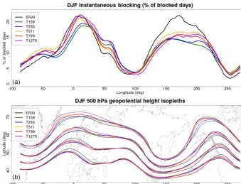
The upper panel of Fig. 9 shows the blocking frequency for the ERA-Interim Reanalysis (black) and the ensemble mean of the different horizontal resolutions (colours) of PDA ex-periments over the December–January–February (DJF) pe-riod. The common negative bias over the Atlantic and Pacific basins is clearly evident. Increasing the horizontal resolution leads to benefits over both the basins, with marked improve-ments especially for the Atlantic; here, T799 and T1279 runs show values comparable to the reanalysis. The largest im-provement is, however, seen upgrading from T255 to T511, where the bias – measured as the relative difference between the blocking frequency averaged between 10◦W and 30◦E – is reduced from the 18 to 3 %.
Those clear improvements in blocking frequency are in-terestingly reflected by a change in the mean state. A simple way to represent the flow variability is to highlight a few iso-pleths of geopotential height, as done in the lower panel of Fig. 9. Indeed, the higher-resolution models show a strength-ened pattern of the dominant Northern Hemisphere planetary waves, with marked ridges over the Rockies and Europe. Es-pecially, the former over the Rockies (Brayshaw et al., 2009) suggests an important role of orography resolution in the rep-resentation of the eddy-driven jet stream and, indirectly, of Euro-Atlantic blocking frequencies.
Indeed, the reduction of the bias following resolution in-crease for winter Atlantic blocking (and not for Pacific block-ing) seems to be a common feature of several GCMs (Davini and D’Andrea, 2016; Schiemann et al., 2016). Such im-provements have been associated with both better resolved transient eddy activity – which should sustain the blocking persistence (Shutts, 1983; Berckmans et al., 2013) – and with higher orography variance – which affects the mean state through planetary waves shaping (Jung et al., 2012; Berckmans et al., 2013). Conversely, Pacific blocking has been shown to be phenomenologically different (Pelly and Hoskins, 2003; Davini et al., 2012) and to be strongly af-fected by tropical dynamics (e.g. Renwick and Wallace, 1996); therefore, it is not surprising that the latter would be less affected by horizontal resolution changes.
A more detailed analysis of blocking and mid-latitude variability will be carried out by the authors in future studies.
6 Conclusions
forc-Figure 9. (a)Ensemble mean blocking frequencies following D’Andrea et al. (1998) for the different PDA experiments. Members of deter-ministic and stochastic experiments have been combined together for each resolution. ERA-Interim for the 1979–2008 period is shown as comparison in black.(b)December–January–February (DJF) climatological mean for geopotential height at 500 hPa for the ensemble mean of PDA experiments. Only 5200, 5300, 5400 and 5500 m isopleths are reported.
ing. These have been run at five different horizontal resolu-tions – spanning from 125 to 16 km – with several ensem-ble members. Furthermore, a smaller set of transient coupled simulations (PFC simulations, 1850–2100) at T255 ORCA1 (∼80 km for the atmosphere and about 1◦for the ocean) has been run.
Each deterministic experiment included in Climate SPHINX has a counterpart where the sub-grid unresolved scales have been parameterised with two different stochas-tic physics schemes (namely the SPPT and SKEB schemes). This makes Climate SPHINX the first climate dataset that in-cludes a large number of ensemble members with a stochas-tic parameterisation at different horizontal resolution; along with other high-resolution simulation campaigns such as UP-SCALE (Mizielinski et al., 2014) or ATHENA (Kinter III et al., 2013), this demonstrates the ability of the climate com-munity to exploit the more recent HPC machines.
Details on the tuning procedure (aimed at providing a cor-rect radiation budget in the standard configuration T255) have been presented. Moreover, a comprehensive description of the methodology adopted for the creation of the present-day and future scenario SST and SIC (starting from the HadISST 2.1.1 dataset) has been described. A novel method aimed at estimating SST, where SICs have disappeared in fu-ture climate simulations, has been introduced.
More importantly, Climate SPHINX post-processed out-puts are freely accessible to the climate community. This has been possible thanks to an EUDAT pilot project, which makes available a THREDDS server operational at CINECA from which data can be easily downloaded.
Preliminary results show the importance of both resolu-tion and stochastic perturbaresolu-tions on the representaresolu-tion of the climate variability, although different phenomena show dif-ferent sensitivities. Tropical rainfall variability seems to ben-efit from both increased horizontal resolution and stochas-tic parameterisation, whereas the Madden–Julian Oscillation shows improvements only when the stochastic perturbations are added. In general – in the tropics – applying stochastic schemes at low resolution leads to interesting improvements; on the other hand, increasing resolution beyond T511 does not seem to further improve the tropical variability.
members, suggesting that a single realisation may be not enough to capture the real sensitivity of this diagnostic to stochastic schemes. On the other hand, we found that in-creased horizontal resolution seems extremely important to decrease the blocking bias; in agreement with other recent works (Davini and D’Andrea, 2016; Schiemann et al., 2016) this is true especially over the Euro-Atlantic sector – where the T799 resolution (∼25 km) reduces it to negligible values – but not evident over the Pacific.
To summarise, the best improvements are observed on up-grading from T255 to T511, whereas minor improvements are observed using higher resolutions. However, while this resolution increase reduces the bias for the most of the phe-nomena here analysed, SPPT and SKEB schemes seem infective on some aspects (e.g. atmospheric blocking) but ef-fective as much as resolution – and even more – on others (e.g. tropical precipitation variability); in the case of the MJO variability, stochastic schemes applied to the T255 model bring improvements larger than the ones associated with any resolution refinement.
However, we must remark that these results can be asso-ciated with the absence of specific tuning for both determin-istic higher-resolution and stochastic configurations, which can affect the mean climate and consequently partially dete-riorate the climate variability. Indeed, such tuning does not involve only the surface and TOA radiative fluxes but also some of the physical parameterisations of the climate model. Some schemes, e.g. deep and shallow convection parameter-isations, may be satisfactory at coarse resolutions but may perform poorly at finer ones.
Given the similarities between the dynamical cores of cli-mate models, since they are all based on a controlled dis-cretisation of the same governing equations, we hope that the resolution sensitivity aspect of Climate SPHINX will be useful to the whole climate modelling community. On the other hand, several promising stochastic schemes exist, and the sensitivity of EC-Earth to SPPT and SKEB described here cannot be easily extrapolated to these alternative ap-proaches. Nevertheless, considering that Climate SPHINX is the first large experiment where stochastic schemes are used massively on the climate time range, we hope that this work paves the way for other climate-oriented simulations aimed at investigating the impact of different stochastic schemes on climate variability.
Furthermore, Climate SPHINX focuses attention on the controversial choice between increasing resolution or in-creasing the size of ensembles – whilst keeping the same computing time available (e.g. Buizza et al., 1998). Indeed, running 30 years of one member at T1279 on the SuperMUC Petascale System costs about 1.4 million core hours; with the same amount of time it would be possible to run 9–10 sim-ulations at T511. However, the benefits of the two pathways may be different, while a single member with 16 km reso-lution can provide local information at a topographic scale, which is useful, for instance, for hydrological models –
par-ticularly in areas with complex topography; in contrast many ensemble members at 40 km resolution can provide a cor-rect assessment of the natural variability, a key element for instance for mid-latitude climate (Deser et al., 2012; Kay et al., 2015). However, we must keep in mind that the com-putational constraints would become particularly relevant for coupled simulations, in which the computing time devoted to the oceanic model and – above all – to the spin-up of the coupled system will inflate considerably the number of core hours needed. Stochastic physics parameterisations, es-pecially at lower resolution, seem able to provide an interest-ing alternative to tackle such controversy, improvinterest-ing model performance without increasing the nominal resolution and the overall computational cost.
Data availability. Post-processed data have been transferred from LRZ to CINECA via GridFTP, where they have been permanently stored. More importantly, free data accessibility to the climate user community is granted through a dedicated THREDDS Web Server hosted by CINECA (https://sphinx.hpc.cineca.it/thredds/ sphinx.html), where it is possible to browse and directly down-load Climate SPHINX data. Details on the data accessibil-ity and on the Climate SPHINX project itself are available on the website of the project (http://www.to.isac.cnr.it/sphinx/). The set-up of this infrastructure for data sharing has been possible thanks to DATA SPHINX, an EUDAT data pilot project, which will allow long-term storage and sharing among a wide scientific user community of high-resolution climate model output data. DATA SPHINX aims to build a repository serving the climate change impact modelling community, providing selected variables at high temporal and spatial resolution, with a focus on climate extremes and the hydrological cycle in areas with complex orography.
Competing interests. The authors declare that they have no conflict of interest.
Seventh Framework Research Programme. The authors also acknowledge support by the PRIMAVERA project, funded by the European Commission under grant agreement no. 641727 of the Horizon 2020 Research Programme. Jost von Hardenberg acknowl-edges support from the European Union’s Horizon 2020 research and innovation programme under grant agreement no. 641816 (CRESCENDO) and thanks ECMWF for providing computing time in the framework of the special project SPITVONH.
Edited by: W. Hazeleger
Reviewed by: two anonymous referees
References
Anstey, J. A., Davini, P., Gray, L. J., Woollings, T. J., Butchart, N., Cagnazzo, C., Christiansen, B., Hardiman, S. C., Osprey, S. M., and Yang, S.: Multi-´model analysis of Northern Hemisphere winter blocking: Model biases and the role of resolution, J. Geo-phys. Res.-Atmos., 118, 3956–3971, 2013.
Arnold, H., Moroz, I., and Palmer, T.: Stochastic parametrizations and model uncertainty in the Lorenz’96 system, Philos. T. R. Soc. Lond, 371, 20110479, doi:10.1098/rsta.2011.0479, 2013. Balsamo, G., Viterbo, P., Beljaars, A., van den Hurk, B., Hirschi,
M., Betts, A. K., and Scipal, K.: A revised hydrology for the ECMWF model: Verification from field site to terrestrial water storage and impact in the Integrated Forecast System, J. Hydrom-eteorol., 10, 623–643, 2009.
Beljaars, A., Bechtold, P., Köhler, M., Morcrette, J.-J., Tomp-kins, A., Viterbo, P., and Wedi, N.: The numerics of physical parametrization, Proc. of ECMWF Seminar on Recent Develop-ments in Numerical Methods for Atmosphere and Ocean Mod-elling, ECMWF, Reading, UK, 2004.
Bengtsson, L., Steinheimer, M., Bechtold, P., and Geleyn, J.-F.: A stochastic parametrization for deep convection using cellular au-tomata, Q. J. Roy. Meteor. Soc., 139, 1533–1543, 2013. Berckmans, J., Woollings, T., Demory, M.-E., Vidale, P.-L., and
Roberts, M.: Atmospheric blocking in a high resolution climate model: influences of mean state, orography and eddy forcing, At-mos. Sci. Lett., 14, 34–40, 2013.
Berner, J., Shutts, G., Leutbecher, M., and Palmer, T.: A spectral stochastic kinetic energy backscatter scheme and its impact on flow-dependent predictability in the ECMWF ensemble predic-tion system, J. Atmos. Sci., 66, 603–626, 2009.
Berner, J., Jung, T., and Palmer, T.: Systematic model error: the im-pact of increased horizontal resolution versus improved stochas-tic and determinisstochas-tic parameterizations, J. Climate, 25, 4946– 4962, 2012.
Bouttier, F., Vié, B., Nuissier, O., and Raynaud, L.: Impact of stochastic physics in a convection-permitting ensemble, Mon. Weather Rev., 140, 3706–3721, 2012.
Brayshaw, D., Hoskins, B., and Blackburn, M.: The basic ingredi-ents of the North Atlantic storm track, Part I: land–sea contrast and orography, J. Atmos. Sci., 66, 2539–2558, 2009.
Buizza, R., Petroliagis, T., Palmer, T., Barkmeijer, J., Hamrud, M., Hollingsworth, A., Simmons, A., and Wedi, N.: Impact of model resolution and ensemble size on the performance of an ensem-ble prediction system, Q. J. Roy. Meteor. Soc., 124, 1935–1960, 1998.
Christensen, H. M., Moroz, I. M., and Palmer, T. N.: Simulating Weather Regimes: impact of stochastic and perturbed parame-ter schemes in a simple atmospheric model, Clim. Dynam., 44, 2195–2214, 2015.
Christensen, H. M., Berner, J., Coleman, D., and Palmer, T. N.: Stochastic parametrisation and the El Niño-Southern Oscillation, J. Climate, 30, 17–38, 2017a.
Christensen, H. M., Dawson, A., and Palmer, T.: Constrain-ing Stochastic Parametrisation Schemes usConstrain-ing High-resolution Model Simulations, in preparation, 2017b.
D’Andrea, F., Tibaldi, S., Blackburn, M., Boer, G., Deque, M., Dix, M. R., Dugas, B., Ferranti, L., Iwasaki, T., Kitoh, A., Pope, V., Randall, D., Roeckner, E., Straus, D., Stern, W., den Dool, H. V., and Williamson, D.: Northern Hemisphere atmospheric blocking as simulated by 15 atmospheric general circulation models in the period 1979–1988, Clim. Dynam., 14, 383–407, 1998.
Davini, P. and D’Andrea, F.: Northern Hemisphere atmo-spheric blocking representation in Global Climate Models: twenty years of improvements?, J. Climate, 29, 8823–8840, doi:10.1175/JCLI-D-16-0242.1, 2016.
Davini, P., Cagnazzo, C., Gualdi, S., and Navarra, A.: Bidimen-sional diagnostics, variability and trends of Northern Hemisphere blocking, J. Climate, 25, 6996–6509, 2012.
Davini, P., Filippi, L., and von Hardenberg, J.: Tuning EC-Earth from v3.01 to v3.1, Tech. Rep. 01/14, CNR-ISAC, UOS Torino, 2014.
Dawson, A. and Palmer, T.: Simulating weather regimes: impact of model resolution and stochastic parameterization, Clim. Dynam., 44, 2177–2193, 2015.
Dawson, A., Palmer, T., and Corti, S.: Simulating regime structures in weather and climate prediction models, Geophys. Res. Lett., 39, L21805, doi:10.1029/2012GL053284, 2012.
Dee, D. P., Uppala, S. M., Simmons, A. J., Berrisford, P., Poli, P., Kobayashi, S., Andrae, U., Balmaseda, M. A., Balsamo, G., Bauer, P., Bechtold, P., Beljaars, A. C. M., van de Berg, I., Biblot, J., Bormann, N., Delsol, C., Dragani, R., Fuentes, M., Greer, A. J., Haimberger, L., Healy, S. B., Hersbach, H., Holm, E. V., Isak-sen, L., Kallberg, P., Kohler, M., Matricardi, M., McNally, A. P., Mong-Sanz, B. M., Morcette, J.-J., Park, B.-K., Peubey, C., de Rosnay, P., Tavolato, C., Thepaut, J. N., and Vitart, F.: The ERA-Interim reanalysis: Configuration and performance of the data assimilation system, Q. J. Roy. Meteorol. Soc., 137, 553–597, 2011.
Delworth, T., Rosati, A., Anderson, W., Adcroft, A., Balaji, V., Ben-son, R., Dixon, K., Griffies, S., Lee, H., Pacanowski, R., Vecchi, G., Wittenberg, A., Zeng, F., and Zhang, R.: Simulated climate and climate change in the GFDL CM2. 5 high-resolution coupled climate model, J. Climate, 25, 2755–2781, 2012.
Demory, M.-E., Vidale, P. L., Roberts, M. J., Berrisford, P., Stra-chan, J., Schiemann, R., and Mizielinski, M. S.: The role of hori-zontal resolution in simulating drivers of the global hydrological cycle, Clim. Dynam., 42, 2201–2225, 2014.
Deng, Q., Khouider, B., and Majda, A. J.: The MJO in a coarse-resolution GCM with a stochastic multicloud parameterization, J. Atmos. Sci., 72, 55–74, 2015.