University of New Orleans University of New Orleans
ScholarWorks@UNO
ScholarWorks@UNO
University of New Orleans Theses and
Dissertations Dissertations and Theses
12-15-2006
Development of an Image Noise Estimation Method and a
Development of an Image Noise Estimation Method and a
Sub-Imaging Based Wiener Method
Imaging Based Wiener Method
Eric F. Smith
University of New Orleans
Follow this and additional works at: https://scholarworks.uno.edu/td
Recommended Citation Recommended Citation
Smith, Eric F., "Development of an Image Noise Estimation Method and a Sub-Imaging Based Wiener Method" (2006). University of New Orleans Theses and Dissertations. 1052.
Development of an
Image Noise Estimation Method
and a
Sub-Imaging Based Wiener Method
A Dissertation
Submitted to the Graduate Faculty of the University of New Orleans in partial fulfillment of the requirements for the degree of
Doctor of Philosophy in
Engineering and Applied Science
by
Eric F. Smith
A.S., Delgado Community College, 1996 B.S., University of New Orleans, 1988 M.S., University of New Orleans, 2002
ACKNOWLEDGMENT
TABLE OF CONTENTS
LIST OF FIGURES ...v
LIST OF TABLES... vii
LIST OF ABBREVIATIONS ... vii
ABSTRACT ... x
1 INTRODUCTION ...1
1.1Preliminaries ...3
1.2Image Domain Direct Method ...10
1.3Fourier Method ...11
1.4Wiener Method ...12
1.5Van Cittert Method ...14
1.6Richardson Lucy Method ...16
1.7CLEAN Method ...18
1.8Comparison of Methods...20
2 NOISE SIGMA ESTIMATION METHOD ...33
2.1Wavelet Noise Reduction Method ...34
2.2Morrison Noise Reduction Method ...40
2.3Comparison of MNRM and WNRM ...42
2.4Noise Sigma Estimation Method ...46
3 SUB-IMAGING METHOD...54
3.1Sub-Imaging ...55
3.2Sub-Imaging Wiener Method ...59
3.4Comparison of SIWM and MatLab Wiener2 ...68
4 SUMMERY AND DISCUSSION ...71
BIBLIOGRAPHY ...74
COMPUTER CODE ...76
LIST OF FIGURES
Figure 1.1. Image Contamination Model ...1
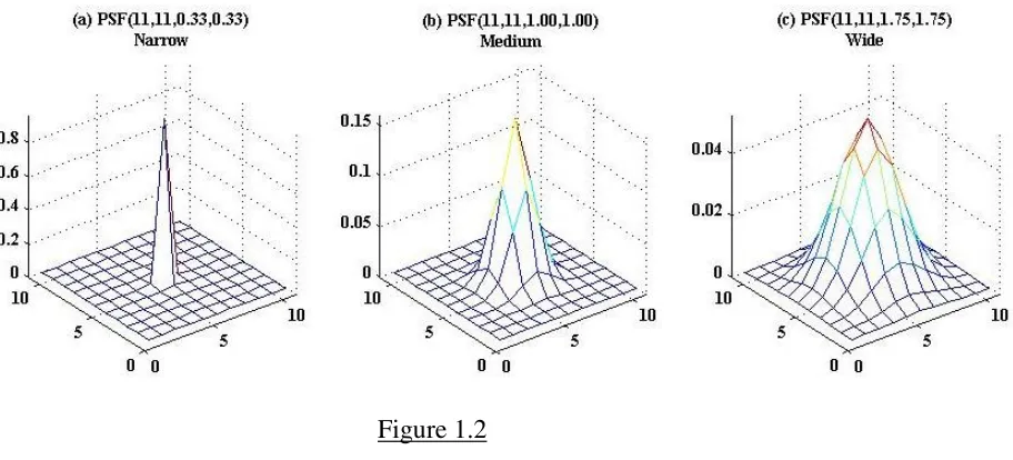
Figure 1.2. Narrow & Wide PSF ...3
Figure 1.3. B&W and Color Pixel Sample ...4
Figure 1.4. Example of Image Contamination ...7
Figure 1.5. Dr. Norbert Wiener ...12
Figure 1.6. Flow Chart of Wiener Method ...13
Figure 1.7. Flow Chart of VCM ...14
Figure 1.8. Flow Chart of RLM ...16
Figure 1.9. Flow Chart of CLEAN Method ...18
Figure 1.10. Images used in this Dissertation ...20
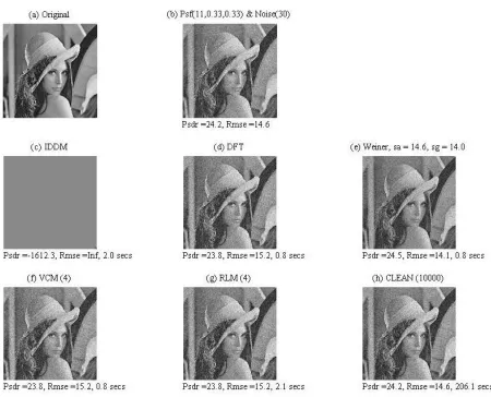
Figure 1.11. 6 Restoration Methods: Image 2 with PSF(11,0.33,0.33) & Noise(30) ...22
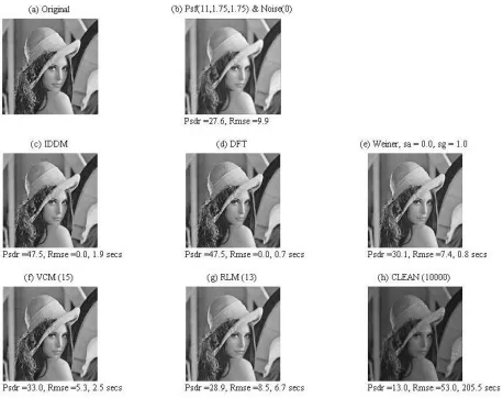
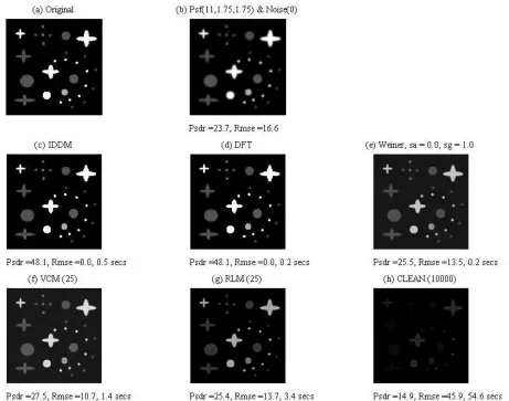
Figure 1.12. 6 Restoration Methods: Image 2 with PSF(11,1.75,1.75) & Noise(0) ...23
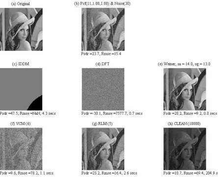
Figure 1.13. 6 Restoration Methods: Image 2 with PSF(11,1.,1.) & Noise(30) ...24
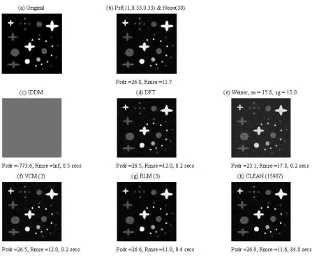
Figure 1.14. 6 Restoration Methods: Image 5 with PSF(11,0.33,0.33) & Noise(30) ...25
Figure 1.15. 6 Restoration Methods: Image 5 with PSF(11,1.75,1.75) & Noise(0) ...26
Figure 1.16. 6 Restoration Methods: Image 5 with PSF(11,1.,1.) & Noise(30) ...27
Figure 1.17. 6 Restoration Methods: Image 10 with PSF(11,1.,1.) & Noise(30) ...28
Figure 1.18. 6 Restoration Methods: Image 1 with PSF(11,1.,1.) & Noise(30) ...29
Figure 2.1. Flow Chart of Daubechies Coefficients ...36
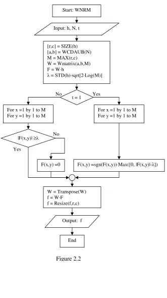
Figure 2.2. Flow Chart of WNRM...37
Figure 2.4. Flow Chart of Morrison Noise Reduction Method (MNRM) ...41
Figure 2.5. MNRM and WNRM, narrow width PSF: Image 3...42
Figure 2.6. MNRM and WNRM, medium width PSF: Image 8 ...43
Figure 2.7. MNRM and WNRM, wide width PSF: Image 10 ...44
Figure 2.8. Flow Chart of Sigma Estimation Method (SIGEST) ...46
Figure 2.9. Graph of Sigma actual vs Sigma estimated ...48
Figure 2.10. MNRM with narrow PSF: Images 1 and 8 ...53
Figure 3.1. Flow Chart of CALC_ASI ...55
Figure 3.2. Example of SIM applied to Image 2 (all sub-images)...56
Figure 3.3. Example of SIM applied to Image 2 (one sub-images) ...57
Figure 3.4. Example of SIM applied to Image 1 ...58
Figure 3.5. Flow Chart of SIWM ...59
Figure 3.6. SIM Applied to Image 9 ...61
Figure 3.7. SIM Applied to Image 14 ...62
Figure 3.8. SIM Applied to Image 1 ...63
Figure 3.9. SIWM vs Wiener 2: Image 13 ...68
Figure 3.10. SIWM vs Wiener 2: Image 9 ...69
Figure 3.11. SIWM vs Wiener 2: Image 9 ...69
LIST OF TABLES
Table 1.1. Simulation results for PSF(11,1.0,1.0) and Noise(30)...30
Table 2.1. Noise Estimation Results for WNRM ...39
Table 2.2. Noise Estimation Results for narrow width PSF ...49
Table 2.3. Noise Estimation Results for medium width PSF ...50
Table 2.4. Noise Estimation Results for wide width PSF ...51
Table 3.1. SIWM Results for Images: 1, 2, 4, 7, 9 to 14, narrow PSF ...64
Table 3.2. SIWM Results for Images: 1, 2, 4, 7, 9 to 14, meduim PSF ...65
LIST OF ABBREVIATIONS
h Recorded image data
h2 Image data processed by two iterations of the Morrison Noise Reduction Method
hN Image noise data calculated by, hN = h – h2 PSF Point spread function
b Blurring function (PSF), also impulse response
n Noise data
f Actual image data (uncontaminated), in optics called object data Psdr Peak signal to distortion ratio
Rmse Root mean square error mse Mean square error ** Convolution operator DFT Discrete Fourier transform
IDFT Inverse discrete Fourier transform
B
b⊃ Fourier transform of b into B
b
B⊂ Inverse Fourier transform from B to b
σf Standard deviation of image data f
FTM Fourier Transform Method VCM Van Cittert Method
RLM Richardson Lucy Method
MNRM Morrison Noise Reduction Method SIGEST Sigma Estimation Method
SIM Sub-Imaging Method
SIWM Sub-Image Wiener Method
ABSTRACT
This research consists of three parts. The first part is an investigation of several popular image restoration techniques. The techniques are used to restore 2-D image data, f(x,y), that has been blurred by a known point spread function (PSF), b(x,y) and corrupted by an unknown amount of noise, n(x,y). Several sample images are restored using all of the techniques. Of the methods investigated the one which produces the best restoration results was determined to be the Wiener deconvolution method. The determination of the best method is based on the quality of the restored image and the required restoration time.
The second part of this research involves the development of a noise standard deviation (σn) estimation method. The method determines an estimate, σe, of σn based on the Morrison Noise Reduction Method (MNRM) and is therefore an iterative method. The results of the noise, σn, estimating method (SIGEST) developed are rather good. The error between σn and σe when average across several images all contaminated with a medium width or greater PSF and various amounts of noise, is less than 10 percent. Knowledge of σn is important for the application of Wiener deconvolution. All noise in this research is assumed to be uncorrelated noise.
The third part of this research involves the development of the Sub-Imaging Method, SIM. In the third part of this research, the h2 and the hN of image data h is defined as follows:
which is closest to the average of all the σe‘s. The part with a σe closest to the average is defined to be the average sub-image (asi). The following assertions concerning SIM are investigated:
1. The asi of an image can be used in the place of the whole image to determine σe of σn and used to restore the whole image. Therefore, the noise in a piece of an image can represent the noise in the whole image (provided it is the asi of the image’s hN). 2. SIM can be combined with the Wiener image restoration method to restore
contaminated image data without the σn of the data initially being known.
CHAPTER 1
INTRODUCTION
“One picture is worth more than ten thousand words”, is a familiar proverb that refers to the
idea that complex stories can be told with just a single still image. A single image may be more informative and or influential than a substantial amount of written information. An image may be defined as a two-dimensional function, f(x,y), where x and y are spatial coordinates, and the amplitude of f at any location (x,y) is called the intensity or gray level of the image at that point, [8]. Joseph Nicéphore Niépce using a sliding wooden box camera made by Charles and Vincent Chevalier in Paris made the first permanent image (photograph) in 1826 or 1827. In many applications (e.g., satellite imaging, medical imaging, astronomical imaging, poor-quality family portraits) the imaging system introduces a slight distortion. Often images are slightly blurred and image restoration aims at deblurring the image.
Digital image processing is the manipulation of images by computer. One of the first applications of digital images was in the newspaper industry when pictures were first sent by submarine cable between London and New York in the 1920s. Digital image techniques in image restoration and enhancement had their first fruitful application at the Jet Propulsion
properties of the cameras before they were launched and then used computer processing to remove, as well as possible, the degradations from the received moon images, [2].
From the 1960s until the present, the field of image processing has grown significantly. In addition to applications in medicine and the space program, digital image processing techniques now are used in a broad range of applications. Computer procedures are used to enhance the contrast or code the intensity levels into color for easier interpretation of X-rays and other images used in industry, medicine, and the biological sciences. Geographers use the same or similar techniques to study pollution patterns from aerial and satellite imagery. Image
1.1
Preliminaries
Deconvolution is a process of recovering information which has been altered (contaminated) from its true original form. The contamination for many images has two basic forms: blurring, which is described by the convolution, and noise addition. Thus contamination can be modeled as follows:
Figure 1.1
). , ( ) , ( * * ) , ( ) , ( ], 1 . 1
[ h x y =b x y f x y +n x y
h = Recorded image data.
b = Blurring function or point spread function (PSF), also called the impulse response. n = Noise
f = Actual input data (uncontaminated), referred to in optics as the object data. The symbol ** denotes convolution between the PSF and the actual data.
Convolution describes the action of an observing instrument; it is generally a smoothing process. Mathematically, 2D convolution is defined (continuous and discrete variables respectively) as follows,
b(x,y)
n(x,y)
A numerical example of 2D convolution is shown in equation 1.4. . 24 22 15 9 40 45 39 18 18 30 31 11 2 7 7 2 6 1 3 7 4 5 1 3 2 4 3 2 1 ], 4 . 1
[ b f =h
= ∗ ∗ = ∗ ∗
Noise is whatever distorts, deforms, prevents, interferes or changes the information being observed and or recorded other than that caused by a devices lens. In this paper all noise is considered to be normally distributed (gaussian) with a mean of zero. In my research I added noise to the various input image data by generating a random matrix using the Matlab function randn. The function randn, generates random normally distributed values with a standard deviation of 1, the values are stored in the noise matrix, inoise. The following equation is used to create the 2D noise matrix n(x,y) used in equation 1.1:
. 100 )] ( ) ( [ ) , ( ) , ( ], 5 . 1
[ n x y =inoise x y ⋅ Max f −Min f ⋅ns
In equation 1.5, the value of ns is arbitrarily set from 0 to 100, so that the noise is set to have a σn which is ns% of the range of values of f, the original image data. To ensure the non-negativity of h calculated in equation 1.1 and that it not exceed the maximum pixel value, if h is less than zero then it’s value is set equal to zero and if it is greater than 255 then it is set equal to 255.
. 2 2 exp 2 1 ) , , , ( ], 6 . 1 [ 2 2 2 2 2 2 ⋅ − + ⋅ − ⋅ ⋅ ⋅ ⋅ = y x y x y x y x y x N N PSF
σ
σ
σ
σ
π
σ
σ
In equation 1.6, x runs from -Nx/2 to Nx/2 and y from -Ny/2 to Ny/2. The size of the matrix generated is Nx by Ny. The variables σx and σy are the standard deviation in the x and y direction respectively. For example, a 11 by 11 narrow PSF is given by, b = PSF(11,11,0.33,0.33), and is shown in figure 1.2a, a medium width PSF is given by b = PSF(11,11,1.0,1.0) shown in figure 1.2b and a 11 by 11 wide PSF is given by, b = PSF(11,11,1.75,1.75), shown is shown in figure 1.2c. All of the PSF’s used in this paper are square in size, so hencforth all PSF’s will be indicated by PSF(Nxy, σx, σy), with Nxy = Nx = Ny. Also from this point forward the amount of noise added to an image will be indicated by Noise(ns), the function which creates the noise matrix n(x,y) used in equation 1.1.
deconvolution, which will not be considered in this research, [14]. The MatLab code (m files) are shown in the Code section of this dissertation. Knowledge of the PSF b is possible because the blurring caused by a measuring instrument can be determined. The PSF is mostly a function of an instrument’s lens for many optical systems.
The 2D image data contained in h and f specifies the light intensity measured from 0 through 255 for this research. An example of black and white image data stored in f1 is shown in
equation 1.7. Each pixel in an image has an intensity value, [6]. The y and x index of the intensity corresponds to its position, e.g., f(2,4) = 220 means at position 2 units vertical and 4 units horizontal the light intensity is 220. The image generated by the f1 data is shown in figure 1.3a. An example of color image data f2 is shown in equation 1.8, each pixel is made of three separate intensities: red (f2(:,:,1)), green (f2(:,:,2)) and blue (f2(:,:,3)), [19]. The image generated by f2 is shown in figure 1.3b.
Figure 1.3
Two criteria which are used to indicate how well the image g has been restored from the measured image data h are psdr and rmse. The peak signal to distortion (blur and noise) ratio (psdr), the root mean square error (rmse) and the mean square error (mse) are calculated as follows: . ], 9 . 1
[ Nrc = Nr⋅Nc
. || ) , ( ) , ( || 1 ], 10 . 1 [ 2
∑∑
− = r c N i N j rc j i g j i f N mse . ], 11 . 1[ rmse= mse
). ) ( ( 20 ], 12 . 1
[ psdr = ⋅Log Max g rmse
In equation 1.9, Nr and Nc are the number of pixels in each row and column of the image respectively, and Nrc is the total number of pixels in the image. Note that in equation 1.12 the psdr is given in dB. The smaller the value of rmse the closer g is to f by this measure. The greater the value of psdr the less noise and blurring are in the restored image g although the value of maximum g also enters the result.
The average pixel intensity of f isp, the variance of image data f is σf2, and the standard
deviation of f is σf shown in equations 1.13, 1.14 and 1.15 respectively. The standard deviation of f is the statistical measure of spread or variability of the pixel intensities in f.
. ) , ( 1 ], 13 . 1 [ 1 1
∑∑
= = = r c N r N c rc c r f N p . ] ) , ( [ ) 1 ( ) 1 ( 1 ], 14 . 1 [ 1 1 2 2∑∑
= = − − ⋅ − = r c N r N c c rf f r c p
N N
σ
. ], 15 . 1The discrete Fourier transform (DFT) of f and the inverse discrete Fourier transform (IDFT) of F are defined in equations 1.16 and 1.17 respectively.
. )] / / ( 2 exp[ ) , ( ) , ( ) ( ], 16 . 1 [ 1 0 1 0
∑ ∑
− = − = − ⋅ − ⋅ = = r c N j N k cr yk N
N j x i y x f k j F f DFT
π
. )] / / ( 2 exp[ ) , ( 1 ) , ( ) ( ], 17 . 1 [ 1 0 1 0∑ ∑
− = − = − ⋅ ⋅ = = r c N j N k c r rc N k y N j x i k j F N y x f F IDFTπ
1.2
Image Domain Direct Method
The Image Domain Direct method, IDDM, is a direct method that solves equation 1.1, with zero noise, algebraically for f [13]. The original image data f, is solved for by executing equation 1.18 for all x from 1 to Nx and y from 1 to Ny.
. ) 1 , 1 ( )) 1 ( ), 1 (( ) , ( ) , ( ) , ( ], 18 . 1
[ 1 1
b c y r x f c r b y x h y x f J r K c
∑∑
= = + − + − − = Where, )). 1 ( ), ( ( ], 19 . 1[ J =Min Rows b x−
)). 1 ( ), ( ( ], 20 . 1
[ K =Min Cols b y−
Advantages of the method:
1. Restores f very well, with b known and zero noise. Disadvantages of the method:
1. Is extremely sensitive to noise.
2. Is computationally expensive and slow.
3. If b(1,1) equals zero, PSF must be shifted to solve for f.
1.3
Fourier Transform Method
The Fourier transform method is a direct method that solves equation 1.1, with zero noise, for f by first calculating the Fourier transform of h⊃Hand of b⊃B, [13]. By the convolution theorem,
. ],
21 . 1
[ b∗∗f =h⊃ H =B⋅F
with B · F, in equation 1.21, the point wise product of matrices B and F. Thus,
, ],
22 . 1
[ F =H B and
). ( ],
23 . 1
[ f =IDFT F
Advantages of the method:
1. Restores f very well, with zero noise.
2. Is computationally fast (especially compared to the direct method). Disadvantages of the method:
1. Is sensitive to noise.
This method restores the image data very well, provided the image contains zero noise and has a known PSF. The MatLab code for this method is in file “ftm.m”. The code is shown in the code section of this dissertation and several images restored by this method are shown in the
1.4
Wiener Method
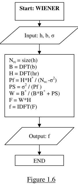
The Wiener method is an optimum linear noise and deconvolution filter based in the Fourier domain. It was invented by mathematician Norbert Wiener, [3]. Dr. Wiener first published the Wiener filter method in 1949. The method is a direct method that solves for f by using the power spectra of the noise, Pn, and image data, Pf, by the following equations, which also show the approximations used in this dissertation, [15] [5] [17]:
. ], 24 . 1 [ * rc n N N N
P = ⋅
. ], 25 . 1 [ * rc f N F F
P = ⋅
, ˆ ], 26 . 1
[ Pn ≈
σ
n2 for white noise.. ˆ ], 27 . 1 [ 2 * n rc f N H H
P ≈ ⋅ −
σ
. ˆ ˆ | | | | ], 28 . 1 [ 2 * 2 * f n f
n B P P
B P P B B G + ≈ + =
Dr. Norbert Wiener 1894-1964 Figure 1.5 . ], 29 . 1
[ F =G⋅H
). ( ], 30 . 1
[ f =IDFT F
Advantages of the method:
1. Can restore f with noise present. Disadvantages of the method:
2. Requires knowledge of Pn or an approximation such as by equation 1.26, which then requires knowledge of σn or an estimate of it.
This method restores the image data with a known PSF and noise present. A flowchart of the method is shown in figure 1.5 and the MatLab code for this method is in file “dwiener.m”. The code is shown in the code section of this dissertation and several images restored by this method are shown in the Comparison of Methods section. The Wiener method is known to be one of the best linear filters if Pf and the contaminating noise are known. It is derived to be the optimum filter in the least squares sense. Of course in reality neither the Pn nor Pf are known, but for white noise they can be approximated very well by equations 1.26 and 1.27.
Start: WIENER
Input: h, b, σ
Nrc = size(h)
B = DFT(b) H = DFT(hr) Pf = H*H* / (Nrc -σ
2
) PS = σ2 / (Pf ) W = B* / (B*B* + PS) F = W*H
f = IDFT(F)
1.5
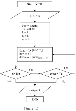
Van Cittert Method
The Van Cittert method is an iterative deconvolution method, [13]. It approximates f in equation 1.1, by setting an initial value f0 = f then iterating equation 1.31 an arbitrary maximum set
number of times (Nitr) or until the change in rmse is less than some set tolerance (Tol), [10].
]. [
], 31 . 1
[ fk+1 = fk + h−b∗∗fk
A flowchart of the method is shown in figure 1.7.
Start: VCM
h, b, Nitr
f(k+1) = fk+ [h-b**fk]
m = m +1
drmse = Rmse(f(k+1) , fk)
Output: f
END
Figure 1.7
No
Yes
m < Nitr
Nrc = size(h) Tol = 0.30 k = 1 fk = h
m = 1
No Yes
Advantages of the method:
1. Can restore f with noise present. Disadvantages of the method:
1. Number of iterations is by trial or estimate and or the value of the stopping tolerance is arbitrary.
1.6
Richardson Lucy Method
The Richardson Lucy method is an iterative deconvolution method, [13]. This method was developed from maximum likelihood theory and is modeled with Poisson statistics. It approximates f, with noise, by setting an initial value of f then iterating one of the following equations Nitr times, or until the change in rmse is less than some set tolerance (Tol):
}] ) ( { ) [( * ], 32 . 1
[ fk+1 = fk −b ∗∗ h b∗∗fk , Poisson Noise Model.
] ) ( [ * ], 33 . 1 [ 1 b f b h b f f k k k ∗ ∗ ∗ ∗ ∗ ∗ =
+ , Gaussian Noise Model.
A flowchart of the method, for gaussian noise, is shown in figure 1.8.
Start: RLM
h, b, Nitr
Figure 1.8
Nrc = size(h) Tol = 0.10 k = 1 fk = h
m = 1
f(k+1) = fk* [(b**h) / (b**fk**b)]
m = m +1
drmse = Rmse(f(k+1) , fk)
Output: f
END No
Yes m < Nitr
No drmse < Tol
Advantages of the method:
1. Can restore f with noise present. Disadvantages of the method:
1. Number of iterations is by trial or estimate and or the value of the stopping tolerance is arbitrary.
1.7
CLEAN Method
The CLEAN method is an iterative deconvolution method. CLEAN was developed by J. D. Hogbom in 1974, [21]. The method is nonlinear and deconvolves b, referred to as the “dirty beam”, from h, referred to as the “dirty image”. The algorithm involves the creation of a residual image R, and a density image, D, [22] [23]. The CLEAN algorithm is described by the flowchart in figure 1.9.
Start: CLEAN
h, b, Nitr, g
bc = zeros(size(b))
bc(center) = center pixel in b
D = 0 R = h M = 0
Locate max pixel intensity in R at (j,k), Pmax = R(j,k)
R = R – g·Pmax·b D(j,k) = D(j,k) + g·Pmax
f = D ** bc + R
Output: f
END
Figure 1.9
No Yes Pmax < TOL
The method assumes that the image (sky) brightness is essentially an ensemble of point sources (the sky is dark, but full of stars).
Advantages of the method:
1. Can restore f with noise present. Disadvantages of the method:
1. Requires a large number of iterations. 2. Number of iterations is by trial or estimate.
1.8
Comparison of Methods
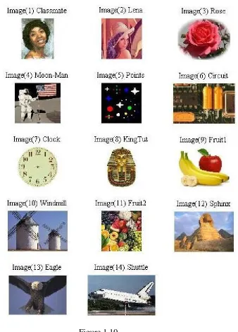
In this dissertation the images shown in figure 1.10 shall be used to evaluate the various image restoration methods and techniques.
The main objective of this section is to determine the best image restoration method of the six described in sections 1.1 through 1.6. The method selected must be able to restore an image that has been contaminated with blur and noise. The test comparison of the six methods is done using several of the images shown in figure 1.10. The images are contaminated in three different ways:
1. Blurred by a narrow width PSF(11,0.33,0.33) and Noise(30) 2. Blurred by a medium width PSF(11,1.75,1.75) and Noise(0) 3. Blurred by a wide width PSF(11,1.00,1.00) and with Noise(30)
The first contamination (simulation) represents contamination mostly due to noise. The second simulation represents contamination due to blurring with no noise. The third simulation
represents a moderate amount of contamination due to blurring and noise. The third simulation is done using images 2, 5, 10 and 1, and the first and second is done using images 2 and 5. The results of the simulation are shown in figures 11 through 17 and a summary of the third
Summary: Comparison Restoration Methods Results PSF(11,1.0,1.0) Noise(30)
Image Method Psdr Rmse Time Iterations Restored Best
(No.) sec Method
Lena Image data 23.7 15.4
(2) IDDM -Inf Inf 4.3 1 No DFT -30.1 7577.7 0.7 1 No
Weiner 28.2 9.2 0.8 1 Yes Yes
VCM 9.6 78.2 1.1 6 No RLM 23.2 16.4 2.6 5 Yes CLEAN 10.7 69.4 204.9 10000 No
Points Image data 23.6 16.8
(5) IDDM -Inf Inf 0.5 1 No DFT -26.7 5506.4 0.2 1 No
Weiner 24.3 15.6 0.2 1 Yes Yes
VCM 13.9 51.5 0.3 5 No RLM 23.8 16.5 0.7 5 Yes CLEAN 16.4 38.5 54.4 10000 No
Windmill Image data 22.1 19.8
(10) IDDM -Inf Inf 1.3 1 No DFT -30.1 8063.4 0.5 1 No
Weiner 24.7 14.7 0.6 1 Yes Yes
VCM 10.7 73.1 0.7 5 No RLM 22 20 1.5 4 Yes CLEAN 11 71.2 143.1 10000 No
Classmate Image data 21.8 20.8
(1) IDDM -Inf Inf 0.9 1 No DFT -30.1 8169.4 0.6 1 No
Weiner 23.8 16.4 0.4 1 Yes Yes
VCM 7.7 104.9 0.8 8 No RLM 21.5 21.5 1.3 5 Yes CLEAN 11.8 65.8 95.9 10000 No
The data in figures 1.11 through 1.18 indicate that the best direct method is the Wiener method. The Wiener method restored all of the test images, (although some better than others) for every type of PSF and amount of noise tested. If there is no noise contamination then the best method for giving the consistently lowest rmse is the IDDM, however the data show that it is one the slowest methods and real world data will almost always contain noise. The IDDM on average required 3 times more time than the next best non-noise handling method, the DFT method. If keeping the restoration time to a minimum is important then the DFT is a better method than the IDDM. The data show that the DFT can handle some noise unlike the IDDM, which did not restore any of the images with noise. However the DFT failed to restore images with moderate noise and a medium width PSF, as shown by figures 1.13, 1.16, 1.17 and 1.18. The data in table 1.1 shows that for the worst simulation case (moderate amounts of blur and noise) the best method based on highest PSDR and smallest RMSE is the Wiener and the second best is RLM.
type images, which is what it was originally designed for (recorded by an imaging system with a narrow PSF).
The data in figures 1.11 through 1.18 show the RLM and VCM to be better image restoration methods than the CLEAN method. In addition, the figures show that the RLM tends to converge to a solution in fewer iterations than the VCM and for the same number of iterations the VCM is the faster of the two. However the RLM produced better results for wide PSF’s than the VCM and has better noise handling abilities.
To summarize, the data in figures 1.11 through 1.18 and table 1.1 indicate that the best image restoration method in the presence of noise and blur, of the six investigated, is the Wiener
CHAPTER 2
NOISE SIGMA ESTIMATION METHOD
2.1
Wavelet Noise Reduction Method
Wavelets are mathematical functions that cut up data into different frequency components, and then study each component with a resolution matched to its scale. They have advantages over traditional Fourier methods in analyzing physical situations where the signal contains discontinuities and sharp spikes. Wavelets were developed independently in the fields of mathematics, quantum physics, electrical engineering, and seismic geophysics. Interchanges between these fields during the last twenty years have led to many new wavelet applications such as image compression, turbulence, human vision, radar, and earthquake prediction. In this
research, wavelets are used for de-noising 2-d image data.
The de-noising procedure of a noisy image can be divided into three stages, [25] [24]: 1) The wavelet transform of an image.
2) Thresholding of wavelet coefficients. 3) The inverse wavelet transform.
In the above stages, the vital key is stage (2), how to threshold the wavelet coefficients. For stage 1, the coefficients of the chosen wavelet must be calculated. I have chosen to use Daubechies wavelets, [4]. The coefficients, ak, are solved for from the following three conditions
2 ], 1 . 2 [ 1 =
∑
= N k k a 0 ) 1 ( ], 2 . 2 [ 1 1 1 = −∑
= − − N k m k k k a ) 1 , 0 ( 2 ], 3 . 2 [ 1 − =∑
= m a a N k u k δ2 1 2 1 2 1 2 1 0 0 0 0 0 0 0 0 ], 4 . 2 [ b b a a b b a a W = ) 1 ( 1 ) 1 ( ], 5 . 2
[ = − − N−k+
k k a b h W F = ], 6 . 2 [
For stage (2), thresholding is applied to F, that is the values in F belowλ are set equal to zero, this is called hard thresholding and is shown in equation 2.8. Soft thresholding is shown in equation 2.9 where the sgn(Fxy) is the sign of Fxy, [9] [7].
) log( 2 ) ( ], 7 . 2
[
λ
=STD h ⋅ M0 | | ], 8 . 2
[ if Fx,y ≥λ thenFx,y =Fx,y elseFx,y =
)]) | (| , 0 ([ ) sgn( ], 9 . 2
[ Fx,y = Fx,y ⋅Min Fx,y −λ
STD = Standard deviation, and M = height and width of W, (W is a square matrix). Next the de-noised image, f, is calculated using the inverse wavelet transform matrix which is equal to the transpose of the wavelet transform matrix.
F W f ' ], 10 . 2 [ =
Start: WCDAUB
Input: N
a = a / sqrt(2) k = 0
Output: a, b
End
Figure 2.1
N = 4 No a = [0.6830127,1.1830127,0.3169873,-0.1830127]
Yes
N = 6
No a = [0.47046721,1.14111692,0.650365,
-0.19093442,-0.12083221,0.0498175]
Yes
N = 8
No a =[0.3258034,1.0109457,0.892201,-0.0396750,
-0.2645071,0.0436163,0.046504,-0.0149869]
Yes
N = 16 No a = [0.0769556,0.4424672,0.9554861,0.8278165,
-0.0223857,-0.401658,6.68192e-4,0.1820766, -0.0245639,-0.062350,0.0197721,0.0123688, -6.8877e-3, -5.540e-4, 9.5522e-4,-1.66137e-4]
Yes
a = [1, 1]
k < N b(k) = (-1)^(k-1)·a(N-k+1)
k = k +1
Start: WNRM
Input: h, N, t
[r,c] = SIZE(h) [a,b] = WCDAUB(N) M = MAX(r,c) W = Wmatrix(a,b,M) F = W·h
λ = STD(h)·sqrt[2·Log(M)]
W = Transpose(W) f = W·F
f = Resize(f,r,c)
Output: f
End
Figure 2.2
t = 1
For x =1 by 1 to M For y =1 by 1 to M
|F(x,y)| ≥λ
F(x,y) =0 F(x,y) =sgn(F(x,y))·Max([0, |F(x,y)|-λ]) No Yes
Yes
No
Results of the WNRM applied to image data contaminated by a medium width PSF and Noise(30).
(a) Lena PSF(11,1,1) NS(30)
Method NI/WL PSDR RMSE Time
Actual 23.729 15.429
WNRM Soft-T D4 22.795 17.180 1.06 WNRM Soft-T D8 22.864 17.044 1.05 WNRM Soft-T D16 22.809 17.151 1.02 WNRM Hard-T D4 24.228 14.567 0.31 WNRM Hard-T D8 24.255 14.521 0.31 WNRM Hard-T D16 24.235 14.554 0.33
(b) Rose PSF(11,1,1) NS(30)
Method NI/WL PSDR RMSE Time
Actual 23.289 17.462
WNRM Soft-T D4 21.384 21.744 1.84 WNRM Soft-T D8 21.404 21.693 1.81 WNRM Soft-T D16 21.356 21.814 1.89 WNRM Hard-T D4 23.910 16.257 1.19 WNRM Hard-T D8 23.933 16.214 1.17 WNRM Hard-T D16 23.863 16.345 1.19
(c) Circuit PSF(11,1,1) NS(30)
Method NI/WL PSDR RMSE Time
Actual 23.429 16.980
WNRM Soft-T D4 22.582 18.720 2.45 WNRM Soft-T D8 22.650 18.573 2.41 WNRM Soft-T D16 22.628 18.622 2.42 WNRM Hard-T D4 23.828 16.217 1.73 WNRM Hard-T D8 23.855 16.168 1.73 WNRM Hard-T D16 23.870 16.140 1.72
Table 2.1, Medium width PSF and with time in seconds.
2.2
Morrison Noise Reduction Method
The Morrison Noise Reduction method (MNRM) is an iterative noise reduction, [11]. It is often used to reduce the noise in data before it is processed by another image restoration technique. The method smoothes and reduces the noise in the known image data, h, by convolving the image h with the PSF b then iterating equation 2.12, shown below, a specified number of times to restore back to h gradually but without incompatible noise, [11] [12].
. 1 ,
], 11 . 2
[ h1 =h∗∗b k = [2.12], hk+1 =hk +[h−hk]∗∗b.
One way to determine when to stop the iterations is to calculate the change in RMSE of (h - hk), if it is below some set tolerance then the process is stopped. Stopping the method when the change in RMSE reaches a set tolerance or the maximum number of set iterations is reached are the two stopping criteria I use in my implementation of the MNRM. One criterion for the method to give a significantly improved image (in terms of reduced noise) is the PSF must be of sufficient width. In my research I have performed many simulations with various images and have determined numerically that the method will give a significantly improved image if equations 2.13 and 2.14 are satisfied.
. 8 . 0 ],
13 . 2
[ σx ≥ [2.14], σy ≥0.8.
A flow chart of the implementation of the MNRM method used in this dissertation is shown in figure 2.4. The Matlab code implementing the method is shown in the Code section of this paper. Note in figure 2.4 if the variable w = 1 then the given PSF, bi, is narrow, if w = 2 then bi is of moderate width and if w = 3 then bi is a wide width PSF.
Start: MNRM
h, bi, Nitr
hr = hr + [h - hr]**b rmse2 = RMSE(h, hr) dr = abs(rmse2 -rmse1)
Output: f, k
END No
Yes k < Nitr
and dr > Tol [r,c] = Size(h)
hr = h**b
rmse1 = RMSE(h, hr) T1 = (r · c) / 3000000 Tol = max(Tol, 0.5) dr = 2*Tol
k = 1
k = k +1 rmse1 = rmse2 [r2,c2] = Size(bi)
w = NMW(bi)
No Yes
2.3
Comparison of MNRM and WNRM
The Rose image was corrupted with a small amount of contamination, the King Tut image with a moderate amount of contamination and the Windmill image with a large amount of noise and blur contamination. The WNRM and the MNRM were used to restore the three images. The restoration results are shown, respectively, in figures 2.5 through 2.7.
Results of MNRM and WNRM applied to image data contaminated by a narrow width PSF and Noise(15).
Results of MNRM and WNRM applied to image data contaminated by a medium width PSF and Noise(30).
Results of MNRM and WNRM applied to image data contaminated by a wide width PSF and Noise(50).
The data in figures 2.5 through 2.7 show that my implementations of the MNRM and WNRM (using hard thresh-holding) reduces the noise in the given noise and blur contaminated images, because in all figures the resulting image has an increased PSDR and a decreased RMSE. The data in parts (c) and (d) shows that the chosen tolerance in the MNRM algorithm yields a close to optimum number of iterations for the Morrison method (figure 2.4). In all cases the number of Morrison iterations executed coincides fairly close to the minimum of the RMSE vs MNRM iteration graph. The results in figure 2.5 indicate that the WNRM does a slightly better job of restoring the contaminated image than the MNRM. Thus I conclude for small amounts of contamination the WNRM is a slightly better choice than the MNRM, but the MNRM is a very close second. Figures 2.6 and 2.7 show that for moderate and lager amounts of image
contamination, the MNRM produces better image restoration than the WNRM. Additionally, the data in all three of the figures indicate that MNRM is faster than the WNRM. This is surprising since the MNRM is an iterative method and the WNRM is a direct method. It seemed that the WNRM should be faster – but the results, for the images I have run simulations on, show
otherwise. I do think that for some image sizes and amounts of contamination the WNRM could yield faster results than the MNRM – it just did not do so for the image and contamination combinations I investigated.
2.4
Noise Sigma Estimation Method
I have developed the Sigma Estimation Method (SIGEST) to estimate the σe of the noise, σn, in contaminated image data without the noise actually being known. SIGEST is based upon using the Morrison Noise Reduction Method (MNRM). A flowchart of the SIGEST algorithm is shown in figure 2.8. Note that in figure 2.8 the variable w, is defined as in figure 2.4.
Start: SIGEST
h, b, Nitr
Output: hr,hs,σ1,σe
END hr = MNRM(h,b,Nitr) hs = h -hr
σ1 = STDEV(hs)
w = NMW(b)
Figure 2.8
w = 1
No Narrow width PSF,
σe = -0.9008 +0.3404·σ1 +0.0947·σ12 -0.0015·σ13
Yes
w = 2
No Medium width PSF,
σe = -0.1501 +1.3141·σ1 +0.0076·σ12 +0.0003·σ13
Yes
Wide width PSF,
SIGEST determines a numerical estimate of σn of noise contaiminated image data h by
calculating, via MNRM, a reduced noise version of h, hr. To calculate the first estimated noise standard deviation, σ1, the method simply calculates the standard deviation of (h –hr). The differenence between h and hr should give a good estimate of the noise in h. As stated earlier in this dissertation, the MNRM does not remove all of the noise contamination from an image. Therfore I have incorporated in to SIGEST a correction equation to the value of σ1 to yield a more accurate estimated noise standard deviation, σe. To develop the correction equations for σe,
σ1 was calculated for NS(x) with x from 0 to 100 in steps of 5. The calculations were done for
the following images: Classmate, Moon-Man, Fruit-1 and Windmill. Figure 2.9 shows a graph of the resulting data for the Fruit-1 image. Notice that σ1 for all PSF widths used is almost always less than the actual σn, and the shape of the σ1 data is a curved line rather than a straight line as the shape of σn is. The shape of the σ1 line for all PSF widths were very similar for the Classmate, Moon-Man and Windmill images as those shown in figure 2.9 for the Fruit-1 image. Thus I have selected the following equation to correct σ1 to σn (i.e., to calculate σe),
. ],
15 . 2
[ σe =c1 +c2⋅σ1+c3⋅σ12 +c4⋅σ13
The values of c1 through c4 were determined using regression analysis, [20] [1], and calculated using Matlab code that I wrote. For all four of the previously named images the value of the c’s are given by,
. 1 20 0 )], ( ), ( ), ( , 1 [ ) ( ], 16 . 2
Results of SIGEST applied to image data contaminated by a narrow, medium and wide width PSF all with noise NS(x), with x varied from 0 to 100. The actual sigma is in black the calculated first sigma is shown in red.
Figure 2.9
I have tested the method on the first ten of the images shown in figure 1.10, for noise levels of NS(10), NS(30) and NS(60) (recall equation 1.5). The results of testing SIGEST are shown in tables 2.2 through 2.4. In the tables the x in MNRM(x) is the acutal number of iterations done by the MNRM and the terms Dif(Sa,Se) and Dif(Sa,S1) are defined as follows:
(a) Results for NS(10) PSF(11,0.33,0.33)
No. Image MDNM(x) Sigma Sigma Sigma |Dif(Sa,S1)| |Dif(Sa,Se)| Actual 1 Estimated
1 Classmate 6 5.2681 10.0417 10.5477 90.61% 100.22% 2 Lenna 4 4.8772 5.3505 3.4019 9.70% 30.25% 3 Rose 5 5.2682 7.1238 5.7878 35.22% 9.86% 4 Moon-Man 5 5.2239 5.7142 3.8566 9.39% 26.17% 5 Points 5 5.2827 7.9009 6.9604 49.56% 31.76% 6 Circuit 4 5.2022 5.3351 3.3830 2.55% 34.97% 7 Clock 5 5.2554 6.5724 5.0012 25.06% 4.84% 8 KingTut 7 5.2709 10.0697 10.5978 91.04% 101.06% 9 Fruit1 5 5.2690 7.3134 6.0671 38.80% 15.15% 10 Windmill 6 5.1939 7.3610 6.1378 41.72% 18.17% Average = 39.37% 37.25%
(b) Results for NS(30) PSF(11,0.33,0.33)
No. Image MDNM(x) Sigma Sigma Sigma |Dif(Sa,S1)| |Dif(Sa,Se)| Actual 1 Estimated
1 Classmate 7 15.8042 13.7720 17.8306 12.86% 12.82% 2 Lenna 5 14.6317 11.1497 12.5881 23.80% 13.97% 3 Rose 6 15.8045 11.9900 14.2092 24.14% 10.09% 4 Moon-Man 5 15.6717 11.2847 12.8445 27.99% 18.04% 5 Points 5 15.8480 10.3669 11.1345 34.59% 29.74% 6 Circuit 5 15.6066 11.6376 13.5221 25.43% 13.36% 7 Clock 5 15.7662 11.8267 13.8894 24.99% 11.90% 8 KingTut 7 15.8128 13.6725 17.6224 13.54% 11.44% 9 Fruit1 6 15.8071 11.3539 12.9766 28.17% 17.91% 10 Windmill 7 15.5817 12.1302 14.4853 22.15% 7.04% Average = 23.76% 14.63%
(c) Results for NS(60) PSF(11,0.33,0.33)
No. Image MDNM(x) Sigma Sigma Sigma |Dif(Sa,S1)| |Dif(Sa,Se)| Actual 1 Estimated
(a) NS(10) PSF(11,1.,1.)
No. Image MDNM(x) Sigma Sigma Sigma |Dif(Sa,S1)| |Dif(Sa,Se)| Actual 1 Estimated
1 Classmate 3 5.0968 4.1479 5.4528 18.62% 6.98% 2 Lenna 3 4.6791 3.6957 4.8254 21.02% 3.13% 3 Rose 3 5.2682 4.0906 5.3731 22.35% 1.99% 4 Moon-Man 3 4.9613 3.7352 4.8800 24.71% 1.64% 5 Points 3 5.2827 2.9991 3.8674 43.23% 26.79% 6 Circuit 3 5.0965 4.0100 5.2610 21.32% 3.23% 7 Clock 3 5.2554 3.9413 5.1656 25.00% 1.71% 8 KingTut 4 5.2709 3.8720 5.0694 26.54% 3.82% 9 Fruit1 3 5.2690 3.8041 4.9753 27.80% 5.57% 10 Windmill 3 5.0074 4.0962 5.3809 18.20% 7.46% Average = 24.88% 6.23%
(b) NS(30) PSF(11,1.,1.)
No. Image MDNM(x) Sigma Sigma Sigma |Dif(Sa,S1)| |Dif(Sa,Se)| Actual 1 Estimated
1 Classmate 4 15.2903 11.3087 16.1164 26.04% 5.40% 2 Lenna 4 14.0374 10.4929 14.8219 25.25% 5.59% 3 Rose 4 15.8045 11.3235 16.1402 28.35% 2.12% 4 Moon-Man 4 14.8840 10.2602 14.4569 31.07% 2.87% 5 Points 3 15.8480 8.1171 11.1778 48.78% 29.47% 6 Circuit 4 15.2894 11.3275 16.1466 25.91% 5.61% 7 Clock 4 15.7662 10.9566 15.5549 30.51% 1.34% 8 KingTut 4 15.8128 11.0272 15.6671 30.26% 0.92% 9 Fruit1 4 15.8071 10.4189 14.7057 34.09% 6.97% 10 Windmill 4 15.0223 11.1743 15.9016 25.62% 5.85% Average = 30.59% 6.61%
(c) NS(60) PSF(11,1.,1.)
No. Image MDNM(x) Sigma Sigma Sigma |Dif(Sa,S1)| |Dif(Sa,Se)| Actual 1 Estimated
1 Classmate 7 30.5806 19.9963 31.5645 34.61% 3.22% 2 Lenna 7 28.0748 19.2344 30.0724 31.49% 7.12% 3 Rose 7 31.6090 20.3188 32.2051 35.72% 1.89% 4 Moon-Man 7 29.7680 18.5183 28.6962 37.79% 3.60% 5 Points 5 31.6960 14.7052 21.7715 53.61% 31.31% 6 Circuit 7 30.5788 20.1190 31.8077 34.21% 4.02% 7 Clock 7 31.5324 19.3301 30.2581 38.70% 4.04% 8 KingTut 7 31.6256 19.7564 31.0916 37.53% 1.69% 9 Fruit1 7 31.6141 18.8416 29.3144 40.40% 7.27% 10 Windmill 7 30.0446 20.2906 32.1489 32.47% 7.00% Average = 37.65% 7.12%
(a) NS(10) PSF(11,1.75,1.75)
No. Image MDNM(x) Sigma Sigma Sigma |Dif(Sa,S1)| |Dif(Sa,Se)| Actual 1 Estimated
1 Classmate 3 5.0599 3.9325 5.1761 22.28% 2.30% 2 Lenna 2 4.5967 3.7576 4.9414 18.25% 7.50% 3 Rose 3 5.2681 3.9950 5.2601 24.17% 0.15% 4 Moon-Man 3 4.9180 3.5781 4.7016 27.24% 4.40% 5 Points 3 5.2826 2.8874 3.7863 45.34% 28.33% 6 Circuit 3 4.8873 3.7910 4.9863 22.43% 2.03% 7 Clock 3 5.2553 3.8365 5.0472 27.00% 3.96% 8 KingTut 3 5.2709 3.8958 5.1267 26.09% 2.74% 9 Fruit1 3 5.2689 3.7041 4.8699 29.70% 7.57% 10 Windmill 3 4.9860 3.8755 5.0995 22.27% 2.28% Average = 26.48% 6.12%
(b) NS(30) PSF(11,1.75,1.75)
No. Image MDNM(x) Sigma Sigma Sigma |Dif(Sa,S1)| |Dif(Sa,Se)| Actual 1 Estimated
1 Classmate 4 15.1797 11.2537 15.8500 25.86% 4.42% 2 Lenna 4 13.7901 10.3242 14.3906 25.13% 4.35% 3 Rose 4 15.8043 11.3768 16.0459 28.01% 1.53% 4 Moon-Man 4 14.7539 10.2123 14.2171 30.78% 3.64% 5 Points 3 15.8478 8.2119 11.1949 48.18% 29.36% 6 Circuit 4 14.6620 10.8953 15.2833 25.69% 4.24% 7 Clock 4 15.7660 11.0049 15.4561 30.20% 1.97% 8 KingTut 4 15.8126 11.0973 15.6021 29.82% 1.33% 9 Fruit1 4 15.8068 10.5268 14.7058 33.40% 6.97% 10 Windmill 4 14.9580 11.1300 15.6538 25.59% 4.65% Average = 30.27% 6.24%
(c) NS(60) PSF(11,1.75,1.75)
No. Image MDNM(x) Sigma Sigma Sigma |Dif(Sa,S1)| |Dif(Sa,Se)| Actual 1 Estimated
I define a successful noise estimate method to be one that gives results that are within 10% of the actual noise, when averaged over several different images. In this case the images are the ten shown in tables 2.2, 2.3 and 2.4. The data in tables 2.2, 2.3 and 2.4 shows that for narrow, medium and wide width PSFs and for all noise levels tested the SIGEST successfully estimates the actual σn – for all but one contamination combination. The one contamination combination that the SIGEST method fails to yield a good average σe, is for a narrow PSF and noise of Noise(10), which is the smallest amount of contamination tested. However if the biggest outliners were removed (Classmate and King Tut) then the average error would be 17.1%. Depending on the need and or use of σe, an error of 17.1% may be acceptable – as will be the case for image restoration using the Wiener method in chapter 3. I think the SIGEST method does not calculate a good σe in table 2.2a (the smallest amount of contamination) because the images have little noise and blur contamination in them and thus there is very little noise that the MNRM can remove from the image. However the MNRM does yield an improved restoration of the images even though they contain little contamination. The images shown in figure 2.10, which have the worst two σe results in table 2.2a, show that although the PSDR and RMSE are not improved from the contaminated images the restored images do look better! I think the visual improvement in the images is due to MNRM reducing the noise in the images while increasing the amount of blur in them.
criteria. The stopping criteria in figure 2.4 produced the best results when used with the images shown in figure 1.10 for various amounts of noise. Also note that the correction equations developed do a very good job at calculating σe from the value of σ1, as the majority of the data in the average percent difference cells of tables 2.2, 2.3 and 2.4 clearly show.
Results of MNRM applied to image data containing little contamination, i.e., a narrow width PSF and Noise(10).
Figure 2.10
CHAPTER 3
SUB-IMAGING METHOD
3.1
Sub-Imaging Method
I define the h2 of an image to be the resulting image data produced by two iterations of the MNRM applied to the image i.e,
). 2 , ( 2
], 1 . 3
[ h =MNRM h
I define the hN of an image to be the estimated noise in the image resulting from two iterations of the Morrison Method. The calculation of hN is shown in equation 3.2.
. 2 ],
2 . 3
[ hN =h−h
The Sub-Imaging Method (SIM) divides the hN of an image into several pieces and selects the piece with an estimated σe of σn which is closest to the average of the standard deviation of all of the pieces. I define the selected sub-image to be the average sub-image (asi). A flow chart showing the calculation of an image’s asi is shown in Figure 3.1.
Start: CALC_ASI
h, b, pn
[hr,h2,σe,ait] = SIGEST(hk,b,100)
Calc values for σn for each sub-image
[map,σn,β] = subimgs(h2,1)
[σa,asi] = calcavg(σn)
ha = SubImage(asi)
pn = 1
No Yes
asi = 0
For image data that are uniformly noise contaminated throughout the image pn is set to 0, (meaning no partial noise). An example of this is shown in figure 3.2 and its’ asi is shown in figure 3.3. For this noise case, the function Calc_Asi does the following:
1. Set asi = 0
2. Set ha equal sub-image of the given image equal to a 96 by 96 pixel image copied from the center of the contaminated image, returns ha and asi.
For image data that are partially noise contaminated as in figure 3.4, pn is set to 1 (meaning partial noise is present). For this noise case, the function Calc_Asi does the following:
1. Divide the image into sub-images each having a size as close as possible to 96 by 96 pixels.
2. Calculate the sigma of each sub-image. Select the sub-image with a sigma closest to the average of all the sigmas, this is the asi.
3. Set ha equal to the asi and return ha and its’ sub-image number.
Note figure 3.2 shows the results of setting pn equal to 1, in Calc_Asi, however since the image is uniformly noise contaminated, the average of the sub-images is approximately equal to all of the sub-images as is the shown in the figure. Thus in figure 3.2 the best choice is to set pn equal to 0 when using Calc_Asi and the resulting sub-image is shown in figure 3.3. Figure 3.4 shows the results of a partially noise contaminated image with pn equal to 1.
Blur and nose contaminated Lena image with center sub-image extracted. Note that the noise sigma is approximately the same as that of the asi in figure 3.2.
Blur and partially noise contaminated Classmate image divided into 4 rows by 3 columns of sub-images. The asi of the image is part 4.
3.2
Sub-Imaging Wiener Method
The following assertions are made concerning SIM:
1. The asi of an image can be used in the place of the whole image to determine σe of σn and used to restore the whole image. Therefore, the noise in a piece of an image can
represent the noise in the whole image (provided it is the asi of the image’s hN). 2. SIM can be combined with SIGEST and the Wiener method to restore contaminated
image data without the noise σ of the data being known. This combination I define to be the Sub-Image Wiener Method (SIWM).
A flow chart of the SIWM is shown in figure 3.5.
Start: SIWM
Read h, b, pn, width
[ha,asi] = calc_asi(h,b,pn)
[σ1,σe] = SIGEST(ha,b,100)
Restore f, f = WIENER(h, b,0.9*σe)
3.3
Comparison of the SIWM and the Wiener Method
Note that in the SIWM the sigma used in the Weiner part of the method is σ1, which as shown in chapter 2 is typically 10% to 25% less than the actual sigma, σn. I have chosen to use σe*0.9 instead of σe because in executing the many simulations with the SIWM and Wiener methods the results lead to an increased PSDR and decreased RMSE. Using a smaller value of sigma also leads to a better looking restored image because the smaller value causes more detail and noise to remain in the restored image. However the human eye has filtering abilities, thus the eye filters out the extra noise and more detail is seen. Nevertheless the value of σe is returned because the true estimated value of sigma may be needed for other reasons.
Results of SIWM applied to Shuttle image contaminated with Noise(70). Note that although the image is contaminated by a very large amount of noise the method still noticeably improves the image.
Results of SIWM applied to Classmate image partially contaminated with Noise(40). In 3.8(d) the asi is used and in 3.8(e) it is not, note the restoration in 3.8(e) is degraded from 3.8(d) – the asi is needed!
(a) PSF(11,11,0.33,0.33)
Image Method Sigma PSDR RMSE Time (sec)
Classmate Contaminated 21.13 21.99 20.27
Noise(40) SIWM(4,15.54) 21.63 14.21 49.65 1.19 Wiener 21.13 14.18 49.84 0.91 Lena Contaminated 13.06 25.24 12.97
Noise(30) SIWM(2,9.87) 10.25 16.36 36.04 2.56 Wiener 13.06 16.35 36.10 1.98 Moon-Man Contaminated 18.39 23.45 17.08
Noise(35) SIWM(3,13.19) 16.63 13.25 55.27 1.77 Wiener 18.39 13.20 55.55 1.28 Clock Contaminated 22.54 21.90 20.49
Noise(45) SIWM(3,15.64) 21.84 14.19 49.78 3.41 Wiener 22.54 14.05 50.59 2.66 Fruit1 Contaminated 17.65 24.53 15.15
Noise(35) SIWM(2,12.46) 15.14 14.14 50.07 1.83 Wiener 17.65 14.00 50.88 1.44 Windmill Contaminated 31.26 18.35 30.46
Noise(60) SIWM(7,19.70) 31.09 14.79 45.93 1.83 Wiener 31.26 14.57 47.07 1.45 Fruit2 Contaminated 13.08 26.00 12.73
Noise(25) SIWM(3,14.09) 18.49 15.39 43.19 4.25 Wiener 13.08 15.35 43.41 3.06 Sphinx Contaminated 9.76 28.05 9.70
Noise(20) SIWM(2,7.04) 5.67 18.65 28.63 1.80 Wiener 9.76 18.76 28.26 1.45 Eagle Contaminated 14.95 24.73 14.79
Noise(30) SIWM(2,11.22) 12.73 14.06 50.56 1.75 Wiener 14.95 14.00 50.89 1.38 Shuttle Contaminated 36.80 17.54 33.84
Noise(70) SIWM(5,19.17) 29.86 13.53 53.73 4.11 Wiener 36.80 13.11 56.35 3.22
(b) PSF(11,11,1.00,1.00)
Image Method Sigma PSDR RMSE Time (sec)
Classmate Contaminated 21.13 20.21 24.89
Noise(40) SIWM(2,14.82) 21.98 23.29 17.45 1.19 Wiener 21.13 23.28 17.47 0.95 Lena Contaminated 13.06 24.28 14.48
Noise(30) SIWM(2,9.45) 13.20 28.51 8.90 2.52 Wiener 13.06 28.51 8.90 2.02 Moon-Man Contaminated 18.39 22.11 19.92
Noise(35) SIWM(2,13.10) 19.05 25.36 13.71 1.63 Wiener 18.39 25.26 13.86 1.27 Clock Contaminated 22.54 21.12 22.42
Noise(45) SIWM(3,15.51) 23.17 25.87 12.97 3.41 Wiener 22.54 25.82 13.04 2.64 Fruit1 Contaminated 17.65 23.18 17.69
Noise(35) SIWM(2,12.10) 17.39 27.46 10.81 1.81 Wiener 17.65 27.38 10.91 1.50 Windmill Contaminated 31.26 17.59 33.27
Noise(60) SIWM(4,20.02) 31.61 22.61 18.67 1.83 Wiener 31.26 22.66 18.56 1.44 Fruit2 Contaminated 13.08 22.15 19.83
Noise(25) SIWM(2,9.31) 12.98 23.32 17.33 4.23 Wiener 13.08 23.25 17.47 3.08 Sphinx Contaminated 9.76 26.47 11.64
Noise(20) SIWM(2,6.49) 8.78 29.95 7.79 1.80 Wiener 9.76 30.01 7.74 1.45 Eagle Contaminated 14.95 22.81 18.46
Noise(30) SIWM(2,10.88) 15.43 26.81 11.64 1.72 Wiener 14.95 26.84 11.61 1.38 Shuttle Contaminated 36.80 16.79 36.90
Noise(70) SIWM(4,19.26) 30.11 21.20 22.21 4.11 Wiener 36.80 21.46 21.56 3.19
(c) PSF(11,11,1.75,1.75)
Image Method Sigma PSDR RMSE Time (sec)
Classmate Contaminated 21.13 19.40 27.33
Noise(40) SIWM(2,14.90) 21.93 22.58 18.96 1.20 Wiener 21.13 22.55 19.02 0.92 Lena Contaminated 13.06 23.20 16.39
Noise(30) SIWM(2,9.46) 13.06 27.01 10.57 2.45 Wiener 13.06 26.92 10.69 2.00 Moon-Man Contaminated 18.39 20.59 23.74
Noise(35) SIWM(2,13.13) 18.90 23.33 17.31 1.61 Wiener 18.39 23.23 17.51 1.30 Clock Contaminated 22.54 20.23 24.83
Noise(45) SIWM(3,15.52) 23.02 24.56 15.09 3.36 Wiener 22.54 24.47 15.25 2.61 Fruit1 Contaminated 17.65 21.98 20.30
Noise(35) SIWM(2,12.15) 17.29 25.88 12.96 1.83 Wiener 17.65 25.76 13.14 1.42 Windmill Contaminated 31.26 16.93 35.89
Noise(60) SIWM(4,20.25) 31.99 21.68 20.78 1.81 Wiener 31.26 21.64 20.85 1.44 Fruit2 Contaminated 13.08 20.93 22.81
Noise(25) SIWM(2,9.30) 12.82 22.36 19.36 4.16 Wiener 13.08 22.30 19.50 3.06 Sphinx Contaminated 9.76 25.15 13.55
Noise(20) SIWM(2,6.50) 8.72 28.43 9.28 1.80 Wiener 9.76 28.30 9.43 1.41 Eagle Contaminated 14.95 21.18 22.27
Noise(30) SIWM(2,10.88) 15.25 26.40 12.21 1.73 Wiener 14.95 26.35 12.27 1.38 Shuttle Contaminated 36.80 16.20 39.50
Noise(70) SIWM(4,19.40) 30.29 20.93 22.91 4.09 Wiener 36.80 20.82 23.22 3.20
The data in figures 3.6 through 3.8 and tables 3.1, 3.2 and 3.3, show that SIWM in every case restores the given image data, i.e., increases the PSDR and decreases the RMSE of the
3.4
Comparison of the SIWM and MatLab Wiener2
The MatLab function Wiener2, performs a lowpass filter on an image that has been contaminated by constant power additive noise. It uses a pixel-wise adaptive Wiener method based on statistics estimated from a local neighborhood of each pixel and it calculates an
estimate of the noise contained in the image data, [16]. Wiener2 estimates the local mean, µ, and
variance, σ2, around each pixel and they are calculated using the following equations:
. ) , ( 1 ], 3 . 3 [ 2 1, 2 1
∑
∈ ⋅ = η η ηη
η
µ
h MN ( , ) .
1 ], 4 . 3 [ 2 , 2 1 2 2 2 1
µ
η
η
σ
η η η − ⋅ =∑
∈ h M NIn this section the wiener2 function is compared to the SIWM. In figure 3.9 the methods are applied to an image containing with very little contamination, in figure 3.10 a moderate amount of contamination and in figure 3.11 a large amount of distortion.
Summary and Discussion
In this dissertation six well know image restoration methods have been investigated. Three of the methods are direct and three are iterative. For chapter 1 several contaminated images were processed using all six of the investigated methods. The results are – the Wiener method is the best method (of the six) for the cases investigated. In chapter 2 the Morrison De-Nosing method (MNRM) is described and is shown to be a viable noise reducing method. The MNRM is used to develop a method of estimating the standard deviation of noise, σn, contained in contaminated image data, h. The method was tested on the first ten images shown in figure 1.10 and is found to yield good results. The sigma estimation method (SIGEST) is shown in figure 2.4.
In chapter 3, the Sub-Imaging Method (SIM) is introduced and two assertions about it are made:
1. The asi of an image can be used in the place of the whole image to determine σe of σn and used to restore the whole image. Therefore, the noise in a piece of an image can
represent the noise in the whole image (provided it is the asi of the image’s hN). 2. SIM can be combined with the Wiener method to restore contaminated image data
without the noise σ of the data being known.
by figure 3.8. Additionally the more sub-images used, the less time required by the SIM restoration method.
The first conclusion of this dissertation is that the method SIGEST, based on the MNRM can be used to determine a good estimate of the standard deviation of noise contained in image data,
σn. The second conclusion is that SIM combined with the Wiener method is a viable restoration method that enables blur and noise contaminated image data to be restored without the noise being known (using σn as determined by SIGEST). The final conclusion is that SIM works best as a restoration method when applied to images which contain a moderate amount, and more, of blur and noise contamination. The SIWM is least accurate for narrow width PSF images, so one possible improvement would be to use another filter to restore images with a narrow PSF.
Another improvement in the method would be to develop an algorithm that adjusts the sub-image size of 96 by 96 pixels used in the Calc_Asi function (figure 3.1). The sub-image size has a great affect on partially noise contaminated images. I think further research that resolves the two previously mentioned weakness in the SIWM, would substantially improve the method.
pn = 1
Start: SIGEST
Read h, b, Nitr
Start: MNRM
h, Nitr
hr = hr + [h - hr]**b rmse2 = RMSE(h, hr) dr = abs(rmse2 -rmse1)
Output: hr, k END
No
Yes k < Nitr
and dr > Tol [r,c] = Size(h)
hr = h**b
rmse1 = RMSE(h, hr) T1 = (r · c) /3000000 Tol = max(T1,0.5) dr = 2*Tol k = 1
k = k +1 rmse1 = rmse2 b = PSF(11,1.0.1.0,1)
Start: WIENER
Input: h, b, σ
Nrc = size(h)
B = DFT(b)
Start: SIWM
Read h, b, pn, width
[ha,asi] = calc_asi(h,b,pn)
[σe, σ1] = SIGEST(ha,b,100)
Restore f, f = WIENER(h, b, 0.9*σe)
Output: f, asi, σe
End
Start: CALC_ASI
Read h, b, pn
Output: ha, asi
END
[hr,h2,σe,ait] =SIGEST(hk,b,100)
[map,σn,β] = subimgs(h2,1)
[σa,asi] = calcavg(σn)
ha = SubImage(asi)
asi = 0
ha=ImgCtr(h,96,96)
Yes
BIBLIOGRAPHY
[1] Michael Patrick Allen, Understanding Regression Analysis. Plenum Publishing Corporation, New York, 2004, pages 71-80.
[2] H. C. Andrews and B. R. Hunt, Digital Image Restoration, Prentice-Hall, Inc, New Jersey, 1977, pages 12 – 23 and 211 - 222.
[3] Daniel Shannon Briggs, High Fidelity Deconvolution of Moderately Resolved Sources, PhD thesis, The New Mexico Institute of Mining and Technology, Socorro, New Mexico, March 1995, page 182.
[4] Richard L. Burden and J. Douglas Faires, Numerical Analysis 5th ED., PWS-Kent Publishing Company, Boston, 1993, p 555 to 557.
[5] I. Busko, Wiener Image Restoration, Bulletin of the American Astronomical Society, Vol. 26, 05/1994, pages1012 - 1014.
[6] Kenneth R. Castleman, Digital Image Processing, Prentice-Hall, Inc, New Jersey, 1979, pages 3 – 13 and 250 - 253.
[7] Richard E. Crandall, Projects In Scientific Computation,
Springer Verlag New York, Inc, September 1994, pages 205 – 210.
[8] Rafael C. Gonzalez & Richard E. Woods, Digital Image Processing 2nd Edition, Prentice Hall, New Jersey, 2002, pages 289 – 295.
[9] Amara Graps, An Introduction to Wavelets,
IEEE Computational Science and Engineering, Summer 1995, vol. 2, num. 2, published by IEEE Computer Society, pages 1 - 15.
[10] N. R. Hill, and George E. Ioup, Convegence of the Van Cittert Iterative method of Deconvolution, Journal. of the Optical Society of America, Vol 66, No 7, pages 487 – 489, 1976.
[11] George E. Ioup and Juliette W. Ioup, Iterative Deconvolution, Geophysics Vol 48, No. 9, Sept. 1983, pages 1287 – 1290.
[12] Juliette W. Ioup, and George E. Ioup, Optimum use of Morrison’s iterative noise removal method prior to linear deconvolution, Bulletin America. Physics Soc. Vol. 26, 1981, page 1213.