0 INTRODUCTION
In modern industry, the finite element analysis has become an essential approach in the analysis of complex engineering processes. The accurate and efficient simulation of thin structures has motivated a number of researchers to develop advanced finite element technologies. Among these, the solid–shell concept [1] and [2] has emerged in recent decades for the efficient modelling of thin 3D structures [3] and
[4], while accurately describing the various non-linear phenomena [5] and [6]. The formulation of solid– shell elements is based on the reduced-integration technique, which makes them very attractive due to their low computational cost. However, they require special numerical treatments to avoid several locking phenomena. Among these techniques, the assumed strain method (ASM) has been used in [7] to eliminate locking modes. The enhanced assumed strain (EAS) technique is also widely used in the formulation of solid–shell elements, which is based on the inclusion of additional deformation modes for removing locking problems [2], [8] and [9]. The EAS technique is often combined with the assumed natural strain (ANS) method in order to prevent most locking phenomena
[4], [10] and [11]. The concept of solid–shell elements has been widely adopted in the analysis of non-linear
elastic and elastic-plastic thin structures, and it has been recently extended to the modelling of laminates
[12] and [13], and multilayer sandwich structures [14]. In the current contribution, four assumed-strain based solid-shell (SHB) elements are proposed. They consist of linear prismatic (SHB6) [15] and hexahedral (SHB8PS) [1] and [7] elements, and their quadratic counterparts (SHB15) and (SHB20)
[16] and [17], respectively. These SHB elements are formulated within a three-dimensional framework with large displacements and rotations. An in-plane reduced-integration scheme with an arbitrary number of integration points along the thickness is adopted, which allows modelling thin structures with only a single element layer. The spurious zero-energy modes that are inherent in the reduced-integration technique are stabilized with a special procedure, while most locking phenomena are eliminated using an appropriate projection of the discrete gradient operator. The resulting SHB elements are coupled with three-dimensional anisotropic elastic–plastic constitutive models for metallic materials and then implemented into the ABAQUS standard/quasi-static and explicit/dynamic software packages. Several quasi-static and dynamic benchmark tests, which induce geometric and material nonlinearities, are first conducted to evaluate the performance of the SHB
Linear and Quadratic Solid-Shell Elements
for Quasi-Static and Dynamic Simulations of Thin 3D Structures:
Application to a Deep Drawing Process
Wang, P. – Chalal, H. – Abed-Meraim, F. Peng Wang – Hocine Chalal – Farid Abed-Meraim*
Arts et Métiers ParisTech, LEM3, France
A family of prismatic and hexahedral solid–shell (SHB) elements, with their linear and quadratic versions, is proposed in this work to model thin structures. The formulation of these SHB elements is extended to explicit dynamic analysis and large-strain anisotropic plasticity on the basis of a fully three-dimensional approach using an arbitrary number of integration points along the thickness direction. Several special treatments are applied to the SHB elements in order to avoid all locking phenomena and to guarantee the accuracy and efficiency of the simulations. These solid-shell elements have been implemented into ABAQUS standard/quasi-static and explicit/dynamic software packages. A number of static and dynamic benchmark problems, as well as a simulation of the deep drawing of a cylindrical cup, have been conducted to assess the performance of these SHB elements.
Keywords: assumed-strain method, finite elements, linear and quadratic solid–shell, quasi-static and dynamic, thin 3D structures, deep drawing
Highlights
elements. Next, attention is focused on the simulation of a complex deep drawing process involving large strains, anisotropic plasticity, and contact.
1 BASIC CONCEPTS OF THE SHB ELEMENTS
A unified formulation for the linear hexahedral SHB8PS and prismatic SHB6 solid–shell elements, as well as their quadratic counterparts SHB20 and SHB15, is briefly presented in this section. The current developments extend and enlarge the earlier quasi-static formulations of the SHB elements [7],
[15] and [16]. Note that the earlier formulations of the linear prismatic element SHB6 [15] and the quadratic elements SHB15 and SHB20 [16] have been restricted to small-strain analysis and linear elastic behaviour. In this paper, all of the SHB elements are extended to explicit dynamic analysis, as well as being coupled with advanced large-strain anisotropic plasticity models, for the analysis of quasi-static and dynamic structural problems as well as sheet metal forming processes.
1.1 Definition of the Element Reference Geometry
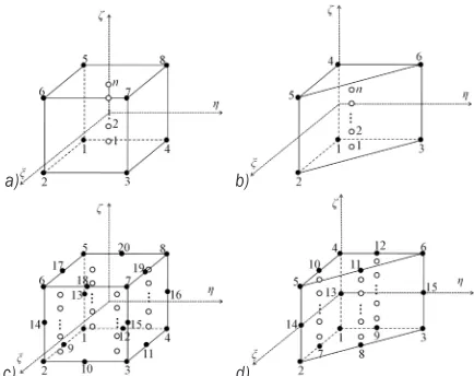
Fig. 1 shows the reference geometry of all SHB elements with the location of their integration points. In the element reference frame, direction ζ denotes the thickness, along which multiple integration points can be used. In general, only two integration points along the thickness direction are sufficient to model elastic problems, while five integration points are recommended for non-linear (elastic–plastic) problems.
a) b)
c) d)
Fig. 1. Reference geometry of the SHB elements and location of their integration points: a) linear hexahedral SHB8PS element; b) linear prismatic SHB6 element; c) quadratic hexahedral SHB20
element, and d) quadratic prismatic SHB15 element
1.2 Quasi-Static Framework
The classical isoparametric linear and quadratic interpolation functions for standard hexahedral and prismatic elements are adopted in the formulation of the SHB elements. Accordingly, the three-dimensional position and displacement of any point inside the element, xi and ui (i = 1, 2, 3) respectively, can be defined using the interpolation functions NI (I = 1, 2, ..., n) as:
x x Ni iI I x NiI I I n =
(
)
=(
)
=∑
ξ η ζ, , ξ η ζ, , , 1 (1)u d Ni iI I d NiI I I n =
(
)
=(
)
=∑
ξ η ζ, , ξ η ζ, , , 1 (2)where xiI and diI denote the Ith nodal coordinate and displacement, respectively. The lowercase subscript i represents the spatial coordinate directions, while n indicates the number of nodes per element.
Next, the discrete gradient operator B defining the relationship between the strain field ∇s
( )
u and the nodal displacement field d is given by:∇s
( )
u = ⋅B d. (3) The SHB element formulation is based on the assumed-strain method, which corresponds to the simplified form of the Hu-Washizu variational principle proposed by Simo and Hughes [18]:π
( )
εε =∫
δεε σσT⋅ −δT⋅ ext=e d
Ω Ω d f 0, (4)
where δ represents a variation, εε the assumed-strain rate, σ the Cauchy stress tensor, d the nodal velocities, and f ext the external nodal forces. The assumed-strain rate εε is defined using a B matrix, which is obtained by projecting the classical discrete gradient operator B
involved in Eq. (3):
εε = ⋅B d. (5)
Inserting Eq. (5) into the variational principle (Eq. (4)), the element stiffness matrix Ke and internal force vector f int can be derived as:
K B C B K
f B
e T ep GEOM
i T e e = ⋅ ⋅ = ⋅
∫
∫
d + d nt Ω Ω Ω Ω , ,σσ (6)
tangent modulus associated with the material behaviour law [19].
In addition to the basic formulation of the SHB elements described above, some special treatments are required for the linear SHB8PS and SHB6 elements in order to improve their performance. In particular, a physical stabilization matrix, computed in a co-rotational coordinate frame [7], is used in the formulation of the SHB8PS element in order to control the zero-energy modes, which are inherent in the reduced-integration technique. Furthermore, an appropriate projection of the strains is required to eliminate some locking phenomena, in particular for the linear SHB6 and SHB8PS elements [7] and [15].
1.3 Explicit/Dynamic Framework
The dynamic version of the SHB elements is essentially based on the quasi-static formulation described above; therefore, it will not be repeated here. However, the mass matrix is required in dynamic problems in order to calculate the inertial term in the variational principle. Note that the stiffness matrix Ke (see Eq. (6)) is not required in such dynamic analysis, except for problems dealing with natural frequency extraction, for which both the stiffness and mass matrix are computed. Several computational methods exist in the literature for the calculation of the element mass matrix [20]. Among them, the lumped mass matrix approach is usually adopted in most dynamic problems, which results in a diagonal mass matrix. In the formulation of the current solid-shell elements, the lumped mass matrix method is followed, due to its computational advantages. Accordingly, the element mass matrix Me (with a size of 3n×3n) can be expressed in terms of the following block of components:
MIJ m N N dI J I J
I J e
= =
≠
∫
ρ ΩΩ
0
, (7)
where m d N N d
e I J e I J
n
=
∫
∑
∫
= =
ρ Ω ρ Ω
Ω Ω
1
. NI and NJ are the element interpolation functions and ρ is the mass density.
2 FINITE ELEMENT SIMULATIONS AND DISCUSSIONS
In this section, several benchmark tests, including both linear and non-linear problems, are selected to evaluate the performance of the SHB solid-shell elements. The first two linear tests are investigated to
examine the convergence rate of the SHB elements. Then, the SHB elements are tested in vibration analysis in order to predict the first four eigenfrequencies of a rectangular cantilever plate and a fully clamped square plate. Finally, three non-linear benchmark problems involving quasi-static and dynamic analyses are carried out to assess the performance of the SHB elements in the framework of large displacements and rotations as well as large strains.
In the following simulations, the geometries are meshed using the nomenclature N1×N2×N3 for the linear and quadratic hexahedral elements (SHB8PS and SHB20), and N1×N2×2×N3 for the linear and quadratic prismatic elements (SHB6 and SHB15), where N1 denotes the number of elements in the length direction, N2 the number of elements in the width direction, and N3 the number of elements in the thickness direction. The latter is equal to 1 in all simulations, which represents a single element layer through the thickness.
2.1 Linear Static Beam Problems
2.1.1 Elastic Cantilever Beam Subjected to Bending Forces
The first linear static test is an elastic cantilever beam with four concentrated loads at its free end. The geometric parameters and material properties are given in Fig. 2. This simple test aims to analyse the behaviour of the SHB elements in the case of bending-dominated conditions. The analytical solution for the deflection at the load point is Uref = 7.326×10⁻³ m. The convergence results are given in Tables 1 and 2 in terms of normalized deflection with respect to the analytical solution. These simulation results prove that all of the SHB elements provide an excellent convergence rate, but with a slower convergence rate for the linear prismatic element SHB6. For the latter, the triangular geometry and the associated interpolation functions lead to constant strain fields inside the element, which requires finer meshes to obtain accurate solutions [15].
Table 1. Normalized deflection results obtained with the linear SHB elements
Mesh SHB8PS Mesh SHB6
U/Uref U/Uref
5×1×1 0.9750 12×2×2×1 0.7062
10×1×1 0.9898 24×2×2×1 0.9019
12×4×1 0.9898 48×2×2×1 0.9669
24×4×1 0.9933 100×4×2×1 0.9807
Table 2. Normalized deflection results obtained with the quadratic SHB elements
Mesh SHB20 Mesh SHB15
U/Uref U/Uref
2×1×1 0.9672 12×2×2×1 0.9896
5×1×1 0.9865 24×2×2×1 0.9925
10×1×1 0.9929
2.1.2 Elastic Cantilever Beam Subjected to Torsion-Type Forces
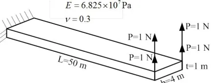
The second linear static test is illustrated in Fig. 3 and consists of a cantilever beam subjected to a torsion-type loading. The end of the beam is loaded by two opposite concentrated forces causing a twisting-type loading along the beam. The geometric and material parameters are given in Fig. 3. In the same way, the deflection results at one load point, normalized with respect to the reference solution Uref = 3.537×10⁻⁴ m, are reported in Tables 3 and 4.
Fig. 3. Elastic cantilever beam subjected to torsion-type loading
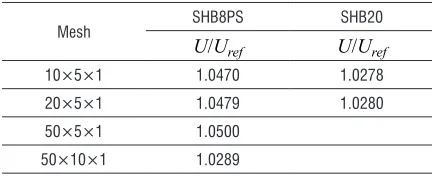
Table 3. Normalized deflection results obtained with the hexahedral SHB elements
Mesh SHB8PS SHB20
U/Uref U/Uref
10×5×1 1.0470 1.0278
20×5×1 1.0479 1.0280
50×5×1 1.0500
50×10×1 1.0289
Table 4. Normalized deflection results obtained with the prismatic SHB elements
Mesh SHB6 SHB15
U/Uref U/Uref
10×5×2×1 0.0107 0.9783
20×5×2×1 0.0247 1.0111
50×5×2×1 0.0916
50×10×2×1 0.3438
100×20×2×1 1.0873
Similar to the previous test problem, the simulation results again show that all of the SHB elements provide a good convergence rate, without noticeable locking phenomena, except for the linear prismatic element SHB6 that requires finer meshes for convergence.
2.2 Plate Vibration Problems
2.2.1 Simple Rectangular Cantilever Plate
The first plate vibration problem is a rectangular cantilever plate with constant thickness. As illustrated in Fig. 4, the rectangular plate, with length L, width b = L/2, and thickness t, is fully clamped on one side, while the other sides are entirely free. The predicted results, in terms of non-dimensional frequency coefficient ω D ρtL4 , associated with the first four
natural frequencies ω are summarized in Table 5, where D E= t3
(
(
− 2)
)
12 1 ν is the flexural rigidity of
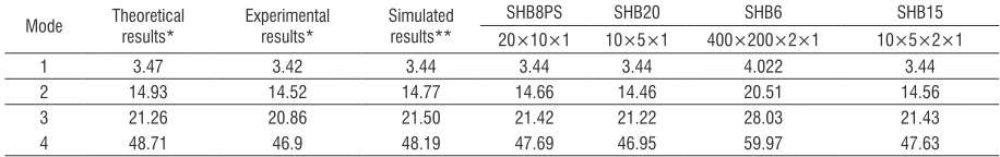
the plate; E and ν are the Young modulus and Poisson ratio, respectively. All predicted results using the SHB8PS, SHB20, and SHB15 elements are in good agreement with the theoretical results as well as with the reference solutions given in [21] and [22]. For the linear prismatic SHB6 element, due to its relatively poor performance, finer meshes are required to obtain relatively accurate solutions.
Fig. 4. Simple rectangular cantilever plate
2.2.2 Fully Clamped Square Plate
length to thickness ratio of this square plate is fixed equal to 1000 and the Poisson ratio of the material is 0.3. For comparison with reference solutions from the literature, the non-dimensional frequency coefficient λ is calculated for the first six natural frequencies of the plate, which is defined as λ2=ω 2 ρ
L t D, where D
is the flexural rigidity defined in the previous test problem. All predicted frequency coefficients obtained using SHB elements are summarized in Table 6 and compared with reference solutions taken from [23]
and [24]. Similar to the previous vibration problem, the obtained results show the performance and efficiency of the SHB elements in determining the natural frequencies of plates, except for the linear prismatic SHB6 element, for which finer meshes are inherently required to obtain accurate results.
Fig. 5. Clamped square plate
2.3 Non-Linear Static Problems
2.3.1 Fully Clamped Circular Plate
A fully clamped elastic circular plate subjected to a uniform pressure is considered here, which involves geometric nonlinearities. The geometric dimensions
Table 5. Natural frequency coefficients for the rectangular cantilever plate
Mode Theoretical
results*
Experimental results*
Simulated results**
SHB8PS SHB20 SHB6 SHB15
20×10×1 10×5×1 400×200×2×1 10×5×2×1
1 3.47 3.42 3.44 3.44 3.44 4.022 3.44
2 14.93 14.52 14.77 14.66 14.46 20.51 14.56
3 21.26 20.86 21.50 21.42 21.22 28.03 21.43
4 48.71 46.9 48.19 47.69 46.95 59.97 47.63
Note: results marked by * are taken from [21], while results marked by ** are available in [22].
Table 6. Natural frequency coefficients for the clamped square plate
Mode Reference solution* Simulated results** SHB8PS SHB20 SHB6 SHB15
16×16×1 16×16×1 400×400×2×1 16×16×2×1
1 5.999 6.024 6.004 6.012 6.659 6.027
2,3 8.567 8.671 8.599 8.605 9.079 8.632
4 10.4 10.52 10.387 10.545 11.337 10.533
5,6 11.5 11.78 11.590 11.523 12.257 11.614
Note: results marked by * are taken from [23], while results marked by ** are taken from [24].
and material elastic properties are taken from [25] and summarized in Fig. 6. Due to the symmetry of the problem, only one quarter of the plate is modelled, which is meshed using 105 SHB8PS elements, 3200 SHB6 elements, 39 SHB20 elements, and 78 SHB15 elements, successively. Fig. 7 shows the numerical results, in terms of the non-dimensional ratio of the central deflection W0 to the thickness t, obtained with the SHB elements together with the reference solution from [25] and the analytical solution given by Chia [26]. As revealed by Fig. 7, all SHB solid‒shell elements provide an accurate solution for this type of bending problem as compared to the reference and analytical solutions.
Fig. 6. Clamped circular plate
2.3.2 Pinched Semi-Cylindrical Shell
of the free circumferential edge, while the other circumferential edge is fully clamped (see Fig. 8 for the geometric and material parameters as well as the remaining boundary conditions). Due to the symmetry of the problem, only one half of the structure is modelled. Fig. 9 displays the load-deflection curves at the load point A, which are obtained using the SHB elements along with the reference solution available
in [27]. The simulation results show good agreement with the reference solution given in [27], which was obtained using (40×40) shell elements. Note, however, that these good convergence results are obtained here with less computational effort, since the SHB elements most often require coarser meshes, except for the linear prismatic SHB6 element, where a finer mesh is required to obtain an accurate solution.
2.4 Explicit Dynamic Problems
2.4.1 Elastic Cantilever Beam Bending
In order to evaluate the dynamic non-linear response of the SHB elements, we consider here an elastic cantilever beam that is loaded impulsively with a concentrated force applied at its free end. The geometric parameters and material properties are summarized in Fig. 10. The deflection history at Point A (indicated at the free edge in Fig. 10), which is obtained with the SHB elements, is plotted in Fig. 11, where it is compared with the reference results given in [8]. From this figure, one can observe that for all of the SHB elements, both the maximum deflection and time period are in good agreement with those provided by the reference solution.
Fig. 10. Elastic cantilever beam under impulsively-applied loading
Fig. 11. Deflection history for the elastic cantilever beam under dynamic loading
Fig. 7. Normalized central deflection results for the clamped circular plate
Fig. 8. Pinched semi-cylindrical shell
2.4.2 Simply Supported Elastic Beam
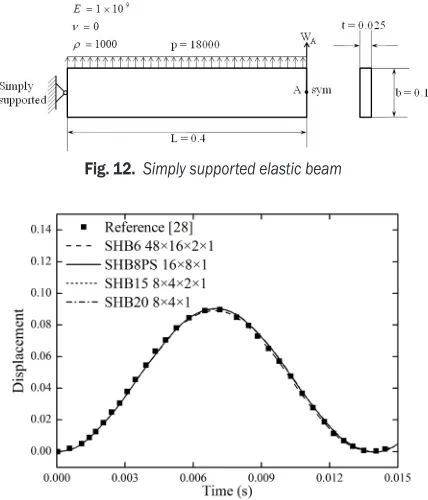
The second non-linear dynamic problem is an elastic beam, which is simply supported at both ends. The beam is subjected to a uniform load, resulting in a maximum deflection of the order of its depth. The geometric dimensions, material properties, and boundary conditions are all summarized in Fig. 12. Owing to the symmetry of the problem, only half of the beam is discretized. The deflection of the central point, obtained with the SHB solid-shell elements, is depicted in Fig. 13 and compared with the reference solution taken from [28]. It can be seen that the numerical results obtained with the proposed SHB elements are in good agreement with the reference solution.
Fig. 12. Simply supported elastic beam
Fig. 13. Deflection results for the simply supported elastic beam
2.5 Application to the Simulation of Deep Drawing Process
In this section, a popular sheet metal forming process, involving geometric and material nonlinearities as well as double-sided contact, is simulated to further evaluate the performance of the proposed SHB elements. This selective benchmark consists in the simulation of the deep drawing process of a cylindrical cup, which is commonly used to study the earing profile of the cup when the anisotropic behaviour of sheet metals is considered. The initially circular metal sheet, with a diameter of 158.76 mm and a thickness of 1.6 mm, is made of an AA2090-T3 aluminium alloy
[29]. For the modeling of the elastoplastic material behaviour, isotropic hardening described by the Swift law is considered. Its expression is given by
σy=k(ε +εeqp n) ,
0 (8)
where σy is the yield stress, εeqp is the equivalent plastic strain, and (k, ε0, n) are the hardening parameters. The Hill’48 quadratic yield criterion is adopted in this work to characterize the anisotropic plasticity of the sheet metal. All of the material parameters are summarized in Tables 7 and 8 [29]. The schematic view and dimensions of the drawing setup are given in Fig. 14.
Table 7. Elastic−plastic parameters for the AA2090-T3 aluminium
sheet
E [MPa] ν k [MPa] ε0 n
70500 0.34 646 0.025 0.227
Table 8. r-values for the AA2090-T3 aluminium sheet
r0 r45 r90
0.2115 1.7695 0.6923
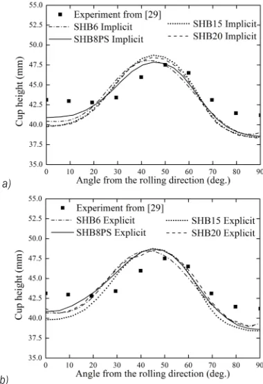
peak value at 50° from the rolling direction, while the predicted cup heights are underestimated at 0° and 90° from the rolling direction. These predictions could be improved in the future by using more appropriate anisotropic yield criteria [29], which can predict more than four earing profiles for the complete circular blank, as observed experimentally for aluminium alloys [30] and [31].
Fig. 14. Schematic view of the drawing setup [29]
a) b)
c) d)
Fig. 15. Final deformed shape for a completely drawn cylindrical cup using a) the SHB8PS elements; b) the SHB6 elements; c) the
SHB20 elements; and d) the SHB15 elements
3 CONCLUSIONS
The assumed-strain solid–shell finite element technology SHB has been extended to explicit dynamic analysis and coupled with advanced anisotropic plasticity models for the modeling of thin three-dimensional structures under quasi-static or dynamic loading conditions and sheet metal forming processes. This family of SHB solid–shell elements consists of a linear 6-node prismatic element and a linear 8-node hexahedral element as well as their quadratic counterparts (15-node prismatic element and 20-node hexahedral element, respectively). All of these linear and quadratic solid–shell elements have been implemented into ABAQUS implicit/static and explicit/dynamic software packages to model various
quasi-static and dynamic problems. The respective capabilities of the proposed SHB elements were first evaluated through a series of linear and non-linear benchmark tests, both in static and dynamic analyses. The obtained results, using only a single element layer with two integration points, showed excellent performance in terms of convergence rate and accuracy when compared to reference solutions yielded by existing state-of-the-art solid and shell finite elements from the literature. Then, the performance of the SHB elements has been assessed via the simulation of the deep drawing process of a cylindrical cup made of an aluminium alloy with anisotropic plastic behaviour. For comparison purposes, both implicit/quasi-static and explicit/dynamic versions of the SHB elements have been used for these deep drawing simulations. The earing profiles predicted by the implicit/quasi-static and explicit/dynamic versions were found to be reasonably close to each other, and in satisfactory agreement with the experiments on the whole. Nevertheless, the prediction of the earing profiles could be improved by adopting advanced non-quadratic anisotropic yield functions that are more suitable to aluminium alloys.
a)
b)
Fig. 16. Predicted cup height profiles obtained by a) implicit/ static and b) explicit/dynamic analysis, along with experimental
4 REFERENCES
[1] Abed-Meraim, F., Combescure, A. (2002). SHB8PS–a new
adaptive, assumed-strain continuum mechanics shell element for impact analysis. Computers & Structures, vol. 80, no. 9-10,
p. 791-803, DOI:10.1016/S0045-7949(02)00047-0.
[2] Parente, M.P.L., Fontes Valente, R.A., Natal Jorge, R.M.,
Cardoso, R.P.R., Alves de Sousa, R.J. (2006). Sheet metal forming simulation using EAS solid-shell finite elements. Finite Elements in Analysis and Design, vol. 42, no. 13, p.
1137-1149, DOI:10.1016/j.finel.2006.04.005.
[3] Reese, S. (2007). A large deformation solid-shell concept
based on reduced integration with hourglass stabilization.
International Journal for Numerical Methods in Engineering,
vol. 69, no. 8, p. 1671-1716, DOI: 10.1002/nme.1827.
[4] Schwarze, M., Reese, S. (2009). A reduced integration
solid-shell finite element based on the EAS and the ANS concept—
Geometrically linear problems. International Journal for
Numerical Methods in Engineering, vol. 80, no. 10, p.
1322-1355, DOI:10.1002/nme.2653.
[5] Caseiro, J.F., Valente, R.A.F., Reali, A., Kiendl, J., Auricchio, F., Alves de Sousa, R.J. (2015). Assumed natural strain NURBS-based solid-shell element for the analysis of large deformation
elasto-plastic thin-shell structures. Computer Methods in
Applied Mechanics and Engineering, vol. 284, p. 861-880,
DOI:10.1016/j.cma.2014.10.037.
[6] Flores, F.G. (2016). A simple reduced integration hexahedral
solid-shell element for large strains. Computer Methods in
Applied Mechanics and Engineering, vol. 303, p. 260-287,
DOI:10.1016/j.cma.2016.01.013.
[7] Abed-Meraim, F., Combescure, A. (2009). An improved
assumed strain solid–shell element formulation with physical stabilization for geometric non-linear applications and elastic–
plastic stability analysis. International Journal for Numerical
Methods in Engineering, vol. 80, no. 13, p. 1640-1686,
DOI:10.1002/nme.2676.
[8] Pagani, M., Reese, S., Perego, U. (2014). Computationally
efficient explicit nonlinear analyses using reduced
integration-based solid-shell finite elements. Computer Methods in
Applied Mechanics and Engineering, vol. 268, p. 141-159,
DOI:10.1016/j.cma.2013.09.005.
[9] Sena, J.I.V., Alves de Sousa, R.J., Valente, R.A.F. (2011). On the use of EAS solid-shell formulations in the numerical simulation
of incremental forming processes. Engineering Computations,
vol. 28, no. 3, p. 287-313, DOI:10.1108/02644401111118150.
[10] Cardoso, R.P.R., Yoon, J.W., Mahardika, M., Choudhry, S., Alves de Sousa, R.J., Fontes Valente, R.A. (2008). Enhanced assumed strain (EAS) and assumed natural strain (ANS) methods for one-point quadrature solid-shell elements.
International Journal for Numerical Methods in Engineering,
vol. 75, p. 156-187, DOI:10.1002/nme.2250.
[11] Ben Bettaieb, A., Velosa de Sena, J.I., Alves de Sousa, R.J., Valente, R.A.F., Habraken, A.M., Duchene, L. (2015). On the comparison of two solid-shell formulations based on in-plane reduced and full integration schemes in linear and non-linear
applications. Finite Element in Analysis and Design, vol. 107,
p. 44-59, DOI:10.1016/j.finel.2015.08.005.
[12] Moreira, R.A.S., Alves de Sousa, R.J., Valente, R.A.F. (2010). A solid-shell layerwise finite element for non-linear geometric
and material analysis. Composite Structures, vol. 92, p.
1517-1523, DOI:10.1016/j.compstruct.2009.10.032.
[13] Naceur, H., Shiri, S., Coutellier, D., Batoz, J.L. (2013). On the modeling and design of composite multilayered structures
using solid-shell finite element model. Finite Elements in
Analysis and Design, vols. 70-71, p. 1-14, DOI:10.1016/j. finel.2013.02.004.
[14] Kpeky, F., Boudaoud, H., Abed-Meraim, F., Daya, E.M. (2015). Modeling of viscoelastic sandwich beams using solid–shell
finite elements. Composite Structures, vol. 133, p. 105-116,
DOI:10.1016/j.compstruct.2015.07.055.
[15] Trinh, V.D., Abed-Meraim, F., Combescure, A. (2011). A new assumed strain solid–shell formulation “SHB6” for the
six-node prismatic finite element. Journal of Mechanical Science
and Technology, vol. 25, no. 9, p. 2345-2364, DOI:10.1007/ s12206-011-0710-7.
[16] Abed-Meraim, F., Trinh V.D., Combescure, A. (2013). New quadratic solid–shell elements and their evaluation on linear
benchmark problems. Computing, vol. 95, no. 5, p. 373-394,
DOI:10.1007/s00607-012-0265-1.
[17] Wang, P., Chalal, H., Abed-Meraim, F. (2015). Efficient solid-shell finite elements for quasi-static and dynamic analyses and their application to sheet metal forming simulation.
Key Engineering Materials, vols. 651-653, p. 344-349, DOI:
10.4028/www.scientific.net/KEM.651-653.344.
[18] Simo, J.C., Hughes, T.J.R. (1986). On the variation foundations
of assumed strain methods. Journal of Applied Mechanics,
vol. 53, no. 1, p. 51-54, DOI:10.1115/1.3171737.
[19] Salahouelhadj, A., Abed-Meraim, F., Chalal, H., Balan, T. (2012). Application of the continuum shell finite element SHB8PS to sheet forming simulation using an extended
large strain anisotropic elastic–plastic formulation. Archive
of Applied Mechanics, vol. 82, no. 9, p. 1269-1290,
DOI:10.1007/s00419-012-0620-x.
[20] Zienkiewicz, O.C., Taylor, R.L., Zhu, J.Z. (2006). The Finite Element Method: Its Basis and Fundamentals, Sixth ed., Elsevier Ltd., Oxford, UK.
[21] Barton, M.V. (1951). Vibration of rectangular and skew
cantilever plates. Journal of Applied Mechanics, vol. 18, p.
129-134.
[22] Anderson, R.G., Irons, B.M., Zienkiewicz, O.C. (1968). Vibration
and stability of plates using finite elements. International
Journal of Solids and Structures, vol. 4, no. 10, p. 1031-1055,
DOI:10.1016/0020-7683(68)90021-8.
[23] Leissa, A.W. (1969). Vibration of Plates. Scientific and Technical Information Division, NASA, Washington, DC, USA.
[24] Sze, K.Y., Yao, L.Q. (2000). A hybrid stress ANS solid-shell element and its generalization for smart structure modelling. Part I: solid-shell element formulation. International Journal for Numerical Methods in Engineering, vol. 48, no. 4, p. 545-564,
DOI:10.1002/(SICI)1097-0207(20000610)48:4<545::AID-ME889>3.0.CO;2-6.
[25] Cai, Y.C., Atluri, S.N. (2012). Large rotation analyses of plate/ shell structures based on the primal variational principle and a fully nonlinear theory in the updated lagrangian
& Sciences, vol. 83, no. 3, p. 249-273, DOI:10.3970/ cmes.2012.083.249.
[26] Chia, C.Y. (1980). Nonlinear analysis of plate, McGraw-Hill, New York, USA.
[27] Sze, K.Y., Liu, X.H., Lo, S.H. (2004). Popular benchmark
problems for geometric nonlinear analysis of shells. Finite
Elements in Analysis and Design, vol. 40, no. 11, p.
1551-1569, DOI:10.1016/j.finel.2003.11.001.
[28] Flanagan, D.P., Belytschko, T. (1981). A uniform strain hexahedron and quadrilateral with orthogonal hourglass
control. International Journal for Numerical Methods in
Engineering, vol. 17, no. 5, p. 679-706, DOI:10.1002/ nme.1620170504.
[29] Yoon, J.W., Barlat, F., Dick, R.E., Karabin, M.E. (2006). Prediction of six or eight ears in a drawn cup based on a new anisotropic yield function. International Journal of Plasticity,
vol. 22, no. 1, p. 174-193, DOI:10.1016/j.ijplas.2005.03.013.
[30] Banabic, D., Barlat, F., Cazacu, O., Kuwabara, T. (2010).
Advances in anisotropy and formability. International Journal
of Material Forming, vol. 3, p. 165-189, DOI:10.1007/s12289-010-0992-9.
[31] Wang, J., Sun, J. (2012). Plane strain transversely anisotropic analysis in sheet metal forming simulation using 6-component
Barlat yield function. International Journal of Mechanics and