R E V I E W
Open Access
Detecting individual ancestry in the human
genome
Andreas Wollstein
1,2*†and Oscar Lao
1,3*†Abstract
Detecting and quantifying the population substructure present in a sample of individuals are of main interest in the fields of genetic epidemiology, population genetics, and forensics among others. To date, several algorithms have been proposed for estimating the amount of genetic ancestry within an individual. In the present review, we introduce the most widely used methods in population genetics for detecting individual genetic ancestry. We further show, by means of simulations, the performance of popular algorithms for detecting individual ancestry in various controlled demographic scenarios. Finally, we provide some hints on how to interpret the results from these algorithms.
Keywords:Population substructure, Human genetic variability, SNPs, Global ancestry, Individual ancestry, ADMIXTURE, fastSTRUCTURE, MDS, PCA, sNMF
Review
Introduction
The genetic variability among the human species is known to be relatively low compared to other primate species [1]. There are paradoxically more genetic differ-ences between Western and Eastern chimpanzee individ-uals sampled in the African continent [2] than in any genome of two human individuals sampled in different continents [3]. Human genetic diversity also tends to be positively correlated with the geographic distance be-tween the sampled individuals [4-6], which is mainly a result from isolation by distance [7]. Studies using clas-sical partition of the human genetic variance based on analysis of molecular variance (AMOVA [8]), and its generalization GAMOVA [9], have consistently shown that a small proportion (approximately 10% to 15%) of the total genetic variability is explained by continent of origin, whereas the majority (approximately 80%) is ex-plained by within-individual variation. The remaining approximately 5% of the genetic variation is explained by the populations [10]. Interpreting these results in terms of human population substructure and individual prediction to a population cluster is still controversial
[11]. Some argue that humans should be considered as one genetically homogeneous group [12]; others suggest that, although small, the geographic dependence of hu-man genetic diversity (at least) supports the existence of continental groups [11,13].
Inferring population substructure in the human gen-ome is cumbersgen-ome and is the main goal for the large number of genetic ancestry algorithms and approaches that have been proposed in the last decade. A basic as-sumption is that any current individual genome or population is a mixture of ancestries from past popula-tions [14]. Therefore, genetic ancestry is defined at dif-ferent scales of complexity: at populations, at individuals within a population, and at a locus within an individual. In the present review, we focus on current methods for inferring genetic ancestry in the genome of an individ-ual. We analyze the performance of some of the most commonly used programs through simulated data and show the range of parameters in which each program provides reliable results in those settings.
Methods for identifying individual ancestry
Methods for estimating ancestry have traditionally fo-cused on populations; their main interests are to estab-lish the relationship among populations and to quantify the admixture proportions in the admixed populations [15,16]. Admixture proportions are computed from the * Correspondence:[email protected];[email protected]
†Equal contributors 1
Department of Forensic Molecular Biology, Erasmus MC University Medical Center Rotterdam, 3000 CA, Rotterdam, The Netherlands
Full list of author information is available at the end of the article
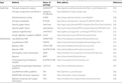
amount of loci that can be traced back to a certain an-cestral population. Population methods are the oldest in literature [17] and are a large number of available appli-cations [18-21]. However, it has been suggested that there could be hidden population substructure among the individuals from an assumed population [22]. The main goal of global individual ancestry methods is to de-scribe the relationship between individuals in terms of genetic ancestry. This can either mean the identification of thea prioriunknown ancestry components, the quan-tification of the proportions of these components, or the identification of the assumed population of an individ-ual. Individual ancestry methods can be classified de-pending on the assumptions of the method, the scope of the algorithms (that is, the whole genome is assigned to one ancestry versus the whole genome is a mixture of ancestries), and the use of prior ancestry information, among others (see Table 1). From a technical point of view, there is large variation in the speed and computa-tional requirements of the different methods [16,23]. Speed depends on the computational complexity of each method which, for example, is O(n m K2) for ADMIX-TURE [24] and O(n m K) for sNMF [25], as well as the possibility to apply divide-and-conquer computational
approaches such as multithreading (for example, in AD-MIXTURE and sNMF). However, multithreading can only provide a linear time factor gain, which in the case of higher polynomial complexities does not have a strong computational impact.
Depending on which methodological approach is used, global individual ancestry methods have been divided by Alexander et al. [24] into algorithmic and model-based methods [24]. We use this classification through the manuscript with some modifications. By definition, all the algorithms are ‘algorithmic’. Therefore, we will use the term ‘model-free’ for referring to the ancestry methods classified by Alexander et al. [24] as algorith-mic, and point out that the use of ‘model’refers here to a population-based statistical model, as further de-scribed. Nevertheless, we acknowledge that some of the newest proposed methods can also be considered as hy-brids of the two classifications or even can be barely assigned to any of them. Model-free methods are based on the use of multivariate techniques [26] such as Prin-cipal component analysis (PCA; [27]) or Multidimen-sional scaling (MDS [28,29]). For a given measured divergence between any pair of sampled individuals, the basic idea behind all these techniques is to represent the
Table 1 Commonly applied algorithms to SNP data for quantifying individual population substructure in humans
Type Method Name of package
Web address Reference
Model-free Principal component analysis EIGENSOFTa http://genetics.med.harvard.edu/reich/Reich_Lab/Software.html [70]
Principal components and Moran’sI adegenet (R software)
http://adegenet.r-forge.r-project.org/ [71]
Multidimensional scaling PLINKa http://pngu.mgh.harvard.edu/~purcell/plink/ [28]
Principal coordinates PCO-MC http://lamar.colostate.edu/~reevesp/PCOMC/PCOMC.html [72]
Spectral graph theory GemTools http://wpicr.wpic.pitt.edu/WPICCompGen/GemTools/GemTools.htm [43]
Spectral graph theory SpectralGem http://wpicr.wpic.pitt.edu/WPICCompGen/Spectral-GEM/GEM+.htm [56]
Laplacian eigenfunction LAPSTRUCT http://galton.uchicago.edu/~junzhang/LAPSTRUCT.html [57]
Genetic algorithm coupled to AMOVA GAGA http://www.erasmusmc.nl/fmb/resources/GAGA/ [73]
Model-based Log-likelihood HWE ADMIXTURE https://www.genetics.ucla.edu/software/admixture/ [24]
Log-likelihood HWE FRAPPE http://med.stanford.edu/tanglab/software/frappe.html [31]
Bayesian HWE STRUCTURE http://pritchardlab.stanford.edu/structure.html [22]
Bayesian HWE fastSTRUCTURE http://pritchardlab.stanford.edu/structure.html [59]
Nonnegative matrix factorization sNMF http://membres-timc.imag.fr/Eric.Frichot/snmf/index.htm [25]
Bayesian BAPS http://www.helsinki.fi/bsg/software/ [74]
Chromopainting and Bayesian classifier
fineSTRUCTURE http://www.paintmychromosomes.com [60]
Log-likelihood genotypic/haplotypic gradients
LOCO-LD http://loco.icsi.berkeley.edu/loco/ [37]
Log-likelihood allelic gradients SPA http://genetics.cs.ucla.edu/spa/ [36]
ADMIXTURE and linear regression GPS http://chcb.saban-chla.usc.edu/gps/ [39]
Bayesian clustering with spatial information
TESS http://membres-timc.imag.fr/Olivier.Francois/tess.html [38]
a
genetic relationships by a new set of orthogonal variables that are ordered by the decreasing amount of explained variation. Both methods can be considered as equivalent if Euclidean distances are used [29]. Visualization of these relationships becomes very meaningful if only the variables with the highest amount of explained variation are considered. Because multivariate methods are ex-ploratory, they do not make any assumption about the underlying genetic model of the data [26]. Nevertheless, in some idealized cases, the proposed coordinates in some of these methods can be interpreted in demo-graphic terms (for example, PCA [30]). In contrast, model-based methods estimate ancestry coefficients as the parameters of a statistical model. This model takes into account basic demographic assumptions, such as the presence of the Hardy-Weinberg equilibrium (HWE; [22]) in the allelic frequencies of the K‘ancestral’ popu-lations that produced the currently observed data [22,24]. For example, in the original definition of individ-ual ancestry provided by STRUCTURE [22], the geno-type g counted as the number of alleles {0,1,2} in a diploid organism at locus jof individuali is modeled as a mixture of the q fractions of the K ancestral popula-tions at the allelic frequencies f. The log-likelihood under the assumption of HWE for all the individuals i and loci j is then computed using the Alexander et al. [24] notation as:
L Qð ;FÞ ¼X i
X
j gijln
X
k qikfkj
!
þ 2−gij
ln X k
qik 1−fkj
!!
Popular methods for estimating the allelic frequencies fin the ancestral populations for all the loci and the an-cestryq proportions in each individual include Bayesian (for example STRUCTURE [22]) and maximum likeli-hood approaches (for example, FRAPPE [31] and AD-MIXTURE [24]).
Recently, new types of global ancestry methods have been proposed. These methods take advantage of the spatial dependence of human population substructure [32] to estimate ancestral geographic coordinates of an individual (BAPS2 [33], GENELAND [34], sPCA [35], SPA [36], LOCO-LD [37], TESS [38], or GPS [39] among others).
There are several ways to estimate the unknown num-ber (K) of ancestral populations from the data (for ex-ample, [40]). In model-based methods, the algorithm is explicitly run by the user at differentKs. The most sup-ported number of clusters or ancestral components is then ascertained by taking the one that optimizes the parameter of performance of the algorithm (for example, it maximizes the log-likelihood of the posterior in the case of STRUCTURE; minimization of cross-validation error is applied in ADMIXTURE among others). In the
case of model-free methods, using their output, a classi-fier algorithm can be applied in order to identify the number of genetically homogeneous population clusters (see for example [41,42], or [43]). One exception is sNMF [25], a new algorithm for inferring ancestry pro-portions. sNMF models the probability of the observed genotypespil in individualiat locuslas a fractionqikof K ancestral genotype probability gkl, similar in spirit as STRUCTURE or ADMIXTURE:
pilð Þ ¼j X K
k¼1
qikgklð Þj
where j =0,1,2 denotes the number of alleles. However, this algorithm does not make any assumption about HWE in the ancestral populations. The corresponding matrix representation is P = QG, where the unknown Q and G can be estimated by nonlinear matrix factorization. This is achieved by means of minimizing two least square criteria:
Ls1¼jX−QGjandLs2¼ GT;
ffiffiffi
α p
1K
QT−XT;0n
;
where alpha is a regularization parameter, and 1k and 0n
describe a column vector with ones and zeros of size K andn(see [25] for further details; the semicolon indicates a line break). Starting from random matrices as initial condition, the algorithm applies both criteria consecu-tively to obtain estimates about Qfrom Ls1and G from
Ls2, respectively, until convergence has been reached.
Since model-based methods explore the space of pos-sible solutions starting from an initial point, it is recom-mended to run the algorithm several times at different initial starting points for each proposedKand to check for reproducibility of results [44]. Different strategies have been proposed for combining the results from dif-ferent runs. One possibility is to compute a consensus ancestry value by merging all the solutions [44]. Another is just to take the run that provides the best value of model performance [24].
Usually, investigators apply both model-free (for ample, PCA or MDS) and model-based methods (for ex-ample, ADMIXTURE, FRAPPE, or STRUCTURE) to the same dataset [45,46]. Plots (and further interpretation) tend to include the solutions of the optimal/best sup-ported number of clusters.
Ups and downs of individual genetic ancestry estimation Individual ancestry methods can depict a detailed pic-ture of the genetic landscape of human populations [15]. Furthermore, these algorithms are routinely applied to any dataset before conducting a genome-wide associ-ation study (GWAS), in order to correct for the putative presence of hidden population substructure [48]. More-over, they have been used to test the hypothesis of the ancestry origin of the perpetrator at a crime scene in fo-rensic cases [49].
In principle, averaging the fragments of local ancestry over the genome of one individual computes the global ancestry estimation in that individual; similarly, aver-aging all of the global individual ancestries in one popu-lation provides a migration/admixture estimation in that population. Moreover, the mean and variance in the length of the ancestry fragments and the global ancestry proportions can be used to estimate parameters such as the time or migration rate of the admixture event in particular demographic scenarios [50]. Nevertheless, population-based methods are sometimes preferred over global or local ancestry methods [18,51]. The main reason is that the results of global and local ancestry methods can be particularly difficult to interpret [21,52]. For example, several demographic scenarios can produce the same observed admixture pattern in PCA [30,53,54]. In humans, multiple demographic events can be identified in the same geographic area [55]; therefore, it is likely to find anad hocplausible planation for any estimated admixture pattern (for ex-ample, see [53]). The presence of unequal sample size of the (a prioriunknown) populations can also bias the output of some algorithms, such as PCA [30,56]; the presence of highly genetically related individuals and gen-etic outliers can also bias the output from different
algorithms (such as in the case of PCA, [57]). Further-more, the outcome from the different algorithms can dif-fer substantially even for the same dataset [58]. Ultimately, there is the question of what a proposed‘ancestral popula-tion’ is. By definition, since new populations appear by splitting from previous ones, population ancestry (and hence genetic admixture) can be defined at different time scales, taking into account that all individuals from a spe-cies ultimately share a common ancestral origin. However, this population‘birth and death’process is not really mod-eled in the model-based methods (and by default, neither is it in the model-free methods); in contrast, it is one of the main goals of population-based methods, conditioned to the proper definition of‘what a current population is’.
We exemplify some of these caveats using unsupervised analyses from four ascertained global-based algorithms on simulated and real data using the default parameter set-tings from each algorithm. In particular, we consider AD-MIXTURE [24], sNMF [25], fastSTRUCTURE [59], PCA [27], and MDS in PLINK [28]. This selection is based on methodological, historical, and computational characteris-tics. For example, we did not consider fineSTRUCTURE [60], a recently developed algorithm with enhanced power for detecting population substructure [61], because of its computational burden when the number of SNPs and sampled individuals are large (see the manual of fineS-TRUCTURE and chromoPainter for details). The first two methods represent model-based algorithms. ADMIX-TURE [24] is a maximum likelihood algorithm. It can be considered the gold standard of model-based methods; it is relatively fast and allows for the use of a large number of SNPs and samples. fastSTRUCTURE is a new software that implements a Bayesian framework similar to STRUC-TURE [22]. However, in contrast to STRUCSTRUC-TURE, fas-tSTRUCTURE allows the fast analysis of a large number
of samples and SNPs. PCA, MDS, and sNFM are model-free methods. PCA and MDS are based on eigenvalue de-composition. They produce almost identical results in real data [62,63]; therefore, we have used either one or the other indistinctly in the different simulations. sNMF [25] is a novel software which in principle produces very simi-lar results to ADMIXTURE [24] but at a computationally faster speed.
We focused our analyses on two simple, controlled, demographic models. The first demographic model de-scribes an ancestral population that splits t generations ago in two populations. In one version of the model, the two descendent populations start evolving independ-ently. In another version, migration between the two populations is allowed. The second model comprises an ancestral population that splits in two, which after a certain number of generations evolving with a genetic barrier, create a new population by admixture (see Figure 1). Because of their simplicity, the proposed demographic models fit better into the assumptions of model-based methods. Furthermore, it has been shown that the first dimension of the PCA can differentiate the genetic ancestry of populations, and it is indicative of the ancestry proportions in the admixed populations [30]. In our analyses, we used markers in linkage equilib-rium; this condition was either imposed on the simulator (case of ms simulations) or achieved by the use of com-monly applied LD pruning techniques. Therefore, any difference observed in the estimated ancestry propor-tions must reflect inner algorithmic assumppropor-tions or sen-sitivity to the modification of the considered parameters.
Performance of global-based algorithms to estimate genetic ancestry on two simulated populations
Two populations with a genetic barrier
The results from the two-population model (Figure 1A) with a genetic barrier and the details of the implementa-tion are shown in Tables 2 and 3.
Table 2 Default parameter used in two-population models, with and without migration
Parameter Abbreviation Default value
Sample size population 1 n1 100
Sample size population 2 n2 100
Number of independent SNPs nsnps 5,000
Mutation rate (length)a theta 2
Effective population sizeb N1, N2 10,000
Divergence time T1 2,000
Constant migration rate 4Nm 0
a
The scaled mutation rate theta = 2*Ne*mu= 2 describes a region of about 2 kb assuming a mutation rate of 2.5e−8.b
The effective population size corresponds broadly to that of Africa.
Table 3 Results from the two-population model simulations
Variable sNMF (R2)
Admixture (R2)
fastStructure (R2)
Sampling depth, n1, n2
8 99.92 100 39.56
10 99.83 100 34.03
20 99.87 100 100
40 99.81 100 100
100 99.74 100 100
Uneven sampling, n1
8 98.94 99.45 98.59
10 99.43 99.78 99.32
20 99.61 100 92.21
40 99.67 100 100
100 99.74 100 100
Sequencing depth, nsnps
10 3.13 0.65 18.51
50 66.56 75.54 74.42
100 85.33 92.95 91.89
500 96.78 99.87 99.93
1,000 98.62 99.99 100
5,000 99.74 100 100
Population size, theta
1 99.73 100 100
2 99.74 100 100
5 99.74 100 100
10 99.72 100 100
Effective population size, N2
100 99.98 100 100
2,500 99.94 100 100
7,500 99.82 100 100
10,000 99.74 100 100
Divergence time (Fst),
T/(4 N1)
0.000075 0.54 0.38 0.01
0.00025 0.24 0.03 0
0.00125 6.19 0.03 0.24
0.0025 69.36 95.28 0.53
0.0125 98.36 100 100
0.05 99.74 100 100
Constant migration rate, 4Nm
0.1 99.77 100 100
1 99.78 100 100
Overall, sNMF and ADMIXTURE show similar results and outperform fastSTRUCTURE for most of the con-sidered demographic values (see Table 4). Nevertheless, the predictive power of ADMIXTURE is slightly higher than that of sNMF (100% compared to 99% in most cases). Low sample size decreases the power mostly in fastSTRUCTURE (for n= 8, fastSTRUCTURE: 35%, sNMF: 99%, ADMIXTURE: 100%), whereas uneven sam-pling does not influence the estimates of the ancestry components with any of the programs. The number of SNPs has a strong impact on all programs. When only very few sites are available (that is, less than 50 snps), fastSTRUCTURE produces the best outcome. This is not surprising, as ADMIXTURE and sNMF have been particularly developed to consider a dense number of markers [25]. The effective population size and differ-ences in population size did not show any direct impact on the results, which however might matter in combin-ation with divergence time. The power for all programs decreases dramatically for populations that do not ex-hibit substantial population subdivision due to low diver-gence times or high migration rates, mostly for fastSTRUCTURE. Reliable ancestry estimates are pos-sible for t> 0.0125 that correspond to Fst>0.0124 [64]. The counter effect of constant migration becomes evi-dent for a migration rate of 4Nm >10 (see Figure 2B), which homogenizes the population. Sampling more sites is likely to increase the sensitivity to detect both effects.
Migration between the two descendent populations (continuous gene flow model)
In addition, we studied the parameter range where mi-gration becomes detectable depending on the start time and rate of migration in the continuous gene flow (CGF) model (see Figure 1A for the model and Figure 2 for re-sults). Keeping the migration rate fixed at high migration rate (4Nm =2,000), the populations become distinguish-able if the migration starts before 100 generations back-ward in time (Figure 2B). Beyond that value, the effect of migration is so strong that the two populations appear
to be panmictic. In contrast, when fixing the start time of migration at ten generations, we observe that all populations become recognizable by all programs for 4 Nm <500. The estimated proportions of ancestry do not match the proportion of migrants over time. A Table 3 Results from the two-population model
simulations(Continued)
10 99.15 99.99 100
50 93.95 99.98 33.3
100 41.61 94.06 0.56
We simulated two populations using ms [75], which splitted and evolved independentlytgenerations ago. See Table1for default parameters. Each simulation comprises 1,000 independent regions of 2 kb, from which one SNP per region is sampled at random. Each parameter set was replicated ten times. For each algorithm, the estimated ancestry proportions over the different runs were sorted according to the expected ancestry matrix denoting the true population labels using CLUMPP [44]. From this, standard denoted demographic parameters were successively varied to exemplify the impact on the estimates. We report the coefficient of determination that can be understood as the percentage of the true outcome.
Table 4 Results from admixture simulation with changing parameter in the HI model from HapMap III data
Parameter sNMF (R2) ADMIXTURE (R2) fastSTRUCTURE (R2)
Sample size
8 98.2 99 86.66
10 99.5 99.52 98.69
20 99.74 99.82 99.71
40 99.85 99.9 99.86
50 99.87 99.93 99.9
100 99.91 99.95 99.95
nsnps
5 4.56 15.38 19.44
10 15.92 47.37 46.2
50 80.62 86.31 86.89
100 89.67 93.04 93.33
500 98.46 99.07 99.11
1,000 99.19 99.54 99.56
5,000 99.84 99.92 99.91
10,000 99.91 99.95 99.95
Nbreaks
5 88.82 88.37 87.46
10 94.38 94.86 94.43
50 98.74 98.87 98.8
100 99.33 99.41 99.38
500 99.81 99.85 99.84
1,000 99.86 99.91 99.9
5,000 99.91 99.94 99.94
10,000 99.91 99.95 99.95
alpha
0.01 99.94 99.99 99.99
0.03 99.93 99.97 99.95
0.07 99.93 99.97 99.92
0.1 99.93 99.97 99.91
0.3 99.91 99.96 99.95
0.5 99.91 99.95 99.95
possible reason is that there is a continuous gene flow from one population into the other so that recombin-ation has not enough time to produce the homoge-neous mosaic of ancestral fragments that is emerging from the HI model (see below). Therefore, the migra-tion rate cannot be inferred from this analysis.
We further investigated how the presence of hidden in-breeding affects the estimated genetic ancestry proportions from each algorithm. We used the two-population model with constant migration (4Nm =100) as previously de-scribed. In each simulation, a fraction of heterozygote ge-notypes was decreased proportional to theFis(for example, [65]) by replacing them by random homozygote genotypes in one population. We estimated the genetic ancestry by the different programs (see Figure 3 for results). The mi-gration has a homogenizing effect on the genetic variation in both populations, whereas the inbreeding in one of the populations results in the opposite pattern. For low Fis
values (Fis< 0.1), we observe that sNMF and fastSTRUC-TURE indicate correctly the effect of migration in their es-timates (see Figure 3). In contrast, for highFisvalues (Fis> 0.1), the genetic variation is more divergent in sNMF and fastSTRUCTURE; in contrast, both populations appear more similar with ADMIXTURE. Therefore, sNMF and fastSTRUCTURE seem to provide better ancestry esti-mates compared to ADMIXTURE, particularly when in-breeding is high (Fis> 0.1). If migration is absent, inbreeding has a minor effect on the ancestry estimates from the different algorithms (data not shown).
For completeness, we studied the running time per-formance of each algorithm as a function of the number of considered SNPs and for either K= 2 or K= 4 as-sumed ancestral populations (see Figure 4). We observed that sNMF shows the lowest running times for a given number of SNPs and K, followed by ADMIXTURE. In contrast, fastSTRUCTURE exhibits the worst runtime
and scaling with higher K as expected from the com-plexity described above.
Performance of the algorithms on the hybrid admixture (HI) model
Simulated data
Analyses focused on the estimated individual ancestry proportions in the hybrid population using the HI
model (Figure 1B). We compared them with the real proportions of genomic admixture in each individual; this measure was estimated for each simulation by tra-cing back the ancestry of the genomic fragments that compose the genome of each admixed individual to ei-ther of the two parental populations. Therefore, in con-trast to other approaches, which produce admixed individuals in forward generations from sampled real populations (that is, African Americans have been modeled as a mixture of CEU and YRI individuals from HapMap III [66]; also see the next section), we avoid the artificial introduction of strong bottlenecks.
As seen in Figure 5, the error of the estimated ances-try proportions differ based on the software, the amount of genetic differentiation present among the parental populations, and the ratios of sampled individ-uals between the parental populations. With the same number of sampled individuals by parental population, ancestry proportions estimated by fastSTRUCTURE show the largest deviation to the real ancestral propor-tions in all the simulapropor-tions. In all cases, admixture pro-portions in the admixed population tend to be better estimated if the parental populations are genetically dif-ferentiated (Fst> 0.1); nevertheless, even in that case, the mean difference between the estimated and the real admixture proportion can reach 5% in the case of sNMF and MDS, and 6% in the case of fastSTRUC-TURE. Unequal sample sizes of the parental popula-tions also affect the performance of the different algorithms. ADMIXTURE and fastSTRUCTURE show a systematic error bias in the estimation of the admix-ture proportions in the hybrid population when there is unequal sample size in the parental populations, inde-pendently of the amount of population differentiation among the parental populations.
Figure 4Netto time estimates for fastSTRUCTURE, sNMF, and ADMIXTURE.Mean time estimates of the termination of the respective programs from ten independent replications. We simulated 100 chromosomes from two populations with an effective population size of 10,000 and aNe*m= 20 using ms [75] (see legend of Figure 2 for command details). The termination time can be expected to scale similarly as the number of used SNPs given the complexity of the programs.
Real data from HapMap III data
Simulations from synthetically generated admixed popu-lations from African (YRI) and European (CEU) as an-cestral populations were produced (see Table 4 for results and clarification of the applied methodology). We use the number of breakpoints to mimic the time of ad-mixture [14] and sampled SNPs with a minimum dis-tance of 1 Mb to ensure linkage equilibrium. The results for sample size, number of SNPs, and admixture time, represented here as the number of breaks, are quite similar to the two-population simulations above. The
power of sNMF and ADMIXTURE is quite comparable. fastSTRUCTURE loses power more rapidly with lower sample size and maintains a better power for low num-bers of SNPs. All programs have an equally high power to estimate the ancestry components.
Conclusions
Identifying hidden population substructure in the gen-ome of an individual is important for a number of scien-tific disciplines. So far, the proposed algorithms are invaluable tools for detecting and controlling for the
Figure 5Estimated error in the estimated individual admixture proportions from the simulated admixed population (HI model).We used an extended version of the backward demographic simulator described in [76] that includes recombination and different types of mating and allows for ancestry painting [14]. Over all parameters that are defined in this model [19], we varied the time of split of the ancestral populations, which ranged between 50 and 2,000 generations among simulations. Each simulation generated 75 (25 by population) full human genomes with 22 diploid chromosomes (l) with the following sizes: 13.65, 13.15, 11.20, 10.65, 10.20, 9.65, 9.35, 8.50, 8.40, 8.95, 7.95, 8.65, 6.35, 5.80, 6.30, 6.75, 6.50, 5.95, 5.40, 5.40, 3.10, and 3.65 Mb [77]. The mutation rate was set to 2.5 × 10⁻⁸[78] and the recombination rate to 1.8 × 10⁻⁸. PLINK was applied to exclude SNPs with minor allele frequency less than 0.05 and LD (default PLINK–indep 50 5 2). The effective population sizes of the parental and hybrid populations were set to 5,000 diploid individuals; the time of admixture was ten generations ago, and each parental population equally contributed to the admixed population. By this way, we minimized the putative effect of genetic drift in the admixture proportions of the hybrid population. Furthermore, in order to include the effects of bias sample size, we repeated all the analyses with 1:1(A)
presence of hidden population substructure. In the sim-plest demographic models, these methods can also be used to estimate demographic parameters. However, inter-preting the output of each algorithm from an evolutionary point of view can be difficult. Different demographic sce-narios can lead to the same ancestry estimates, and differ-ent estimates can be retrieved when applied to the same dataset. Extrapolating the results from our simple simula-tions to real data (that is, suggesting which is the best al-gorithm) can be misleading; except for cases such as the admixture of European and Sub-Saharan African popula-tions in the US [67], admixture usually involves more than two parental populations (for example, Latin America, al-though see [68]). In addition, parental populations tend to show a non-negligible gene flow [61] with admixed popu-lations that can substantially differ in the effective popula-tion size compared to the parental populapopula-tions (for example, see the European Romani [46]), while usually the parental populations are unknown.
The number of SNPs and sample size seem to be a limiting factor in all the algorithms that we have tested; therefore, it would be recommended to use as many markers (conditioned in the absence of LD when re-quired by the algorithm) and samples as possible. How-ever, in our simple model, we observe already good estimates for >10 samples and >1,000 markers. In case fewer markers are available, fastSTRUCTURE provides the best estimates followed by ADMIXTURE and sNMF. Furthermore, it is recommendable to run more than one algorithm on the same data at the same time given the observed diversity of results, different sensitivity to biased sample size of the different algorithms, and an-cestry noise. In this sense, combining global anan-cestry and population ancestry methods (for example, [69]), or using the output from these algorithms as summary sta-tistics [40], can improve the identification of population substructure. Finally, although they can be used to pro-vide hypotheses about the origin and evolution of popu-lations, it is recommended to test the evolutionary hypotheses by means of other methods [46], rather than providing an ad hoc interpretation; in particular, any demographic interpretation from these methods should be further validated by means of demographic simula-tions, showing that the proposed demographic model can produce the observed output of genetic ancestry.
Abbreviations
AMOVA:Analysis of molecular variance; CGF: Continuous gene flow model; GAMOVA: Generalized analysis of molecular variance; GWAS: Genome-wide association study; HWE: Hardy-Weinberg equilibrium; MDS: Classical multidimensional scaling, also called principal coordinate analysis; PCA: Principal component analysis; SNP: Single nucleotide polymorphism.
Competing interests
The authors declare that they have no competing interests.
Authors’contributions
AW and OL participated in the design of the study and performed the statistical analyses. AW and OL equally participated in the drafting of the manuscript. Both authors read and approved the final manuscript.
Acknowledgements
This study was funded in part by the Erasmus University Medical Center Rotterdam. AW was additionally supported by Volkswagen Foundation (ref 80462). We would like to thank Susan Walsh and Wolfgang Stephan for helpful comments on the manuscript.
Author details
1
Department of Forensic Molecular Biology, Erasmus MC University Medical Center Rotterdam, 3000 CA, Rotterdam, The Netherlands.2Section of Evolutionary Biology, Department of Biology II, University of Munich, 82152 Planegg-Martinsried, Germany.3Current address: Centro Nacional de Análisis Genómico, Baldiri Reixac, 4, Barcleona Science Park - Tower I, 08028 Barcelona, Spain.
Received: 13 October 2014 Accepted: 12 January 2015
References
1. Cavalli-Sforza LL. Human evolution and its relevance for genetic epidemiology. Annu Rev Genomics Hum Genet. 2007;8:1–15.
2. Chimpanzee Sequencing and Analysis Consortium. Initial sequence of the chimpanzee genome and comparison with the human genome. Nature. 2005;437:69–87.
3. Barbujani G, Colonna V. Human genome diversity: frequently asked questions. Trends Genet. 2010;26:285–95.
4. Handley LJL, Manica A, Goudet J, Balloux F. Going the distance: human population genetics in a clinal world. Trends Genet. 2007;23:432–9. 5. Ramachandran S, Deshpande O, Roseman CC, Rosenberg NA, Feldman MW,
Cavalli-Sforza LL. Support from the relationship of genetic and geographic distance in human populations for a serial founder effect originating in Africa. Proc Natl Acad Sci U S A. 2005;102:15942–7.
6. Rosenberg NA. Algorithms for selecting informative marker panels for population assignment. J Comput Biol. 2005;12:1183–201.
7. Jay F, Sjödin P, Jakobsson M, Blum MGB. Anisotropic isolation by distance: the main orientations of human genetic differentiation. Mol Biol Evol. 2013;30:513–25.
8. Excoffier L, Smouse PE, Quattro JM. Analysis of molecular variance inferred from metric distances among DNA haplotypes: application to human mitochondrial DNA restriction data. Genetics. 1992;131:479–91. 9. Nievergelt CM, Libiger O, Schork NJ. Generalized analysis of molecular
variance. PLoS Genet. 2007;3:e51.
10. Lewontin RC. The apportionment of human diversity. In: Evolutionary biology. US: Springer; 1995. p. 381–98.
11. Edwards AWF. Human genetic diversity: Lewontin’s fallacy. Bioessays. 2003;25:798–801.
12. Barbujani G. Human races: classifying people vs understanding diversity. Curr Genomics. 2005;6:215–26.
13. Risch N. Dissecting racial and ethnic differences. N Engl J Med. 2006;354:408–11.
14. Pugach I, Matveyev R, Wollstein A, Kayser M, Stoneking M. Dating the age of admixture via wavelet transform analysis of genome-wide data. Genome Biol. 2011;12:R19.
15. Novembre J, Ramachandran S. Perspectives on human population structure at the cusp of the sequencing era. Annu Rev Genomics Hum Genet. 2011;12:245–74.
16. Liu Y, Nyunoya T, Leng S, Belinsky SA, Tesfaigzi Y, Bruse S. Softwares and methods for estimating genetic ancestry in human populations. Hum Genomics. 2013;7:1.
17. Bernstein F. Die geographische Verteilung der Blutgruppen und ihre anthropologische Bedeutung. 1932.
18. Pickrell JK, Pritchard JK. Inference of population splits and mixtures from genome-wide allele frequency data. PLoS Genet. 2012;8:e1002967. 19. Bertorelle G, Excoffier L. Inferring admixture proportions from molecular
data. Mol Biol Evol. 1998;15:1298–311.
21. Patterson N, Moorjani P, Luo Y, Mallick S, Rohland N, Zhan Y, et al. Ancient admixture in human history. Genetics. 2012;192:1065–93.
22. Pritchard JK, Stephens M, Donnelly P. Inference of population structure using multilocus genotype data. Genetics. 2000;155:945–59. 23. Yang B-Z, Zhao H, Kranzler HR, Gelernter J. Characterization of a
likelihood based method and effects of markers informativeness in evaluation of admixture and population group assignment. BMC Genet. 2005;6:50.
24. Alexander DH, Novembre J, Lange K. Fast model-based estimation of ancestry in unrelated individuals. Genome Res. 2009;19:1655–64. 25. Frichot E, Mathieu F, Trouillon T, Bouchard G, François O. Fast and efficient
estimation of individual ancestry coefficients. Genetics. 2014;196:973–83. 26. Jombart T, Pontier D, Dufour A-B. Genetic markers in the playground of
multivariate analysis. Heredity. 2009;102:330–41.
27. Patterson N, Price AL, Reich D. Population structure and eigenanalysis. PLoS Genet. 2006;2:e190.
28. Purcell S, Neale B, Todd-Brown K, Thomas L, Ferreira MAR, Bender D, et al. PLINK: a tool set for whole-genome association and population-based linkage analyses. Am J Hum Genet. 2007;81:559–75.
29. Cox TF, Cox M. Multidimensional scaling. 2nd ed. New York: Chapman & Hall/CRC; 2010.
30. McVean G. A genealogical interpretation of principal components analysis. PLoS Genet. 2009;5:e1000686.
31. Tang H, Peng J, Wang P, Risch NJ. Estimation of individual admixture: analytical and study design considerations. Genet Epidemiol. 2005;28:289–301. 32. Novembre J, Johnson T, Bryc K, Kutalik Z, Boyko AR, Auton A, et al. Genes
mirror geography within Europe. Nature. 2008;456:98–101.
33. Cheng L, Connor TR, Sirén J, Aanensen DM, Corander J. Hierarchical and spatially explicit clustering of DNA sequences with BAPS software. Mol Biol Evol. 2013;30:1224–8.
34. Guillot G, Mortier F, Estoup A. Geneland: a computer package for landscape genetics. Mol Ecol Notes. 2005;5:712–5.
35. Jombart T, Devillard S, Dufour A-B, Pontier D. Revealing cryptic spatial patterns in genetic variability by a new multivariate method. Heredity. 2008;101:92–103.
36. Yang W-Y, Novembre J, Eskin E, Halperin E. A model-based approach for analysis of spatial structure in genetic data. Nat Genet. 2012;44:725–31. 37. Baran Y, Quintela I, Carracedo A, Pasaniuc B, Halperin E. Enhanced
localization of genetic samples through linkage-disequilibrium correction. Am J Hum Genet. 2013;92:882–94.
38. Chen C, Durand E, Forbes F, François O. Bayesian clustering algorithms ascertaining spatial population structure: a new computer program and a comparison study. Mol Ecol Notes. 2007;7:747–56.
39. Elhaik E, Tatarinova T, Chebotarev D, Piras IS, Maria Calò C, De Montis A, et al. Geographic population structure analysis of worldwide human populations infers their biogeographical origins. Nat Commun. 2014;5:3513. 40. Evanno G, Regnaut S, Goudet J. Detecting the number of clusters of
individuals using the software STRUCTURE: a simulation study. Mol Ecol. 2005;14:2611–20.
41. Fraley C, Raftery AE. Model-based clustering, discriminant analysis, and density estimation. J Am Stat Assoc. 2002;97:611–31.
42. Lawson DJ, Falush D. Population identification using genetic data. Annu Rev Genomics Hum Genet. 2012;13:337–61.
43. Klei L, Kent BP, Melhem N, Devlin B, Roeder K. GemTools: a fast and efficient approach to estimating genetic ancestry. http://arxiv.org/abs/1104.1162. Accessed 10 June 2014.
44. Jakobsson M, Rosenberg NA. CLUMPP: a cluster matching and permutation program for dealing with label switching and multimodality in analysis of population structure. Bioinformatics. 2007;23:1801–6.
45. Wollstein A, Lao O, Becker C, Brauer S, Trent RJ, Nürnberg P, et al. Demographic history of Oceania inferred from genome-wide data. Curr Biol. 2010;20:1983–92.
46. Mendizabal I, Lao O, Marigorta UM, Wollstein A, Gusmão L, Ferak V, et al. Reconstructing the population history of European Romani from genome-wide data. Curr Biol. 2012;22:2342–9.
47. Price AL, Tandon A, Patterson N, Barnes KC, Rafaels N, Ruczinski I, et al. Sensitive detection of chromosomal segments of distinct ancestry in admixed populations. PLoS Genet. 2009;5:e1000519.
48. Tian C, Gregersen PK, Seldin MF. Accounting for ancestry: population substructure and genome-wide association studies. Hum Mol Genet. 2008;17:R143–50.
49. Kayser M, de Knijff P. Improving human forensics through advances in genetics, genomics and molecular biology. Nat Rev Genet. 2011;12:179–92. 50. Verdu P, Rosenberg NA. A general mechanistic model for admixture
histories of hybrid populations. Genetics. 2011;189:1413–26.
51. Pickrell JK, Patterson N, Barbieri C, Berthold F, Gerlach L, Güldemann T, et al. The genetic prehistory of southern Africa. Nat Commun. 2012;3:1143. 52. Kalinowski ST. The computer program STRUCTURE does not reliably identify
the main genetic clusters within species: simulations and implications for human population structure. Heredity. 2011;106:625–32.
53. Novembre J, Stephens M. Interpreting principal component analyses of spatial population genetic variation. Nat Genet. 2008;40:646–9. 54. François O, Currat M, Ray N, Han E, Excoffier L, Novembre J. Principal
component analysis under population genetic models of range expansion and admixture. Mol Biol Evol. 2010;27:1257–68.
55. Sokal RR, Oden NL, Walker J, Di Giovanni D, Thomson BA. Historical population movements in Europe influence genetic relationships in modern samples. Hum Biol. 1996;68:873–98.
56. Lee AB, Luca D, Klei L, Devlin B, Roeder K. Discovering genetic ancestry using spectral graph theory. Genet Epidemiol. 2010;34:51–9.
57. Zhang J, Niyogi P, McPeek MS. Laplacian eigenfunctions learn population structure. PLoS One. 2009;4:e7928.
58. Barbujani G, Belle EMS. Genomic boundaries between human populations. Hum Hered. 2006;61:15–21.
59. Raj A, Stephens M, Pritchard JK. fastSTRUCTURE: variational inference of population structure in large SNP data sets. Genetics. 2014;197:573–89. 60. Lawson DJ, Hellenthal G, Myers S, Falush D. Inference of population
structure using dense haplotype data. PLoS Genet. 2012;8:e1002453. 61. Hellenthal G, Busby GBJ, Band G, Wilson JF, Capelli C, Falush D, et al. A
genetic atlas of human admixture history. Science. 2014;343:747–51. 62. Li JZ, Absher DM, Tang H, Southwick AM, Casto AM, Ramachandran S, et al.
Worldwide human relationships inferred from genome-wide patterns of variation. Science. 2008;319:1100–4.
63. Jakobsson M, Scholz SW, Scheet P, Gibbs JR, VanLiere JM, Fung H-C, et al. Genotype, haplotype and copy-number variation in worldwide human pop-ulations. Nature. 2008;451:998–1003.
64. Nielsen R, Mountain JL, Huelsenbeck JP, Slatkin M. Maximum-likelihood estimation of population divergence times and population phylogeny in models without mutation. Evolution. 1998;52:669–77.
65. Weir BS, Cockerham CC. Estimating F-statistics for the analysis of population structure. Evolution. 1984;38:1358–70.
66. International HapMap 3 Consortium, Altshuler DM, Gibbs RA, Peltonen L, Altshuler DM, Gibbs RA, et al. Integrating common and rare genetic variation in diverse human populations. Nature. 2010;467:52–8. 67. Yaeger R, Avila-Bront A, Abdul K, Nolan PC, Grann VR, Birchette MG, et al.
Comparing genetic ancestry and self-described race in African Americans born in the United States and in Africa. Cancer Epidemiol Biomarkers Prev. 2008;17:1329–38.
68. Bryc K, Auton A, Nelson MR, Oksenberg JR, Hauser SL, Williams S, et al. Genome-wide patterns of population structure and admixture in West Africans and African Americans. Proc Natl Acad Sci U S A.
2010;107:786–91.
69. Reich D, Patterson N, Campbell D, Tandon A, Mazieres S, Ray N, et al. Reconstructing Native American population history. Nature. 2012;488:370–4. 70. Price AL, Patterson NJ, Plenge RM, Weinblatt ME, Shadick NA, Reich D.
Principal components analysis corrects for stratification in genome-wide association studies. Nat Genet. 2006;38:904–9.
71. Jombart T. adegenet: a R package for the multivariate analysis of genetic markers. Bioinformatics. 2008;24:1403–5.
72. Reeves PA, Richards CM. Accurate inference of subtle population structure (and other genetic discontinuities) using principal coordinates. PLoS One. 2009;4:e4269.
73. Lao O, Liu F, Wollstein A, Kayser M. GAGA: a new algorithm for genomic inference of geographic ancestry reveals fine level population substructure in Europeans. PLoS Comput Biol. 2014;10:e1003480.
74. Corander J, Waldmann P, Marttinen P, Sillanpää MJ. BAPS 2: enhanced possibilities for the analysis of genetic population structure. Bioinformatics. 2004;20:2363–9.
75. Hudson RR. Generating samples under a Wright–Fisher neutral model of genetic variation. Bioinformatics. 2002;18:337–8.
skin-color variation from tests based on SNP scans and resequencing. Investig Genet. 2011;2:24.
77. Gravel S. Population genetics models of local ancestry. Genetics. 2012;191:607–19.
78. Nachman MW, Crowell SL. Estimate of the mutation rate per nucleotide in humans. Genetics. 2000;156:297–304.
Submit your next manuscript to BioMed Central and take full advantage of:
• Convenient online submission
• Thorough peer review
• No space constraints or color figure charges
• Immediate publication on acceptance
• Inclusion in PubMed, CAS, Scopus and Google Scholar
• Research which is freely available for redistribution