Volume 20, Number 1, pp. 71–82. http://www.scpe.org
ISSN 1895-1767 c
⃝2019 SCPE
A PARTICLE SWARM OPTIMIZATION BASED LOAD SCHEDULING ALGORITHM IN CLOUD PLATFORM FOR WIRELESS SENSOR NETWORKS
ARVINDA KUSHWAHA∗AND MOHD AMJAD†
Abstract. Integration of wireless sensor network into cloud computing is a growing paradigm that supports a massive amount of applications in cloud computing, optimization of resources required in the machines. This integration requires the optimization of resources to efficiently complete the different tasks in the devices at cloud platform. This optimization can be done using load scheduling algorithms. These algorithms reduce overload and achieve higher throughput by maximizing the machine utilization concerning cost stabilization. There are lots of methods like First Come First Serve, Min-Min, Particle Swarm Optimization (PSO) for optimizing the load but we use Particle Swarm Optimization as it obtains the motivation from the social behavior of the flock of birds and analyses various approaches for load scheduling. In this paper, we propose the load scheduling algorithm based on PSO in wireless sensor networks for cloud computing to minimize total transfer time and cost stabilization. The proposed method is compared with the existing approaches used for load scheduling in Cloudlets. It is clear from the simulation results that the proposed method is more efficient because it minimizes the transfer time and cost than the conventional algorithms thereby making a system for cost stable.
Key words: Wireless Sensor Networks, Particle Swarm Optimization, Load Scheduling, Cloudlets, Cloud Computing.
AMS subject classifications. 68Q25, 68R10, 68U05
1. Introduction. The Wireless Sensor Networks (WSNs) have seen significant growth in academia as well as the industry in the field of WSNs due to the advancement in the sensor’s abilities like sensing power, computation, and communication capabilities, in last decade and so. WSNs possess different characteristics like energy constraints, fault tolerance, heterogeneity and homogeneity of nodes, deployment scalability, ease of use, and adaptability to sustain in extreme environmental conditions [1, 2]. In WSN, various sensors are spread in the target area for supervising and logging the physical conditions of the environment that have a small size, low processing power, less storage, and low energy abilities. These sensor nodes can sense the target and make an infrastructure-less wireless communication among them and base station (BS). Sensors accumulate the data from the target area and forward it to the BS directly or with the assistance of other sensors. The BS is connected to the cloud server with the help of wired/wireless links. Thus, the information is accessed by the users from the cloud servers [3]. The BS is supposed to be reliable and is capable of performing any operation. WSNs are being used in different applications like battlefield surveillance, data centre monitoring and data logging, health care supervision, forest fire detection, landslide detection, natural disaster prevention, water quality monitoring, structural health monitoring, environmental conditions such as extreme temperature variation, sound, pollution levels, humidity, wind, etc., industrial and consumer applications like monitoring of computer system health, industrial process supervision and control etc., and so on [4]. On the bases of the above-discussed applications, the wireless sensor node deployment can be categorized into two categories like deterministic and non-deterministic. In deterministic deployments, sensor nodes are placed into controlled manner or manually at the selected locations where the deployment area is physically accessible such as city sense monitoring, soil monitoring, etc. On the other hand, in non-deterministic deployments sensor nodes are deployed into physically inaccessible areas using other sources like sensors are dropped from an aircraft, e.g., battlefield surveillance and landslide detection, etc. The non-deterministic deployment is also called random deployment [5, 6].
Due to the widespread advent of the Internet of Things (IoT) which connects daily use objects such as mobile devices, Smart TVs, washing machines, Air conditioners, etc. to the internet so that an intelligent linking can be done. Therefore, the user of the devices can communicate with the tools as per his/her convenience being either at home or office. One of the essential parts of the Internet of Things paradigm is wireless sensor networks (WSNs). To expand the wireless services with the online user base, there is a need of efficient hosting of the aggregated data from WSN on the cloud which is very flexible and cost-effective solution, so that online user
∗Department of Computer Engineering, Jamia Millia Islamia, New Delhi, India, ID ([email protected]) †Department of Computer Engineering, Jamia Millia Islamia, New Delhi, India, ID (([email protected])
can intelligently and efficiently communicate [7].
So, in this paper, we introduce a cost-efficient architecture for hosting the WSN data on the cloud platform. The architecture uses PSO based scheduling algorithm for load balancing among the servers of cloud so that the cost and time can be minimized.
This paper is framed in the following manner. The literature review of the integration techniques of wireless sensor networks and cloud computing is discussed in 2. A system model that includes the assumption for wireless sensor networks and cloud, network model is presented in 3. The proposed algorithmic method including flowchart is discussed in 4. The experimental setup and results are presented in 5. Finally,the paper provides the conclusions in 6.
2. Literature Review. In this section, we will discuss the literature review based on the integration of cloud platform and wireless sensor networks.
In paper [14], authors discuss an integrating framework for cloud paradigm and WSNs, which use data processability and cloud service model entirely. In the frame, data are efficiently utilized and managed to form the WSN by considering different information services provided to the users. In paper [15], an author discusses different types of scheduling algorithms and compares their results with various parameters. It also shows the many limitations of the existing algorithms such as they have not considered the execution time for calculating the performance of the method.
In paper [16], a trust assisted sensor cloud system is discussed which focuses on improving the quality of service of sensor cloud for users to obtain sensory data from the cloud. In faith supported sensor cloud system, trusted sensors which have trust values more significant than a threshold, collect and transmit sensory data to the cloud. Then the cloud selects the trusted data centers, which have trust values more significant than a threshold, to store, process the sensory data and further transmit the processed sensory data to users on demand. They show the trust assisted sensor cloud system can substantially improve the response time for users to obtain sensory data from the cloud system and compared to without faith supported sensor cloud system. In paper [17], the authors discussed wireless sensor network packet simulator, server application and web service, developed at the Institute Mihajlo Pupin for storing and viewing data collected by the network. The paper [18] discusses a novel architecture based on cloud computing for improving the performance of WSNs. In this architecture, a cloud platform acts as a virtual sink with the base station that collects data from sensors and processed in the distributed manner in the cloud system.
The paper [19] discusses an extensible and flexible architecture for integrating WSNs with the Cloud called REST. The REST-based Web services are used as an interoperable application layer that can be directly integrated into other application domains for remote monitoring. The paper [20] discusses a data processing framework for transmitting desired data to the mobile users. It decreases the storage requirements for sensor nodes and networks gateway and minimizes the traffic overhead and bandwidth requirement. However, the framework can able to predict the future trends of the sensory data and provides security for this sensory data. The paper [23] analyzes the characteristics of job scheduling concerning integration cloud computing and wireless sensor networks and then discusses two popular job scheduling algorithms namely Min-Min and Max-Min. Two scheduling algorithms are proposed with the integration of cloud computing and wireless sensor networks by considering the Min-Min, and Max-Min and results of the proposed algorithms show shorter expected completion time than Min-Min and Max-Min, for cloud computing integrated with WSN. The paper [24] shows the optimal computing node searched in a limited time by proposing an ant colony algorithm. Three timers were used in setting back time for three role ants such as information and, positioning ant and task ant. When timer started, the general node of WSN was in power saving state. It takes a shorter time for the optimal computing resource. The paper [25] discusses location sleep scheduling algorithm with load balancing (LCLSS) scheme. It considers both awake and asleep status of sensors dynamically. It performs scheduling purely by mobile users current location. It reduces the power consumption and applies to remove areas applications where replacement of the battery is quite difficult. In the next section, we will discuss the system model and the assumptions for the integration of cloud computing and wireless sensor networks.
• All nodes have similar capabilities, energy heterogeneity, location unaware, memory and computation constraints; a unique ID recognizes each node.
• The base station is stationarily located at the center in the network, and the sensor battery recharge or replacement is not possible.
• Each node has the capability to aggregate data, and the received signal strength can calculate the distance between nodes.
• The radio link consumes same energy in transmission and receiving information thus these links called symmetric connections.
• WSNs transmit gathered data to the cloud and end users require sensory data from the cloud.
• Multiple data centers are considered which consist of numerous data server in the cloud.
This network model consists of 3-types of classes based on their initial energy. In this network, WSN has n nodes out of which φ∗nnodes have minimum energy, where a range ofφis 0≤φ≥1. We call these nodes Class-1 nodes and their energy is denoted as E1. The φ2
∗nnodes have more energy than the Class-1 nodes, call these nodes Class-2 nodes and their energy is denoted as E2. The remaining nodes have maximum energy called Class-3 nodes, i.e., (n-(φ*n+φ2*n)) andE3denotes their energy. The sensor nodes have maximum energy
considered to be minimum in numbers. The total energy of the network (T otalenergy) is given below:
T otalenergy=φ∗n∗E1+φ2∗n∗E2+ (1−φ−φ2)∗n∗E3 (3.1) This model describes a WSN, i.e., consisting of Class-1, Class-2, and Class-3 heterogeneity by considering the value of model parameter φ. The range of φ is between 0 and 1. When we put φ=0 in (3.1), it gives one non-zero term which contains only Class-3 nodes. It indicates the 1-level of heterogeneity, but these nodes have E3 energy. In the case of 1-level heterogeneity, appropriate constraints are imposed to haveClass-1 nodes instead of the Class-3 nodes. It may be calculated by defining the following equation:
φ= E3−E1
N∗f(E2, E3) (3.2)
whereN andf are the positive integer greater than 1 and the function ofE2andE3, respectively. The function has either (E3+E2) or (E3-E2). In (3.2), the value ofφshould be in the consonant by considering the constraint:
E1< E2< E3.
The 2-level of heterogeneity contains two type of nodes, i.e., Class-1 and Class-2 for this we need to find the value ofφby considering the following equation:
1−φ−φ2= 0 (3.3)
Equation (3.3) is generated by (3.1) by considering the third term which generates the two level of heterogeneity. We call these nodes Class-1 and Class-2 nodes. Equation (3.3) has two solutions: ((√5)-1)/2 and ((√5)+1)/2. Sinceφis upper-bounded by 1 and ((√5)+1)/2>1, the valid solution of (3) is ((√5)-1)/2. Forφ=((√5)-1)/2, the model (1) consists of two types of nodes with energiesE1 andE2.
In the case of 3-level heterogeneity, the range ofφis firstly determined where the upper limit is ((√5)-1)/2. Let the lower limit ofφbeφL that is to find out. The range ofφfor 3-level heterogeneity isφL<φ<((
√
5)-1)/2. Takingf as (E3-E2) andφfrom (3.2), we have
φL<
E3−E1
N∗(E3−E2)<((
√
5)−1)/2 (3.4)
LetE2=α1 +E1 andE3=α2+E2. From (3.4), we have
α2 α1 <
1
n∗θL−1
Or−α2 α1 ≥
1 1−n∗θL
(3.5)
Since L.H.S. of inequality (5) is negative, we should have 1-N*φL <0. This gives 1
The (3.4) can be written as
(E3−E1)≤N∗ ( √
5)−1
2 ∗(E3−E2) (3.7)
This inequality may be written as
N∗((√5)−1)∗E2−2∗E1≤(N∗((√5)−1)−2)∗E3 (3.8)
This model describes WSNs which consists of three types of nodes, i.e., Class-1, Class-2, and Class-3. The total energy of the network (1) also describes the 1-level, 2-level, and 3-level of heterogeneity. In the next section, we will discuss the proposed clustering method for the heterogeneous network model.
4. Proposed Method. In this section, we discuss the proposed method which is divided into two parts namely energy efficient clustering protocols for WSNs and load scheduling algorithm based on PSO for cloud computing.
4.1. Energy Efficient Clustering Protocol For Sensor Networks. In this section, we consider an energy efficient heterogeneous DEEC protocol in WSNs [1]. The 3-level heterogeneous network model consists of three types of sensor nodes which are Class-1, Class-2, and hetDEEC-1, hetDEEC-2 denote Class-3 and its implementation, and hetDEEC-3, respectively. The cluster head selection of [1] assumes N*poptas the average number of cluster heads as in every iteration, and each sensor node assumes the responsibility of a cluster head once in every ri=1/popt iteration, where popt is an initial probability of each sensor node, andri is iteration. The networks average energy E (r)can be calculated as follows:
E(r) = 1
N
N
∑
i=1
Ei(r) (4.1)
where Ei(r) is residual energy. The average probability of ith node for becoming the cluster head during rth iteration can be calculated as follows:
pi =popt[1−
E(r)−Ei(r)
E(r) ] =popt∗
Ei(r)
E(r) (4.2)
The count of cluster heads per iteration is given by
N
∑
i=1 pi=
N
∑
i=1 popt∗
Ei(r)
E(r) =popt N
∑
i=1 Ei(r)
E(r) =N∗popt (4.3)
The cluster head in rthiteration for theith node is given by (using (4.2))
ri= 1
pi
= E(r)
popt∗Ei(r)
=ropt∗
E(r)
Ei(r) (4.4)
As discussed in (3.1), the total energy at the beginning of the sensor network isN∗(φ*E1+φ2*E2+(1-φ-φ2)*E3)
which is increased byφ+φ2*E2/E1+(1-φ-φ2)*E3/E1. Here, all nodes assume the responsibility of cluster head
exactly once in every 1
popt *(φ+φ
2*E2/E1 +(1-φ-φ2 )*E3/E1 )iteration. Thus, the average number of cluster
heads per iteration is(φ+φ2*E2/E1 +(1-φ-φ2 )*E3/E1 )*N*p
class−1. In1-level of heterogeneity, each Class-1 node becomes a cluster head once in every (φ+φ2*E2/E1 +(1-φ-φ2 )*E3/E1) iteration, each Class-2 node
becomes a cluster head (1+α) times more than the Class-1 nodes in every ((φ+φ2*E2
E1 +(1-φ-φ
2)*E3
E1) iteration,
and each Class-3 node becomes a cluster head (1+β) times more than the Class-1 nodes in every ((φ+φ2*E2/E1
+(1-φ-φ2 )*E3/E1 )) iteration. These methods mainly associate weights to obtain the optimal probability for
[1]. The weighted probabilities of the Class-1, Class-2, and Class-3 nodes denoted by pclass−1, pclass−2, and
pclass−3, respectively, are given by
pclass−1=
popt∗Ei(r)
(φ+φ2∗E2/E1+ (1−φ−φ2)∗E3/E1)∗E(r) (4.5)
pclass−2=
popt∗(1 +α)∗Ei(r)
(φ+φ2∗E2/E1+ (1−φ−φ2)∗E3/E1)∗E(r) (4.6)
pclass−3=
popt∗(1 +β)∗Ei(r)
(φ+φ2∗E2/E1+ (1−φ−φ2)∗E3/E1)∗E(r) (4.7)
The cluster head selection probability is calculated as follows.
T(s) = popt
1−popt.(rmod∗1/popt)
if s∈G (4.8a)
= 0otherwise
The thresholds T(si) Class-1, Class-2, and Class-3 nodes are given by
T(si) = pclass−1
1−pclass−1∗(rmod∗1/pclass−1)
if pnrm∈G ′
(4.9a)
= pclass−2
1−pclass−2∗(rmod∗1/pclass−2)
if padv∈G ′′
= pclass−3
1−pclass−3∗(rmod∗1/pclass−3)
if psup∈G ′′′
= 0otherwise
whereG′,G′′ andG′′′ are set of Class-1, Class-2, and Class-3 nodes that have not become cluster heads within last 1
pClass−1 ,
1
pClass−2 ,and
1
pClass−3 rounds, respectively.
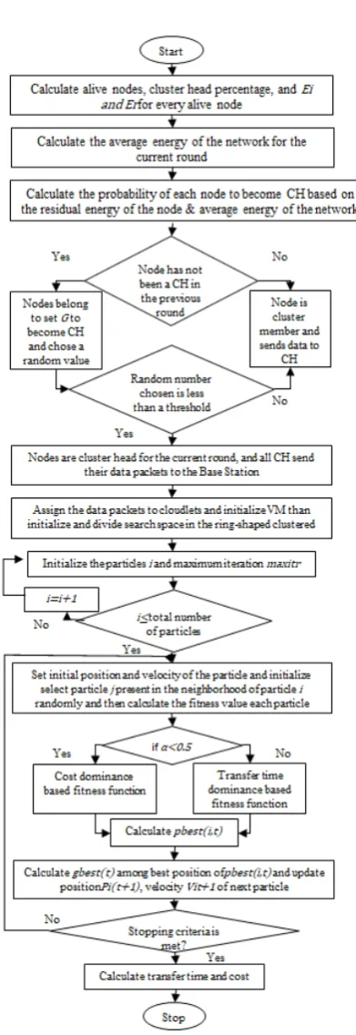
4.2. Load Scheduling Algorithm Based On Particle Swarm Optimization For Cloud Com-puting. In this subsection, we discuss the proposed scheme for load scheduling which is based on simple and basic particle swarm optimization [8, 9]. A new fitness function is incorporating in the proposed method. The proposed scheme defines the fitness function by the transfer time and costs with the higher exploitation of the space of the particles in the base station (BS). The data packets are initialized to the cloudlets and the virtual machines from the BS. The cloudlets are passed to the particles (Np) to be allocated to the optimal virtual machines. The Cost(T) is specified as the total cost of all the tasks are assigned to calculate the resources available. The Cost(T) is calculated as follows:
Cex(T)j =∑ k
Wkj (4.10)
∀T(k) =j (4.11)
Ctotal(T)j=Cex(T)j+Ctr(T)j (4.12)
Cost(T) = max(Ctotal(T)j)∀j∈P (4.13)
HereCex(T)j,Ctr(T)j, andCtotal(T)jare the execution time, the transfer time employed in passing the particles from one resource to another, and gives the sum of the execution cost and the transfer cost between the tasks and the resources for the particle j, respectively. The transfer time is the maximum time taken by all the VMs to complete a particular task. The transfer time is calculated as:
Evmtime(T)k=∑ k
Wk (4.15)
T ransT ime(T) = max (Evmtime(T)k)∀j ∈N (4.16)
k= 1, .., N (4.17)
The new fitness function for both the cost and transfer time parameters is minimized by considering the weights in the system. The new fitness function is calculated as follows.
α∗(Cost(T)) + (1−α)∗T ransT ime(T) (4.18)
min(α(Cost(T)) + (1−α)T ransT ime(T)) (4.19) whereαis the random parameter range from 0 to 1. It is used to shift the load scheduler to both the parameters, i.e., cost and transfer time giving the weightage to both the parameters of the packets in the base station.
The proposed fitness function minimizes weighted sum of transfer time and cost. If the value of α <0.5, higher weightage to the cost function otherwise, higher weightage to the transfer time. The ring-shaped clusters are employed in the neighborhood of the particle to obtain a new global best. The cumulative best values of the clusters help in moving the particles further to the next position.
These motivate in finding the best particles among all the particles, i.e., pbest(i,t) and global best among all the particles in the current iteration, i.e., gbest(t) values.The pbest value is computed as follows:
pbest(i, t) =arg min
k=1,....t[f(Pi(k))], i∈1, ...Np (4.20) and gbest is known as the best position:
gbest(t) =arg min
i=1,....Np;k=1,....t[f(Pi(k))] (4.21) Here, i, Np, f, P, t represent the index of the particle, a total number of particles, symbolically-represent the fitness function, position, and current round/iteration, respectively. The velocity and position of the particles are computed in the following manner.
Vi(t+ 1) =ωVi(t) +c1r1(pbest(i, t)−Pi(t)) +c2r2(gbest(t)−Pi(t)) (4.22)
Pi(t+ 1) =Pi(t) +Vi(t+ 1) (4.23)
where the velocity of the particle i at iteration t is denoted byVi(t), the velocity of the particle i at (t+1 )round is denoted as Vi(t+ 1). The c1 andc2represent the acceleration coefficients of the system & r1 andr2 denote the random values in the range 0 to 1with ω denoting the inertia weight. The best location of the particle i is denoted by pbest(i,t) and the best position among all pbest(i,t) values is generated by gbest(t). The Pi(t) specifies the current position of the particle i at iteration t andPi(t+ 1) denotes the position of the particle i at (t+1) iteration.On the basis of these values, the particles migrate to the next locationPi(t+ 1). The positions of the VMs assigned to the particles are returned for further execution to the cloudlets in the cloud over the datacenter which further schedule the packets in the base station. These values are returned back to the base station.
Fig. 4.1.Proposed Algorithm.
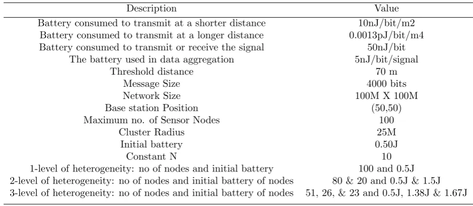
Table 5.1
Simulation parameters for the radio dissipation model and network model for wireless sensor networks [1,3,4]
Description Value
Battery consumed to transmit at a shorter distance 10nJ/bit/m2
Battery consumed to transmit at a longer distance 0.0013pJ/bit/m4
Battery consumed to transmit or receive the signal 50nJ/bit
The battery used in data aggregation 5nJ/bit/signal
Threshold distance 70 m
Message Size 4000 bits
Network Size 100M X 100M
Base station Position (50,50)
Maximum no. of Sensor Nodes 100
Cluster Radius 25M
Initial battery 0.50J
Constant N 10
1-level of heterogeneity: no of nodes and initial battery 100 and 0.5J 2-level of heterogeneity: no of nodes and initial battery of nodes 80 & 20 and 0.5J & 1.5J 3-level of heterogeneity: no of nodes and initial battery of nodes 51, 26, & 23 and 0.5J, 1.38J & 1.67J
The proposed method and existing PSO algorithm [8, 9, 10, 11] are implemented in the CloudSim tool package. The CloudSim is used to perform, designing and analyzing the results and provides users built-in environment. It was given by Garg et al. in 2011, and Network CloudSim Simulator is simulated on top of the CloudSim tool package [7]. We consider two important matrices namely transfer time (seconds) and cost (dollars) for comparing the results of the proposed and existing approaches. The proposed method uses a JSwarm package to perform the simulation. The work in consideration takes ten particles referring to VMs. Each particle’s resources include the following parameters like inertia, maximum & minimum position, and velocity. The dynamic allocation of resources depends on the number of iterations. The iterations taken into consideration are 10, 50, 100, 200, 500, and 1000 in figures. The values are provided before running to the system. The cloudlets and VMs possess the same capability given by the system such as MIPS, transfer cost, execution cost (which are used for the computation of the execution cost and transfer cost), and bandwidth. The parameters supplied to the simulator or the workload characteristics are MIPS (1000), ram (2048), bandwidth (10000), storage (10000) along with the number of iterations.
The results of the proposed method and existing approaches are analyzed by considering two matrices, i.e., transfer time and cost and compared. Six values of the proposed method are considered for the categorization namely, minimum value (α= 0), average value (α= 0.3), best value (α = 0.4), mid or half value (α= 0.5), random value (α= 0.7) and maximum value (α= 1) values. These results are shown for a large set of iterations regarding transfer time and cost concerning the number of iterations.
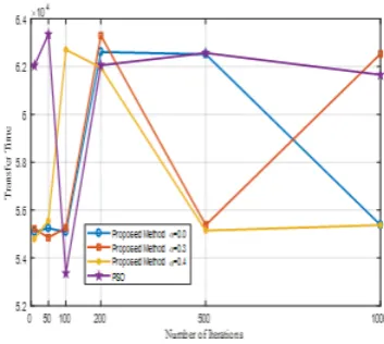
The results are analyzed graphically as given in Fig. 5.1 to 5.4. Fig. 5.1 provides a precise depiction of the transfer time of the proposed approach at various α values, viz., α = 0, α = 0.3, α= 0.4 (best value), respectively with existing ones PSO. Fig. 5.2 shows the current approaches with proposed method along with the various interval values regarding the total transfer time incurred over the number of iterations at α= 0.5 (average value), α= 0.7, α= 1. Finally, it balances the system and decreases the cost of computation as well as the finish time.
Fig. 5.1.Shows the transfer time concerning the number of iteration for the existing PSO and proposed a method by considering the different value ofα=0.0,0.3,and 0.4.
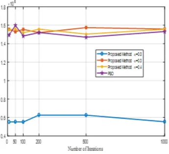
Fig. 5.3 provides a representation of the cost of the proposed method concerning many iterations at different
α values, viz., α= 0, α= 0.3, α= 0.4 (best value), respectively with existing ones PSO. Fig. 5.4 illustrates cost over the number of iterations at α = 0.5 (Average Value), α= 0.7, α= 1. The cost analysis provides much better results for a large number of iterations. The average cost at all the iterations is quite similar. The proposed method gives a stable view of the cost incurred in the system thereby creating a stabilized system. Thus, the proposed approach produces better results regarding transfer time with a stable cost, i.e., no increase in cost. Fig. 5.3 and 5.4 give the total cost differentiation for a larger value of iterations showing maximum optimization. It explains that cost differentiation generates optimal results at various values and best result at
Fig. 5.2. Shows the transfer time concerning the number of iteration for the existing PSO and proposed the method by
considering the different value ofα=0.5,0.7,and 1
Fig. 5.3.Shows the cost for the number of iteration for the existing PSO and proposed a method by considering the different
value ofα= 0.0,0.3and 0.4
It is evident from the Figs. 5.1 to 5.3 that the proposed method takes less transfer time concerning many iteration in the computation of the tasks. It leads to a further reduction in the total computational cost of the system. It produces much higher exploitation of the resources as compared to the existing approaches as evident from the figure. The figure signify the reduction in the total transfer time and total cost based on the proposed method. The cost and transfer time are the prime metrics to justify the storage, processing, and retrieval of data. Lesser transfer time leads to faster processing of user requests. Less cost specifies higher bandwidth and ram for more data processing. This proposed method provides more considerable significance in the real world scenario by optimal allocation, scheduling, and execution of the user requests on the virtual machines. Based on this the total cost incurred in the storage and processing of the data or information in the cloud is further reduced considerably by more considerable search space exploitation.
Table 5.2 shows the network lifetime regarding rounds by taking an equal number of nodes (i.e., 100) and the same amount of total network energy (i.e., 100J) 1-level, 2-level, 3-level heterogeneity. Categorization of nodes and their respective energies are given in details in Table 5.1. The number of rounds for 1-level (Class-1), 2-level (Class-2), 3-level (Class-3) heterogeneity are 2961, 3323, and 4404 in hours, respectively.
Fig. 5.4.Shows the transfer time concerning the number of iteration for the existing PSO and proposed a method by considering
the different value ofα= 0.5,0.7and 1
Table 5.2
Number of rounds for Class-1, Class-2, Class-3 using 100 number of nodes and 100 J network energy for 1-level, 2-level, and 3-level heterogeneity.
Classes Nature of Networks No. of Rounds (hrs) Class-1 1-level heterogeneity 2961
Class-2 2-level heterogeneity 3323 Class-3 3-level heterogeneity 4404
by the computational values viz. the fitness value of the method. The proposed method produces better results and also provides additional benefits by making the system more stable regarding cost. The proposed method achieves higher cost optimization than the existing contemporary PSO based approaching terms of transfer time and thereby making the system more stable on the cost basis. The transfer time and the cost are reduced comparatively at α= 0.4 (Best Value) as shown in the Figures. The future work aims at minimizing the price further to obtain greater feasibility of the results in a cloud computing environment.
REFERENCES
[1] S. Singh and A. Malik ”hetDEEC: Heterogeneous DEEC Protocol for Prolonging Lifetime in Wireless Sensor Networks,” Journal of Information and Optimization Sciences, vol. 38, no. 5, pp. 699-720, 2017.
[2] S. Singh, Energy Efficient Multilevel Network Model for Heterogeneous WSNs Int. Journal Engineering Science and Technol-ogy, vol. 20, no. 1, pp. 105-115, 2017.
[3] A. Malik and S. Singh ”hetSEP: Heterogeneous SEP Protocol for Increasing Lifetime in WSNs,” Journal of Information and Optimization Sciences, vol. 38, no. 5, pp. 721-743, 2017.
[4] S. Singh and A. Malik, Energy Efficient Scheduling Protocols for Heterogeneous WSNs International Journal of Forensic Computer Science, vol. 11, no. 1, pp. 8-29, 2016.
[5] A. Malik and S.Singh, ”HeterogeneousEnergy Efficient Protocol for Enhancing the Lifetime in WSNs I.J. Information Tech-nology and Computer Science, vol.8, no.9, pp. 62-72, 2016.
[6] S. Chand, S. Singh, and B. Kumar, ”Multilevel Heterogeneous Network Model for Wireless Sensor Networks,” Telecommuni-cation Systems, vol. 64(2), pp. 259277, 2016.
[7] S.K. Garg, and R. Buyya, ”Network CloudSim: Modelling Parallel Applications in Cloud Simulations,” 4th IEEE/ACM International Conference on Utility and Cloud Computing (UCC 2011, IEEE CS Press, USA), Melbourne, Australia, 2011.
[8] J Kennedy and R Eberhart, Particle swarm optimization. IEEE International Conference on Neural Networks, 4, 19421948, 1995.
[10] R.Buyya, S Pandey and Vecchiola, Cloudbus toolkit for market-oriented cloud computing.CloudCom 09: Proceedings of the 1st International Conference on Cloud Computing, 2009.
[11] P.Y. Yin, S.S. Yu, and Y.T. Wang, ”A hybrid particle swarm optimization algorithm for optimal task assignment in distributed systems” Computer Standards and Interfaces, 28(4), 441450, 2006.
[12] S. Singh, S. Chand, and B. Kumar, ”Performance Evaluation of Distributed Protocols Using Different Levels of Heterogeneity Models in Wireless Sensor Networks,” Int. Journal of Computer Network and Information Security, 7(1), pp.38-45, 2015. [13] A K Sharma, and S. Singh, Distributed Algorithms for Maximizing Lifetime of WSN with Heterogeneity and Adjustable Range for Different Deployment Strategies I. J. Information Technology and Computer Science, 5(8), pp.101-108, 2013. [14] P. You; Y. Peng; and H. GaoProviding Information Services for Wireless Sensor Networks through Cloud Computing IEEE
Asia-PacificServices Computing Conference (APSCC), pp. 362 - 364, 6-8 Dec. 2012
[15] A.VenumadhavA Survey of Various Workflow Scheduling Algorithms in Cloud Environment International Journal of Scientific and Research Publications, Vol. 3, Issue 10, Oct. 2013.
[16] C. Zhu, V. C. M. Leung, L. T. Yang, L. Shu, J. J. P. C. Rodrigues, X. Li, ”Trust Assistance in Sensor-Cloud” IEEE INFOCOM 2015, pp. 342-347, 2015.
[17] L. Kraus, M. Starcevic, M. Oklobdija and . Stojkovic, ”Integrated Software Tools for Support of Wireless Sensor Network Applications”, 19th Telecommunications forum TELFOR 2011 Serbia, Belgrade, pp. 1289-1292, November 22-24, 2011. [18] P. Zhang, Z. Yan, and H. Sun, ”A Novel Architecture Based on Cloud Computing for Wireless Sensor Network” Proceedings
of the 2nd International Conference on Computer Science and Electronics Engineering (ICCSEE 2013), pp. 472-475, 2013. [19] R. Piyare, S. Park, S. Y. Maeng, S. H. Park, S. C. Oh, Sang G. Choi, H. S. Choi, and S. R. Lee, ”Integrating Wireless Sensor
Network into Cloud Services for Real-time Data Collection” ICTC 2013, pp. 752-756, 2013.
[20] C.M Sukanya et al., ” Integration of Wireless Sensor Networks and Mobile Cloud- a Survey” International Journal of Computer Science and Information Technologies, vol. 6, no. 1, 159-163, 2015.
[21] Y. Singh, S. Singh, and R. Kumar A Distributed Energy-Efficient Target Tracking Protocol for Three Level Heterogeneous Sensor Networks, International Journal of Computer Applications, 51(11), pp-31-36, Aug. 2012.
[22] A K Sharma, and S. Singh Distributed Energy-Efficient Algorithm for Wireless Sensor Networks, International Journal of Advanced Research in Computer Science, 2(3), pp-548-550, June 2011.
[23] C. Zhu, X. Li, V. C. M. Leung, X. Hu, and L. T. Yang, ”Job Scheduling for Cloud Computing Integrated with Wireless Sensor Network,” IEEE 6th International Conference on Cloud Computing Technology and Science, pp. 62-69, 2014
[24] H. Yuan, C. Li, and M. Du, ”Resource Scheduling of Cloud Computing for Node of Wireless Sensor Network Based on Ant Colony Algorithm”. Journal Information Technology, vol. 11, pp.1638-1643, 2012.
[25] R. Priya, ”collaborative location-based sleep scheduling with load balancing in sensor-cloud,” International Journal of Elec-trical and Electronics Research, vol. 5, Issue 2, pp: (63-72), 2017.
Edited by: Khaleel Ahmad
Received: Nov 25, 2018