Nonextensive Information Theoretic Kernels on Measures

(1)

Nonextensive Information Theoretic Kernels on Measures

∗

Andr´e F. T. Martins† [email protected]

Noah A. Smith [email protected]

Eric P. Xing [email protected]

School of Computer Science Carnegie Mellon University Pittsburgh, PA, USA

Pedro M. Q. Aguiar [email protected]

Instituto de Sistemas e Rob´otica Instituto Superior T´ecnico Lisboa, Portugal

M´ario A. T. Figueiredo [email protected]

Instituto de Telecomunicações Instituto Superior Técnico Lisboa, Portugal

Editor: Francis Bach

Abstract

Positive definite kernels on probability measures have been recently applied to classification prob-lems involving text, images, and other types of structured data. Some of these kernels are related to classic information theoretic quantities, such as (Shannon’s) mutual information and the Jensen-Shannon (JS) divergence. Meanwhile, there have been recent advances in nonextensive gener-alizations of Shannon’s information theory. This paper bridges these two trends by introducing nonextensive information theoretic kernels on probability measures, based on new JS-type diver-gences. These new divergences result from extending the the two building blocks of the classical JS divergence: convexity and Shannon’s entropy. The notion of convexity is extended to the wider concept of q-convexity, for which we prove a Jensen q-inequality. Based on this inequality, we in-troduce Jensen-Tsallis (JT) q-differences, a nonextensive generalization of the JS divergence, and define a k-th order JT q-difference between stochastic processes. We then define a new family of nonextensive mutual information kernels, which allow weights to be assigned to their arguments, and which includes the Boolean, JS, and linear kernels as particular cases. Nonextensive string kernels are also defined that generalize the p-spectrum kernel. We illustrate the performance of these kernels on text categorization tasks, in which documents are modeled both as bags of words and as sequences of characters.

Keywords: positive definite kernels, nonextensive information theory, Tsallis entropy, Jensen-Shannon divergence, string kernels

(2)

1. Introduction

In kernel-based machine learning (Sch¨olkopf and Smola, 2002; Shawe-Taylor and Cristianini, 2004), there has been recent interest in defining kernels on probability distributions to tackle several prob-lems involving structured data (Desobry et al., 2007; Moreno et al., 2004; Jebara et al., 2004; Hein and Bousquet, 2005; Lafferty and Lebanon, 2005; Cuturi et al., 2005). By defining a parametric family S containing the distributions from which the data points (in the input space X ) are assumed to have been generated, and defining a map from X from S (e.g., via maximum likelihood estima-tion), a distribution in S may be fitted to each datum. Therefore, a kernel that is defined on S_×S

automatically induces a kernel on X_×X , through map composition. In text categorization, this

framework appears as an alternative to the Euclidean geometry inherent to the usual bag-of-words representations. In fact, approaches that map data to statistical manifolds, equipped with well-motivated non-Euclidean metrics (Lafferty and Lebanon, 2005), often outperform support vector machine (SVM) classifiers with linear kernels (Joachims, 2002). Some of these kernels have a natural information theoretic interpretation, establishing a bridge between kernel methods and in-formation theory (Cuturi et al., 2005; Hein and Bousquet, 2005).

The main goal of this paper is to widen that bridge; we do that by introducing a new class of nels rooted in nonextensive information theory, which contains previous information theoretic ker-nels as particular elements. The Shannon and Rényi entropies (Shannon, 1948; Rényi, 1961) share the extensivity property: the joint entropy of a pair of independent random variables equals the sum of the individual entropies. Abandoning this property yields the so-called nonextensive entropies (Havrda and Charvát, 1967; Lindhard, 1974; Lindhard and Nielsen, 1971; Tsallis, 1988), which have raised great interest among physicists in modeling phenomena such as long-range interactions and multifractals, and in constructing nonextensive generalizations of Boltzmann-Gibbs statisti-cal mechanics (Abe, 2006). Nonextensive entropies have also been recently used in signal/image processing (Li et al., 2006) and other areas (Gell-Mann and Tsallis, 2004). The so-called

Tsal-lis entropies (Havrda and Charv´at, 1967; TsalTsal-lis, 1988) form a parametric family of nonextensive

entropies that includes the Shannon-Boltzmann-Gibbs entropy as a particular case. Nonextensive generalizations of information theory have been proposed (Furuichi, 2006).

Convexity and Jensen’s inequality are key concepts underlying several central results of infor-mation theory, for example, the non-negativity of the Kullback-Leibler (KL) divergence (or

rela-tive entropy) (Kullback and Leibler, 1951). Jensen’s inequality (Jensen, 1906) also underlies the Jensen-Shannon (JS) divergence, a symmetrized and smoothed version of the KL divergence (Lin

and Wong, 1990; Lin, 1991), often used in statistics, machine learning, signal/image processing, and physics.

In this paper, we introduce new extensions of JS-type divergences by generalizing its two pil-lars: convexity and Shannon’s entropy. These divergences are then used to define new information-theoretic kernels between probability distributions. More specifically, our main contributions are:

• The concept of convexity, generalizing that of convexity, for which we prove a Jensen

q-inequality. The related concept of Jensen q-differences, which generalize Jensen differences,

is also proposed. Based on these concepts, we introduce the Jensen-Tsallis (JT) q-difference, a nonextensive generalization of the JS divergence, which is also a “mutual information” in the sense of Furuichi (2006).

(3)

• Definition of k-th order joint and conditional JT q-differences for families of stochastic pro-cesses, and derivation of a chain rule.

• A broad family of (nonextensive information theoretic) positive definite kernels, interpretable as nonextensive mutual information kernels, ranging from the Boolean to the linear kernels, and including the JS kernel proposed by Hein and Bousquet (2005).

• A family of (nonextensive information theoretic) positive definite kernels between stochastic processes, subsuming well-known string kernels (e.g., the p-spectrum kernel) (Leslie et al., 2002).

• Extensions of results of Hein and Bousquet (2005) proving positive definiteness of kernels based on the unbalanced JS divergence. A connection between these new kernels and those studied by Fuglede (2005) and Hein and Bousquet (2005) is also established. In passing, we show that the parametrix approximation of the multinomial diffusion kernel introduced by Lafferty and Lebanon (2005) is not positive definite in general.

The paper is organized as follows. Section 2 reviews nonextensive entropies, with empha-sis on the Tsallis case. Section 3 discusses Jensen differences and divergences. The concepts of q-differences and q-convexity are introduced in Section 4, where they are used to define and characterize some new divergence-type quantities. In Section 5, we define the Jensen-Tsallis q-difference and derive some of its properties; in that section, we also define k-th order Jensen-Tsallis

q-differences for families of stochastic processes. The new family of entropic kernels is introduced

and characterized in Section 6, which also introduces nonextensive kernels between stochastic pro-cesses. Experiments on text categorization are reported in Section 7. Section 8 concludes the paper and discusses future research.

2. Nonextensive Entropies and Tsallis Statistics

In this section, we start with a brief overview of nonextensive entropies. We then introduce the family of Tsallis entropies, and extend their domain to unnormalized measures.

2.1 Nonextensivity

In what follows,R₊_{denotes the nonnegative reals,}R₊₊_{denotes the strictly positive reals, and}

∆n−1_,

(

(x1, . . . ,xn)∈Rn| n

∑

i=1

xi=1,∀i xi≥0 )

denotes the(n₋1)-dimensional simplex.

Inspired by the axiomatic formulation of Shannon’s entropy (Khinchin, 1957; Shannon and Weaver, 1949), Suyari (2004) proposed an axiomatic framework for nonextensive entropies and a uniqueness theorem. Let q_≥0 be a fixed scalar, called the entropic index. Suyari’s axioms (Appendix A) determine a function Sq,φ:∆n−1→Rof the form

Sq,φ(p1, . . . ,pn) = (

k

φ(q) 1−∑

n i=1p

q i

if q6=1

−k∑n_i₌₁piln pi if q=1,

(4)

where k is a positive constant, andφ:R₊_→R_{is a continuous function that satisfies the following} three conditions: (i)φ(q)has the same sign as q₋1; (ii)φ(q)vanishes if and only if q=1; (iii)φis differentiable in a neighborhood of 1 andφ′(1) =1.

Note that S1,φ =limq→1Sq,φ, thus Sq,φ(p1, . . . ,pn), seen as a function of q, is continuous at

q=1. For anyφsatisfying these conditions, Sq,φ has the pseudoadditivity property: for any two independent random variables A and B, with probability mass functions pA∈∆nA−1and pB∈∆nB−1, respectively, consider the new random variable A_⊗B defined by the joint distribution pA⊗pB∈

∆nAnB−1_{; then,}

Sq,φ(A⊗B) =Sq,φ(A) +Sq,φ(B)−φ

(q)

k Sq,φ(A)Sq,φ(B),

where we denote (as usual) Sq,φ(A),Sq,φ(pA).

For q=1, Suyari’s axioms recover the Shannon-Boltzmann-Gibbs (SBG) entropy,

S1,φ(p1, . . . ,pn) =H(p1, . . . ,pn) =−k n

∑

i=1

piln pi,

and pseudoadditivity turns into additivity, that is, H(A_⊗B) =H(A) +H(B)holds.

Several proposals for φ have appeared in the literature (Havrda and Charv´at, 1967; Dar´oczy, 1970; Tsallis, 1988). In this article, unless stated otherwise, we setφ(q) =q₋1, which yields the

Tsallis entropy:

Sq(p1, . . . ,pn) =

k

q−1 1−

n

∑

i=1

pq_i

!

. (2)

To simplify, we let k=1 and write the Tsallis entropy as

Sq(X),Sq(p1, . . . ,pn) =−

∑

x∈X

p(x)qlnqp(x), (3)

where lnq(x),(x1−q−1)/(1−q) is the q-logarithm function, which satisfies lnq(xy) =lnq(x) +

x1−qlnq(y)and lnq(1/x) =−xq−1lnq(x). This notation was introduced by Tsallis (1988). 2.2 Tsallis Entropies

Furuichi (2006) derived some information theoretic properties of Tsallis entropies. Tsallis joint and

conditional entropies are defined, respectively, as

Sq(X,Y),−

∑

x,y

p(x,y)qlnqp(x,y)

and

Sq(X|Y),−

∑

x,y

p(x,y)qlnqp(x|y) =

∑

y

p(y)qSq(X|y), (4)

and the chain rule Sq(X,Y) =Sq(X) +Sq(Y|X)holds.

For two probability mass functions pX,pY ∈∆n, the Tsallis relative entropy, generalizing the KL divergence, is defined as

Dq(pXkpY),−

∑

x

pX(x)lnq

pY(x)

pX(x)

(5)

Finally, the Tsallis mutual entropy is defined as

Iq(X ;Y),Sq(X)−Sq(X|Y) =Sq(Y)−Sq(Y|X), (6)

generalizing (for q>1) Shannon’s mutual information (Furuichi, 2006). In Section 5, we establish a relationship between Tsallis mutual entropy and a quantity called Jensen-Tsallis q-difference, generalizing the one between mutual information and the JS divergence (shown, e.g., by Grosse et al. 2002, and recalled below, in Section 3.2).

Furuichi (2006) also mentions an alternative generalization of Shannon’s mutual information, defined as

˜

Iq(X ;Y),Dq(pX,YkpX⊗pY), (7)

where pX,Y is the true joint probability mass function of (X,Y) and pX⊗pY denotes their joint probability if they were independent. This alternative definition of a “Tsallis mutual entropy” has also been used by Lamberti and Majtey (2003); notice that Iq(X ;Y)6=I˜q(X ;Y)in general, the case

q=1 being a notable exception. In Section 5, we show that this alternative definition also leads to a nonextensive analogue of the JS divergence.

2.3 Entropies of Measures and Denormalization Formulae

Throughout this paper, we consider functionals that extend the domain of the Shannon-Boltzmann-Gibbs and Tsallis entropies to include unnormalized measures. Although, as shown below, these functionals are completely characterized by their restriction to the normalized probability distri-butions, the denormalization expressions will play an important role in Section 6 to derive novel positive definite kernels inspired by mutual informations.

_→R₊_{. In the sequel,} Lebesgue-Stieltjes integrals of the form R

A f(x)dν(x) are often written as

)be its subdomain of probability measures.

The following functional (Cuturi and Vert, 2005), extends the Shannon-Boltzmann-Gibbs en-tropy from M₊1,H(

X

)to the unnormalized measures in M₊H(

X

):

H(f) =₋k

Z

f ln f =

Z

ϕH◦f, (8)

where k>0 is a constant, the functionϕH:R+→Ris defined as

(6)

and, as usual, 0 ln 0,0.

The generalized form of the KL divergence, often called generalized I-divergence (Csiszar, 1975), is a directed divergence between two measures µf,µg∈M+H(

X

), such that µf is µg-absolutely continuous (denoted µf ≪µg). Let f and g be the densities associated with µf and µg, respectively. In terms of densities, this generalized KL divergence is

D(f,g) = k

Z

g₋f+f ln f

g

. (9)

Let us now proceed similarly with the nonextensive entropies. For q_≥0, let MSq

+(

X

) ={f ∈

ϕq◦f, (10)

whereϕq:R+→Ris given by

ϕq(y) = (

ϕH(y) if q=1, k

φ(q)(y−yq) if q6=1,

(11)

andφ:R₊_→R_{satisfies conditions (i)-(iii) stated following Equation (1). The Tsallis entropy is} obtained forφ(q) =q₋1,

Sq(f) =−k Z

fqlnqf. (12)

Similarly, a nonextensive generalization of the generalized KL divergence (9) is

Dq(f,g) =−

k

φ(q)

Z

q f+ (1₋q)g₋fqg1−q,

for q₆=1, and D1(f,g),limq_→1Dq(f,g) =D(f,g). Define_|f_|,R

f =µf(

X

). For|f|=|g|=1, several particular cases are recovered: ifφ(q) = 1₋21−q, then Dq(f,g)is the Havrda-Charvát relative entropy (Havrda and Charvát, 1967; Daróczy, 1970); ifφ(q) =q₋1, then Dq(f,g)is the Tsallis relative entropy (5); finally, ifφ(q) =q(q−1), then Dq(f,g)is the canonicalα-divergence defined by Amari and Nagaoka (2001) in the realm of information geometry (with the reparameterizationα=2q₋1 and assuming q>0 so thatφ(q) = q(q₋1)conforms with the axioms).

Remark 1 Both functionals Sq and Dq are completely determined by their restriction to the

nor-malized measures. Indeed, the following equalities hold for any c∈R₊₊_{and f}_,_g_∈_MSq

+(

X

), with

µf ≪µg:

Sq(c f) = cqSq(f) +|f|ϕq(c),

Dq(c f,cg) = cDq(f,g),

Dq(c f,g) = cqDq(f,g)−qϕq(c)|f|+

k

φ(q)(q−1)(1−c

q₎

(7)

For any f ∈MS₊q(

X

)and g∈MS₊q(

Y

),

Sq(f⊗g) =|g|Sq(f) +|f|Sq(g)−

φ(q)

k Sq(f)Sq(g).

If|f|=_|g|=1, we recover the pseudo-additivity property of nonextensive entropies:

Sq(f⊗g) =Sq(f) +Sq(g)−

φ(q)

k Sq(f)Sq(g).

Forφ(q) =q₋1, Dqis the Tsallis relative entropy and (13) reduces to

Dq(c f,g) =cqDq(f,g)−qϕq(c)|f|+k(1−cq)|g|.

By taking the limit q_→1, we obtain the following formulae for H and D:

H(c f) = c H(f) +_|f_|ϕH(c),

D(c f,cg) = c D(f,g),

D(c f,g) = c D(f,g)_{− |}f_|ϕH(c) +k(1−c)|g|.

Consider f _∈MH

+(

X

)and g∈M+H(

Y

), and define f⊗g∈M+H(

X

×

Y

)as(f⊗g)(x,y), f(x)g(y).

Then,

H(f_⊗g) =_|g_|H(f) +_|f_|H(g).

If_|f_|=_|g_|=1, we recover the additivity property of the Shannon-Boltzmann-Gibbs entropy, H(f_⊗ g) =H(f) +H(g).

3. Jensen Differences and Divergences

In this section, we review the concept of Jensen difference. We then discuss three particular cases: the Jensen-Shannon, Jensen-R´enyi, and Jensen-Tsallis divergences.

3.1 The Jensen Difference

Jensen’s inequality (Jensen, 1906) is at the heart of many important results in information theory. Let E[.]denote the expectation operator. Jensen’s inequality states that if Z is an integrable random variable taking values in a set

Z

, and f is a measurable convex function defined on the convex hull of

Z

Tω(t)µtdτ(t)

−

Z

Tω(t)Ψ(µt)dτ(t) (15)

where:

(i) Ψis a concave functional such that domΨ_⊆M+(

X

);

(ii) ω(t)µt(x)isτ-integrable, for all x∈

X

;

(iii) R

T ω(t)µtdτ(t)∈domΨ;

(iv) µt∈domΨ, for all t∈

T

;

(v) ω(t)Ψ(µt)isτ-integrable.

Tπ(t)pt

−

Z

Tπ(t)H(pt)

= H(X)₋

Z

T π(t)H(X|T =t)

= H(X)₋H(X_|T)

= I(X ; T), (17)

(9)

KL divergence between the joint distribution and the product of the marginals (Cover and Thomas, 1991), we have

Jπ(p) =H(E[p])₋E[H(p)] =E[D(p_kE[p])]. (18)

When

X

and

T

are finite with _|

T

_|=m, J_Hπ(p1, . . . ,pm) is called the Jensen-Shannon (JS)

di-vergence of p1, . . . ,pm, with weightsπ1, . . . ,πm(Burbea and Rao, 1982; Lin, 1991). Equality (18) allows two interpretations of the JS divergence:

• the Jensen difference of the Shannon entropy of p;

• the expected KL divergence from p to the expectation of p.

A remarkable fact is that Jπ(p) =minrE[D(pkr)], that is, r∗=E[p]is a minimizer of E[D(pkr)] with respect to r. It has been shown that this property together with Equality (18) characterize the so-called Bregman divergences: they hold not only for Ψ=H, but for any concave Ψ and the corresponding Bregman divergence, in which case J_Ψπ is the Bregman information (Banerjee et al., 2005).

When _|

T

_|=2 and π= (1/2,1/2), p may be seen as a random distribution whose value on

{p1,p2}is chosen by tossing a fair coin. In this case, J(1/2,1/2)(p) =JS(p1,p2), where

JS(p1,p2) , H

p1+p2

2

−H(p1) +H(p2)

2

= 1

2D

p1

p1+₂ p2

+1

2D

p2

p1+₂ p2

,

as introduced by Lin (1991). It has been shown that √JS satisfies the triangle inequality (hence

being a metric) and that, moreover, it is a Hilbertian metric1(Endres and Schindelin, 2003; Topsøe, 2000), which has motivated its use in kernel-based machine learning (Cuturi et al., 2005; Hein and Bousquet, 2005) (see Section 6).

3.3 The Jensen-R´enyi Divergence

Consider again the scenario above (Section 3.2), with the R´enyi q-entropy

Rq(p) = 1 1₋qln

Z

pq

replacing the Shannon-Boltzmann-Gibbs entropy. It is worth noting that the R´enyi and Tsallis

q-entropies are monotonically related through Rq(p) =ln

[1+ (1₋q)Sq(p)]

1 1−q

, or, using the q-logarithm function,

Sq(p) =lnqexp Rq(p).

The R´enyi q-entropy is concave for q_∈[0,1)and has the Shannon-Boltzmann-Gibbs entropy as the limit when q_→1. LettingΨ=Rq, (16) becomes

J_Rπ_q(p) =Rq(E[p])−E[Rq(p)]. (19)

1. A metric d :X×X →R_{is Hilbertian if there is some Hilbert space} _H _{and an isometry f :}_X _→_H _{such that}

(10)

Unlike in the JS divergence case, there is no counterpart of equality (18) based on the R´enyi q-divergence

DRq(p1kp2) =

1

q₋1ln

Z

pq₁ p1₂−q. When

X

and

T

are finite, we call J_Rπ

q in (19) the Jensen-R´enyi (JR) divergence. Furthermore,

when_|

T

_|=2 andπ= (1/2,1/2), we write J_Rπ

q(p) =JRq(p1,p2), where

JRq(p1,p2) =Rq

p1+p2

2

−Rq(p1) +₂Rq(p2).

The JR divergence has been used in several signal/image processing applications, such as regis-tration, segmentation, denoising, and classification (Ben-Hamza and Krim, 2003; He et al., 2003; Karakos et al., 2007). In Section 6, we show that the JR divergence is (like the JS divergence) a Hilbertian metric, which is relevant for its use in kernel-based machine learning.

3.4 The Jensen-Tsallis Divergence

Burbea and Rao (1982) have defined Jensen-type divergences of the form (16) based on the Tsallis

q-entropy Sq, defined in (12). Like the Shannon-Boltzmann-Gibbs entropy, but unlike the R´enyi

entropies, the Tsallis q-entropy, for finite

T

, is an instance of aϕ-entropy (see Equation 14). Letting

Ψ=Sq, (16) becomes

J_Sπ_q(p) =Sq(E[p])−E[Sq(p)]. (20)

Again, as in Section 3.3, if we consider the Tsallis q-divergence,

Dq(p1kp2) =

1 1₋q

1₋ Z

p1q p21−q

,

there is no counterpart of the Equality (18).

When

X

and

T

are finite, J_Sπ_q in (20) is called the Jensen-Tsallis (JT) divergence and it has also been applied in image processing (Ben-Hamza, 2006). Unlike the JS divergence, the JT divergence lacks an interpretation as a mutual information. Despite this, for q_∈[1,2], it exhibits joint convexity (Burbea and Rao, 1982). In the next section, we propose an alternative to the JT divergence which, among other features, is interpretable as a nonextensive mutual information (in the sense of Furuichi 2006) and is jointly convex, for q_∈[0,1].

4. q-Convexity and q-Differences

This section introduces a novel class of functions, termed Jensen q-differences, which generalize Jensen differences. Later (in Section 5), we will use these functions to define the Jensen-Tsallis

q-difference, which we will propose as an alternative nonextensive generalization of the JS divergence,

instead of the JT divergence discussed in Section 3.4. We begin by recalling the concept of q-expectation (Tsallis, 1988).

Definition 3 The unnormalized q-expectation of a random variable X , with probability density p,

is

Eq[X], Z

(11)

Of course, q=1 corresponds to the standard notion of expectation. For q6=1, the q-expectation does not match the intuitive meaning of average/expectation (e.g., Eq[1]6=1, in general). The q-expectation is a convenient concept in nonextensive information theory; for example, it yields a very compact form for the Tsallis entropy: Sq(X) =−Eq[lnqp(X)].

4.1 q-Convexity

We now introduce the novel concept of q-convexity and use it to derive a set of results, namely the

Jensen q-inequality.

f

n

∑

i=1

πixi !

≤

n

∑

i=1

πq i f(xi).

Moreover, if f is continuous, the above still holds for countably many points(xi)i_∈N.

Proof In the finite case, the proof can be carried out by induction, as in the proof of the standard Jensen inequality (Cover and Thomas, 1991). Assuming that the inequality holds for n∈N_{, then,} from the definition of q-convexity, it will also hold for n+1:

f

n+1

∑

i=1

πixi !

= f

n

i=1

πq

i f(xi) +πq_n₊₁f(xn+1) =

n+1

∑

i=1

πq i f(xi),

where we used the fact that πn+1=1−∑ni=1πi, and we defined π′i ,πi/(1−πn+1) (note that ∑n

(12)

f

∞

∑

i=1

πixi !

=f lim

n→∞

n

∑

i=1

πixi !

=lim

n→∞f

n

∑

i=1

πixi !

≤lim n→∞

n

∑

i=1

πq i f(xi) =

∞

∑

i=1

πq i f(xi).

Proposition 6 Let f _≥0 and q_≥r_≥0; then,

f is q-convex ⇒ f is r-convex (22)

f is r-concave _⇒ f is q-concave. (23)

Proof Implication (22) results from

f(λx+ (1₋λ)y) _≤ λq_f₍_x_{) + (}₁₋_λ₎q_f₍_y₎ _≤ _λr_f₍_x_{) + (}₁₋_λ₎r_f₍_y₎_,

where the first inequality states the q-convexity of f and the second one is valid because f(x),f(y)_≥

0 and tr_≥tq_≥0, for any t_∈[0,1]and q_≥r. The proof of (23) is similar.

4.2 Jensen q-Differences

We now generalize Jensen differences, formalized in Definition 2, by introducing the concept of Jensen q-differences.

_Z

T ω(t)µtdτ(t)

−

Z

Tω(t)

q_Ψ₍_µ

t)dτ(t), (24)

where:

(i) Ψis a concave functional such that domΨ_⊆M+(

X

);

(ii) ω(t)µt(x)isτ-integrable for all x∈

X

;

(iii) R

T ω(t)µtdτ(t)∈domΨ;

(iv) µt∈domΨ, for all t∈

T

;

(v) ω(t)q_Ψ₍_µ

t)isτ-integrable.

Ifω∈M₊1(

T

), we call the function defined in (24) a Jensen q-difference.

Burbea and Rao (1982) established necessary and sufficient conditions on ϕ for the Jensen difference of aϕ-entropy (see Equation 14) to be convex. The following proposition generalizes that result, extending it to Jensen q-differences.

Ψ:[0,1]n_→_R_{defined as}Ψ₍_z₎_,₋_∑n

i=1ϕ(zi). Then, the q-difference T_qπ_,_Ψ:[0,1]nm→Ris convex

if and only ifϕis convex and₋1/ϕ′′is(2₋q)-convex.

(13)

5. The Jensen-Tsallis q-Difference

This section introduces the Tsallis q-difference, a nonextensive generalization of the Jensen-Shannon divergence. After deriving some properties concerning the convexity and extrema of these functionals, we introduce the notion of joint and conditional Jensen-Tsallis q-difference, a contrast measure between stochastic processes. We end the section with a brief asymptotic analysis for the extensive case.

5.1 Definition

As in Section 3.2, let p be a random probability distribution taking values in_{pt}t∈T according to a

distributionπ_∈M₊1(

T

). Then, we may write

T_qπ_,_Ψ(p) =Ψ(E[p])₋Eq[Ψ(p)],

where the expectations are with respect to π. Hence Jensen q-differences may be seen as defor-mations of the standard Jensen differences (16), in which the second expectation is replaced by a

q-expectation.

LetΨ=Sq, the nonextensive Tsallis q-entropy. Introducing the random variables T and X , with values respectively in

T

and

X

, with densitiesπ(t)and p(x),R

T p(x|t)π(t), we have (writing Tqπ,Sq

simply as T_qπ)

T_qπ(p) = Sq(E[p])−Eq[Sq(p)]

= Sq(X)−

Z

Tπ(t)

q_S

q(X|T =t)

= Sq(X)−Sq(X|T)

= Iq(X ; T), (25)

where Sq(X|T)is the Tsallis conditional entropy (4), and Iq(X ; T)is the Tsallis mutual information (6), as defined by Furuichi (2006). Observe that (25) is a nonextensive analogue of (17). Since, in general, Iq6=I˜q (see Equation 7), unless q=1 (in that case, I1=I˜1=I), there is no counterpart

of (18) in terms of q-differences. Nevertheless, Lamberti and Majtey (2003) have proposed a non-logarithmic version of the JS divergence, which corresponds to using ˜Iq for the Tsallis mutual q-entropy (although this interpretation is not explicitly mentioned).

q ,

Tq(p1,p2) =Sq

p1+p2

2

−Sq(p1) +₂_qSq(p2). Notable cases arise for particular values of q:

• For q=0, S0(p) =−1+ν(supp(p)), whereν(supp(p))denotes the measure of the support

(14)

νis the counting measure,ν(supp(p)) =_kpk0 is the so-called 0-norm (although it is not a norm) of vector p, that is, its number of nonzero components. The Jensen-Tsallis 0-difference is thus

T0(p1,p2) = −1+ν

supp

p1+p2

2

+1₋ν(supp(p1)) +1−ν(supp(p2))

= 1+ν(supp(p1)∪supp(p2))−ν(supp(p1))−ν(supp(p2))

= 1₋ν(supp(p1)∩supp(p2)); (26)

if

X

is finite andνis the counting measure, this becomes

T0(p1,p2) =1− kp1⊙p2k0,

where_⊙denotes the Hadamard-Schur (i.e., elementwise) product. We call T0 the Boolean

difference.

• For q=1, since S1(p) =H(p), T1is the JS divergence,

T1(p1,p2) =JS(p1,p2). • For q=2, S2(p) =1− hp,pi, whereha,bi=

R

Xa(x)b(x)dν(x)is the inner product between

a and b (which reduces to_ha,b_i=∑iaibi if

X

is finite andνis the counting measure).

Con-sequently, the Tsallis 2-difference is

T2(p1,p2) =

1 2−

1

2 hp1,p2i, which we call the linear difference.

5.2 Properties of the JT q-Difference

This subsection presents results regarding convexity and extrema of the JT q-difference, for certain values of q, extending known properties of the JS divergence (q=1). Some properties of the JS divergence are lost in the transition to nonextensivity; for example, while the former is nonnegative and vanishes if and only if all the distributions are identical, this is not true in general with the JT

q-difference. Nonnegativity of the JT q-difference is only guaranteed if q_≥1, which explains why

some authors (e.g., Furuichi 2006) only consider values of q_≥1, when looking for nonextensive analogues of Shannon’s information theory. Moreover, unless q=1, it is not generally true that

T_qπ(p, . . . ,p) =0 or even that T_qπ(p, . . . ,p,p′)_≥T_qπ(p, . . . ,p,p). For example, the solution of the optimization problem

min p1∈∆n

Tq(p1,p2), (27)

is, in general, different from p2, unless q=1. Instead, this minimizer is closer to the uniform

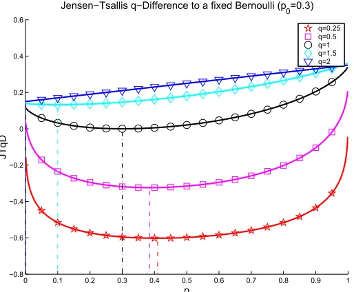
distribution if q_∈[0,1), and closer to a degenerate distribution for q_∈(1,2](see Fig. 1). This is not so surprising: recall that T2(p1,p2) = 1₂−1₂hp1,p2i; in this case, (27) becomes a linear program,

and the solution is not p∗₁=p2, but p∗1=δj, where j=arg maxip2i.

(15)

0 0.1 0.2 0.3 0.4 0.5 0.6 0.7 0.8 0.9 1 −0.8

−0.6 −0.4 −0.2 0 0.2 0.4 0.6

p

JT

q

D

Jensen−Tsallis q−Difference to a fixed Bernoulli (p

0=0.3)

q=0.25 q=0.5 q=1 q=1.5 q=2

Figure 1: Jensen-Tsallis q-difference between two Bernoulli distributions, p1 = (0.3,0.7) and

p2= (p,1−p), for several values of the entropic index q. Observe that, for q∈[0,1),

the minimizer of the JT q-difference approaches the uniform distribution(0.5,0.5)as q approaches 0; for q_∈(1,2], this minimizer approaches the degenerate distribution, as

q_→2.

We start with the following corollary of Proposition 8, which establishes the joint convexity of the JT q-difference, for q_∈[0,1]. (Interestingly, this “complements” the joint convexity of the JT divergence (20), for q_∈[1,2], proved by Burbea and Rao 1982.)

Corollary 9 Let

T

and

X

be finite sets with cardinalities m and n, respectively. For q∈[0,1], the JT q-difference is a jointly convex function on M₊1,Sq(

X

). Formally, let_{pt(i)}t∈T, and i=1, . . . ,l, be

a collection of l sets of probability distributions on

X

thus, from Proposition 8, T_qπ is convex if and only if ϕq is convex and−1/ϕ′′q is(2−q)-convex. Sinceϕ′′_q(x) =q xq−2,ϕqis convex for x≥0 and q≥0. To show the(2−q)-convexity of−1/ϕ′′q(x) =

−(1/q)x2−q, for xt≥0, and q∈[0,1], we use a version of the power mean inequality (Steele, 2006),

−

l

∑

i=1

λixi !2−q

≤ −

l

∑

i=1

(λixi)2−q=− l

∑

i=1

λ2−q i x

(16)

thus concluding that−1/ϕ′′

qis in fact(2−q)-convex.

A consequence of Corollary 9 is that, for finite

X

and any q _∈[0,1], the JT q-difference is upper bounded, namely T_qπ(p1, . . . ,pm)≤Sq(π). Indeed, since Tqπis convex and its domain is the Cartesian product of m simplices (a convex polytope), its maximum must occur on a vertex, that is, when each argument pt is a degenerate distribution at xt, denoted δxt. In particular, if|

X

| ≥ |

T

|,

this maximum occurs at a vertex corresponding to disjoint degenerate distributions, that is, such that

xi6=xj if i6= j. At this maximum,

T_qπ(δx1, . . . ,δxm) = Sq m

∑

t=1

πtδxt !

−

m

∑

t=1

πtSq(δxt)

= Sq

m

∑

t=1

πtδxt !

(28)

= Sq(π)

where the equality in (28) results from Sq(δxt) =0. (Notice that this maximum may not be achieved

∑jψ(p1 j, . . . ,pm j), with

ψ(y1, . . . ,ym) = 1

q₋1

"

∑

i

(πi−πqi)yi+

∑

i

πq iy

q

i −

∑

i

πiyi !q#

.

It suffices to consider the second derivative ofψwith respect to y1. Introducing z=∑mi=2πiyi,

∂2_ψ

∂y2₁ = q

h

πq

1y

q−2 1 −π

2

1(π1y1+z)q−2

i

= qπ2₁(π1y1)q−2−(π1y1+z)q−2

. (31)

Sinceπ1y1≤(π1y1+z)≤1, the quantity in (31) is nonnegative for q∈[0,2]and non-positive for

q_≥2.

5.3 Joint and Conditional JT q-Differences and a Chain Rule

This subsection introduces joint and conditional JT q-differences, which will later be used as a contrast measure between stochastic processes. A chain rule is derived that relates conditional and joint JT q-differences.

Definition 12 Let

X

,

),

• for each y_∈

Y

, the conditionals r(X_|Y =y)_∈M1₊(

X

).

For notational convenience, we also append a subscript to p to emphasize its joint or conditional

de-pendency of the random variables X and Y , that is, pXY ,p, and pX_|Ydenotes a random conditional

probability distribution taking values in{pt(.|Y)}t∈T according to the distributionπ.

For q_≥0, we refer to the joint JT q-difference of pXY by

T_qπ(pXY),Tqπ(p) =Sq(r)−Eq,T∼π(T)[Sq(pt)]

and to the conditional JT q-difference of pX|Y by

T_qπ(pX_|Y),Eq,Y_∼r(Y)[Sq(r(.|Y =y))]−Eq,T_∼π(T)

Eq,Y_∼pt(Y)[Sq(pt(.|Y=y))]

, (32)

(18)

Note that the joint JT q-difference is just the usual JT q-difference of the joint random variable

X_×Y , which equals (cf. 25)

T_qπ(pXY) = Sq(X,Y)−Sq(X,Y|T) = Iq(X×Y ; T), (33)

and the conditional JT q-difference is simply the usual JT q-difference with all entropies replaced by conditional entropies (conditioned on Y ). Indeed, expression (32) can be rewritten as:

T_qπ(pX|Y) = Sq(X|Y)−Sq(X|T,Y) = Iq(X ; T |Y), (34)

that is, the conditional JT q-difference may also interpreted as a Tsallis mutual information, as in (25), but now conditioned on the random variable Y .

Note also that, for the extensive case q=1, (32) may also be rewritten in terms of the conditional KL divergences,

Jπ(p_X_|_Y)_,T₁π(p_X_|_Y) = E_Y_∼_r₍_Y₎[H(r(._|Y =y))]₋E_T_∼_π₍_T₎E_Y_∼_p_t₍_Y₎[H(pt(.|Y =y))]

= ET_∼π(T)

EY_∼r(Y)[D(pt(.|Y =y)kr(.|Y =y))]

.

Proposition 13 The following chain rule holds:

T_qπ(pXY) =Tqπ(pX|Y) +Tqπ(pY)

Proof Writing the joint/conditional JT q-differences as joint/conditional mutual informations (33– 34) and invoking the chain rule provided by (4), we have that

Iq(X ; T|Y) +Iq(Y ; T) = Sq(X|T,Y)−Sq(X|Y) +Sq(Y|T)−Sq(Y)

= Sq(X,Y|T)−Sq(X,Y),

which is the joint JT q-difference associated with the random variable X_×Y .

Let us now turn our attention to the case where Y =Xk for some k_∈N_{. In the following, the} notation(An)n∈Ndenotes a stationary ergodic process with values on some finite alphabet

A

.

Definition 14 Let

X

and

T

be measure spaces, with

X

finite, and letF= [(Xn)n∈N]T be a family of

stochastic processes (taking values on the alphabet

X

) indexed by

T

. The k-th order JT q-difference

ofF _{is defined, for k}₌₁_{, . . . ,}_{n, as}

T_qjoint_,_k ,π(F₎_,_T_qπ₍_p_Xk)

and the k-th order conditional JT q-difference ofF _{is defined, for k}₌₁_{, . . . ,}_{n, as}

T_qcond_,_k ,π(F₎_,_T_qπ₍_p_X

|Xk),

and, for k=0, as T_qcond_,₀ ,π(F₎_,_Tjoint,π

q,1 (F) =Tqπ(pX).

Proposition 15 The joint and conditional k-th order JT q-differences are related through:

T_qjoint_,_k ,π(F_{) =} k₋1

∑

i=0

T_qcond_,_i ,π(F₎ ₍₃₅₎

(19)

5.4 Asymptotic Analysis in the Extensive Case

We now focus on the extensive case (q=1) for a brief asymptotic analysis of the k-th order joint and conditional JT 1-differences (or conditional Jensen-Shannon divergences) when k goes to infinity.

The conditional Jensen-Shannon divergence was introduced by El-Yaniv et al. (1998) to address the two-sample problem for strings emitted by Markovian sources. Given two strings s and t, the goal is to decide whether they were emitted by the same source or by different sources. Under some fair assumptions, the most likely k-th order Markovian joint source of s and t is governed by a distribution ˆr given by

ˆr=arg min

r λD(pˆskr) + (1−λ)D(pˆtkr). (36)

where D(._k.)are conditional KL divergences, ˆps and ˆpt are the empirical(k−1)-th order condi-tionals associated with s and t, respectively, andλ=_|s_|/(_|s_|+_|t_|)is the length ratio. The solution of the optimization problem is

ˆr(a_|c) = λpˆs(c)

λpˆs(c) + (1−λ)pˆt(c) ˆ

ps(a|c) +

(1₋λ)pˆt(c)

λpˆs(c) + (1−λ)pˆt(c) ˆ

pt(a|c),

where a_∈

A

is a symbol and c_∈

A

k−1_{is a context; this can be rewritten as ˆr}₍_a_,_c_{) =}λ_p_ˆ

s(a,c) +

(1₋λ)pˆt(a,c); that is, the optimum in (36) is a mixture of ˆpsand ˆpt weighted by the string lengths. Notice that, at the minimum, we have

λD(pˆskˆr) + (1−λ)D(pˆtkˆr) =JScond_k ,(λ,1−λ)(pˆs,pˆt).

It is tempting to investigate the asymptotic behavior of the conditional and joint JS divergences when k_→∞; however, unlike other asymptotic information theoretic quantities, like the entropy or cross entropy rates, this behavior fails to characterize the sources s and t. Intuitively, this is justified by the fact that observing more and more symbols drawn from the mixture of the two sources rapidly decreases the uncertainty about which source generated the sample. Indeed, from the asymptotic equipartition property of stationary ergodic sources (Cover and Thomas, 1991), we have that limk→∞1kH(pXk) =limk→∞H(pX|Xk), which implies

lim k→∞JS

cond,π

k = _klim

→∞

1

kJS

joint,π

k ≤ _klim

→∞

1

kH(π) = 0,

where we used the fact that the JS divergence is upper-bounded by the entropy of the mixture

H(π)(see Proposition 10). Since the conditional JS divergence must be non-negative, we therefore conclude that limk→∞JSkcond,π=0, pointwise.

6. Nonextensive Mutual Information Kernels

(20)

those kernels under a new information-theoretic light. After that, we give a brief overview of string kernels, and using the results of Section 5.3, we devise k-th order Jensen-Tsallis kernels between stochastic processes that subsume the well-known p-spectrum kernel of Leslie et al. (2002).

6.1 Positive and Negative Definite Kernels

We start by recalling basic concepts from kernel theory (Sch¨olkopf and Smola, 2002); in the fol-lowing,

X

denotes a nonempty set.

Definition 16 Letϕ:

X

_×

X

_→R_{be a symmetric function, that is, a function satisfying}ϕ₍_y_,_x_{) =}

ϕ(x,y), for all x,y_∈

X

.ϕis called a positive definite (pd) kernel if and only if

n

∑

i=1

n

∑

j=1

cicjϕ(xi,xj)≥0

for all n_∈N_{, x}₁_{, . . . ,}_x_n_∈

X

and c1, . . . ,cn∈R.

Definition 17 Letψ:

X

_×

X

_→R_{be symmetric.} ψ_{is called a negative definite (nd) kernel if and}

only if

n

∑

i=1

n

∑

j=1

cicjψ(xi,xj)≤0

for all n_∈N_{, x}₁_{, . . . ,}_x_n_∈

_X

_{and c}₁_{, . . . ,}_c_n_∈R_{, satisfying the additional constraint c}₁₊_{. . .}₊_c_n₌_0.

In this case, ₋ψ is called conditionally pd; obviously, positive definiteness implies conditional

positive definiteness.

The sets of pd and nd kernels are both closed under pointwise sums/integrations, the former being also closed under pointwise products; moreover, both sets are closed under pointwise con-vergence. While pd kernels “correspond” to inner products via embedding in a Hilbert space, nd kernels that vanish on the diagonal and are positive anywhere else, “correspond” to squared Hilber-tian distances. These facts, and the following propositions and lemmas, are shown in Berg et al. (1984).

_→R₊ _{is a nd kernel if and only if}₍_t₊ψ₎−1 _{is pd for all}

t>0.

(21)

Lemma 22 If f :

X

_→R_{satisfies f} _≥_{0, then, for}α_∈_[₁_,₂_]_{, the function}ψ_α₍_x_,_y_{) =}₋₍_f₍_x₎₊_f₍_y₎₎α

is a nd kernel.

The following definition (Berg et al., 1984) has been used in a machine learning context by Cuturi and Vert (2005).

Definition 23 Let(

X

,_⊕) be a semigroup.2 A functionϕ:

X

q_∈(1,2]: Lemma 22 guarantees that the kernel k(x,y) =₋(x+y)q _{is nd; therefore} ₋ιq _{is a nd} function.

For q=1, we use the fact that,

ϕ1(x) =ϕH(x) =−x ln x=lim q→1

x₋xq

q₋1 =qlim→1ϕq(x),

where the limit is obtained by L’Hˆopital’s rule; since the set of nd functions is closed under limits,

ϕ1(x)is nd.

The following lemma, proved in Berg et al. (1984), will also be needed below.

Lemma 25 The functionζq:R++→R, defined asζq(y) =y−qis pd, for q∈[0,1].

We are now in a position to present the main contribution of this section, which is a family of

weighted Jensen-Tsallis kernels, generalizing the JS-based (and other) kernels in two ways: (i) they

allow using unnormalized measures; equivalently, they allow using different weights for each of the two arguments; (ii) they extend the mutual information feature of the JS kernel to the nonextensive scenario.