Cover Tree Bayesian Reinforcement Learning
Nikolaos Tziortziotis [email protected]
Department of Computer Science and Engineering University of Ioannina
GR-45110, Greece
Christos Dimitrakakis [email protected]
Department of Computer Science and Engineering Chalmers University of Technology
SE-41296, Sweden
Konstantinos Blekas [email protected]
Department of Computer Science and Engineering University of Ioannina
GR-45110, Greece
Editor:Laurent Orseau
Abstract
This paper proposes an online tree-based Bayesian approach for reinforcement learning. For inference, we employ a generalised context tree model. This defines a distribution on multivariate Gaussian piecewise-linear models, which can be updated in closed form. The tree structure itself is constructed using the cover tree method, which remains effi-cient in high dimensional spaces. We combine the model with Thompson sampling and approximate dynamic programming to obtain effective exploration policies in unknown en-vironments. The flexibility and computational simplicity of the model render it suitable for many reinforcement learning problems in continuous state spaces. We demonstrate this in an experimental comparison with a Gaussian process model, a linear model and simple least squares policy iteration.
Keywords: Bayesian inference, non-parametric statistics, reinforcement learning
1. Introduction
In reinforcement learning, an agent must learn how to act in an unknown environment from limited feedback and delayed reinforcement. Efficient learning and planning requires models of the environment that are not only general, but can also be updated online with low computational cost. In addition, probabilistic models allow the use of a number of near-optimal algorithms for decision making under uncertainty. While it is easy to construct such models for small, discrete environments, models for the continuous case have so far been mainly limited to parametric models, which may not have the capacity to represent the environment (such as generalised linear models) and to non-parametric models, which do not scale very well (such as Gaussian processes).
data-dependent partitions. They were initially proposed for the problem ofk-nearest neighbour search, but they are in general a good method to generate fine partitions of a state space, due to their low complexity, and can be applied to any state space, with a suitable choice of metric. In addition, it is possible to create a statistical model using the cover tree as a basis. Due to the tree structure, online inference has low (logarithmic) complexity.
In this paper, we specifically investigate the case of a Euclidean state space. For this, we propose a model generalising the context tree weighting algorithm proposed by Willems et al. (1995), combined with Bayesian multivariate linear models. The overall prior can be interpreted as a distribution on piecewise-linear models. We then compare this model with a Gaussian process model, a single linear model, and the model-free method least-squares policy iteration in two well-known benchmark problems in combination with approximate dynamic programming and show that it consistently outperforms other approaches.
The remainder of the paper is organised as follows. Section 1.1 introduces the setting, Section 1.2 discusses related work and Section 1.3 explains our contribution. The model and algorithm are described in Section 2. Finally, comparative experiments are presented in Section 3 and we conclude with a discussion of the advantages of cover-tree Bayesian reinforcement learning and directions of future work in Section 4.
1.1 Setting
We assume that the agent acts within a fully observable discrete-time Markov decision process (MDP), with a metric state space S, for example S ⊂ Rm. At time t, the agent
observes the current environment state st ∈ S, takes an action at from a discrete set A,
and receives a reward rt ∈ R. The probability over next states is given in terms of a
transition kernel Pµ(S | s, a) , Pµ(st+1 ∈ S | st = s, at = a). The agent selects its
actions using a policy π ∈ Π, which in general defines a conditional distribution Pπ(at |
s1, . . . ,st, a1, . . . , at−1, r1, . . . , rt−1) over the actions, given the history of states and actions.
This reflects the learning process that the agent undergoes, when the MDPµis unknown. The agent’s utility is U , P∞
t=0γtrt, the discounted sum of future rewards, with γ ∈
(0,1) a discount factor such that rewards further into the future are less important than immediate rewards. The goal of the agent is to maximise its expected utility:
max
π∈ΠE π
µU = max π∈ΠE
π µ
∞
X
t=0 γtrt,
where the value of the expectation depends on the agent’s policyπ and the environmentµ. If the environment is known, well-known dynamic programming algorithms can be used to find the optimal policy in the discrete-state case (Puterman, 2005), while many approximate algorithms exist for continuous environments (Bertsekas and Tsitsiklis, 1996). In this case, optimal policies are memoryless and we letΠ1 denote the set of memoryless policies. Then MDP and policy define a Markov chain with kernelPµπ(S |s, a) =P
a∈APµ(S |s, a)π(a|s).
How-ever, this is generally extremely complex, as we must optimise over all history-dependent policies.
More specifically, the main assumption in Bayesian reinforcement learning is that the environment µ lies in a given set of environments M. In addition, the agent must select a subjective prior distribution p(µ) which encodes its belief about which environments are most likely. The Bayes-optimal expected utility for p is:
Up∗ , max
π∈ΠDE π
pU = max π∈ΠD
Z
M
EπµU
dp(µ). (1)
Unlike the knownµcase, the optimal policy may not be memoryless, as our belief changes over time. This makes the optimisation over the policies significantly harder (Duff, 2002), as we have to consider the set of all history-dependent deterministic policies, which we denote by ΠD ⊂ Π. In this paper, we employ the simple, but effective, heuristic of Thompson sampling (Thompson, 1933; Wyatt, 1998; Dearden et al., 1998; Strens, 2000) for finding policies. This strategy is known by various other names, such as probability matching, stochastic dominance, sampling-greedy and posterior sampling. Very recently Osband et al. (2013) showed that it suffers small Bayes-regret relative to the Bayes-optimal policy for finite, discrete MDPs.
The second problem in Bayesian reinforcement learning is the choice of the prior distri-bution. This can be of critical importance for large or complex problems, for two reasons. Firstly, a well-chosen prior can lead to more efficient learning, especially in the finite-sample regime. Secondly, as reinforcement learning involves potentially unbounded interactions, the computational and space complexity of calculating posterior distributions, estimating marginals and performing sampling become extremely important. The choice of priors is the main focus of this paper. In particular, we introduce a prior over piecewise-linear mul-tivariate Gaussian models. This is based on the construction of a context tree model, using a cover tree structure, which defines a conditional distribution on local linear Bayesian multivariate models. Since inference for the model can be done in closed form, the result-ing algorithm is very efficient, in comparison with other non-parametric models such as Gaussian processes. The following section discusses how previous work is related to our model.
1.2 Related Work
One component in our model is thecontext tree. Context trees were introduced by Willems et al. (1995) for sequential prediction (see Begleiter et al., 2004, for an overview). In this model, a distribution of variable order Markov models for binary sequences is constructed, where the tree distribution is defined through context-dependent weights (for probability of a node being part of the tree) and Beta distributions (for predicting the next observation). A recent extension to switching time priors (van Erven et al., 2008) has been proposed by Veness et al. (2012). More related to this paper is an algorithm proposed by Kozat et al. (2007) for prediction. This asymptotically converges to the best univariate piecewise linear model in a class of trees with fixed structure.
et al., 2011; Bellemare et al., 2013; Farias et al., 2010).1 However, tree structures can generally be used to perform Bayesian inference in a number of other domains (Paddock et al., 2003; Meila and Jordan, 2001; Wong and Ma, 2010).
The core of our model is a generalised context tree structure that defines a distribution on multivariate piecewise-linear-Gaussian models. Consequently, a necessary component in our model is a multivariate linear model at each node of the tree. Such models were previously used for Bayesian reinforcement learning in Tziortziotis et al. (2013) and were shown to perform well relatively to least-square policy iteration (LSPI, Lagoudakis and Parr, 2003). Other approaches using linear models include Strehl and Littman (2008), which proves mistake bounds on reinforcement learning algorithms using online linear regression, and Abbeel and Ng (2005) who use separate linear models for each dimension. Another related approach in terms of structure is Brunskill et al. (2009), which partitions the space into
types and estimates a simple additive model for each type.
Linear-Gaussian models are naturally generalised by Gaussian processes (GP). Some ex-amples of GP in reinforcement learning include those of Rasmussen and Kuss (2004), Deisen-roth et al. (2009) and Deisenroth and Rasmussen (2011), which focused on a model-predictive approach, while the work of Engel et al. (2005) employed GPs for expected utility estimation. GPs are computationally demanding, in contrast to our tree-structured prior. Another problem with the cited GP-RL approaches is that they employ the marginal distribution in the dynamic programming step. This heuristic ignores the uncertainty about the model (which is implicitly taken into account in Equations 1, 6). A notable exception to this is the policy gradient approach employed by Ghavamzadeh and Engel (2006) which uses full Bayesian quadrature. Finally, output dimensions are treated independently, which may not make good use of the data. Methods for efficient dependent GPs such as the one introduced by Alvarez et al. (2011) have not yet been applied to reinforcement learning.
For decision making, this paper uses the simple idea of Thompson sampling (Thompson, 1933; Wyatt, 1998; Dearden et al., 1998; Strens, 2000), which has been shown to be near-optimal in certain settings (Kaufmann et al., 2012; Agrawal and Goyal, 2012; Osband et al., 2013). This avoids the computational complexity of building augmented MDP models (Auer et al., 2008; Asmuth et al., 2009; Castro and Precup, 2010; Araya et al., 2012), Monte-Carlo tree search (Veness et al., 2011), sparse sampling (Wang et al., 2005), stochastic branch and bound (Dimitrakakis, 2010b) or creating lower bounds on the Bayes-optimal value function (Poupart et al., 2006; Dimitrakakis, 2011). Thus the approach is reasonable as long as sampling from the model is efficient.
1.3 Our Contribution
Our approach is based upon three ideas. The first idea is to employ a cover tree (Beygelzimer et al., 2006) to create a set of partitions of the state space. This avoids having to prespecify a structure for the tree. The second technical novelty is the introduction of an efficient non-parametric Bayesian conditional density estimator on the cover tree structure. This is a generalised context tree, endowed with a multivariate linear Bayesian model at each node. We use this to estimate the dynamics of the underlying environment. The multivariate
models allow for a sample-efficient estimation by capturing dependencies. Finally, we take a sample from the posterior to obtain a piecewise linear Gaussian model of the dynamics. This can be used to generate policies. In particular, from this, we obtain trajectories of simulated experience, to perform approximate dynamic programming (ADP) in order to select a policy. Although other methods could be used to calculate optimal actions, we leave them for future work.
The main advantage of our approach is its generality and efficiency. The posterior cal-culation and prediction is fully conjugate and can be performed online. At the t-th time step, inference takes O(lnt) time. Sampling from the tree, which need only be done infre-quently, is O(t). These properties are in contrast to other non-parametric approaches for reinforcement learning such as GPs. The most computationally heavy step of our algorithm is ADP. However, once a policy is calculated, the actions to be taken can be calculated in logarithmic time at each step. The specific ADP algorithm used is not integral to our approach and for some problems it might be more efficient to use an online algorithm.
2. Cover Tree Bayesian RL
The main idea of cover tree Bayesian reinforcement learning (CTBRL) is to construct a cover tree from the observations, simultaneously inferring a conditional probability density on the same structure, and to then use sampling to estimate a policy. We use a cover tree due to its efficiency compared with e.g., a fixed sequence of partitions or other dynamic partitioning methods such as KD-trees. The probabilistic model we use can be seen as a distribution over piecewise linear-Gaussian densities, with one local linear model for each set in each partition. Due to the tree structure, the posterior can be computed efficiently online. By taking a sample from the posterior, we acquire a specific piecewise linear Gaussian model. This is then used to find an approximately optimal policy using approximate dynamic programming.
An overview of CTBRL is given in pseudocode in Alg. 1. As presented, the algorithm works in an episodic manner.2 When a new episode k starts at time tk, we calculate a new stationary policy by sampling a tree µk from the current posterior ptk(µ). This tree
corresponds to a piecewise-linear model. We draw a large number of rollout trajectories from µk using an arbitrary exploration policy. Since we have the model, we can use an initial state distribution that covers the space well. These trajectories are used to estimate a near-optimal policyπk using approximate dynamic programming. During the episode, we
take new observations usingπk, while growing the cover tree as necessary and updating the posterior parameters of the tree and the local model in each relevant tree node.
We now explain the algorithm in detail. First, we give an overview of the cover tree structure on which the context tree model is built. Then we show how to perform infer-ence on the context tree, while Section 2.3 describes the multivariate model used in each node of the context tree. The sampling approach and the approximate dynamic method are described in Section 2.4, while the overall complexity of the algorithm is discussed in Section 2.5.
Algorithm 1 CTBRL (Episodic, using Thompson sampling)
1: k= 0, π0 =Unif(A), priorp0 on M. 2: fort= 1, . . . , T do
3: if episode-endthen 4: k:=k+ 1.
5: Sample modelµk ∼pt(µ).
6: Calculate policyπk≈arg maxπEπµkU. 7: end if
8: Observe statest.
9: Take action at∼πk(· |st).
10: Observe next state st+1, rewardrt+1.
11: Add a leaf node to the tree Tat, containing st.
12: Update posterior: pt+1(µ) = pt(µ | st+1,st, at) by updating the parameters of all nodes containing st.
13: end for
2.1 The Cover Tree Structure
Cover trees are a data structure that can be applied to any metric space and are, among other things, an efficient method to perform nearest-neighbour search in high-dimensional spaces (Beygelzimer et al., 2006). In this paper, we use cover trees to automatically con-struct a sequence of partitions of the state space. Section 2.1.1 explains the properties of the constructed cover tree. As the formal construction duplicates nodes, in practice we use a reduced tree where every observed point corresponds to one node in the tree. This is explained in Section 2.1.2. An explanation of how nodes are added to the structure is given in Section 2.1.3.
2.1.1 Cover Tree Properties
To construct a cover tree T on a metric space (Z, ψ) we require a set of points Dt = {z1, . . . ,zt}, with zi ∈ Z, a metric ψ, and a constant ζ > 1. We introduce a mapping
function [·] so that the i-th tree node corresponds to one point z[i] in this set. The nodes
are arranged inlevels, with each point being replicated at nodes in multiple levels, i.e., we may have [i] = [j] for some i6=j. Thus, a point corresponds to multiple nodes in the tree, but to at most one node at any one level. Let Gn denote the set of points corresponding
to the nodes at level n of the tree and C(i) ⊂ Gn−1 the corresponding set of children. If i∈Gnthen the level of iis`(i) =n. The tree has the following properties:
1. Refinement: Gn⊂Gn−1.
2. Siblings separation: i, j∈Gn,ψ(z[i],z[j])> ζn.
3. Parent proximity: If i∈Gn−1 then∃a unique j∈Gn such thatψ(z[i],z[j])≤ζn and i∈C(j).
must be close to its parent. These properties directly give rise to the theoretical guarantees given by the cover tree structure, as well as methods for searching and adding points to the tree, as explained below.
2.1.2 The Reduced Tree
As formally the cover tree duplicates nodes, in practice we use the explicit representa-tion (described in more detail in Section 2 of Beygelzimer et al., 2006). This only stores the top-most tree node icorresponding to a point z[i]. We denote this reduced tree by ˆT. Thedepth d(i) of nodei∈Tˆ is equal to its number of ancestors, with the root node having a depth of 0. Aftert observations, the set of nodes containing a pointz, is:
ˆ
Gt(z), n
i∈Tˆ
z∈Bi o
,
where Bi = z∈ Z ψ(z[i],z)≤ζd(i) is the neighbourhood of i. Then ˆGt(z) forms a
path in the tree, as each node only has one parent, and can be discovered in logarithmic time through theFind-Nearest function (Beygelzimer et al., 2006, Theorem 5). This fact allows us to efficiently search the tree, insert new nodes, and perform inference.
2.1.3 Inserting Nodes in the Cover Tree
The cover tree insertion we use is only a minor adaptation of the Insert algorithm by Beygelzimer et al. (2006). For each actiona∈ A, we create a different reduced tree ˆTa, over
the state space, i.e.,Z =S, and build the tree using the metricψ(s,s0) =ks−s0k1. At each point in time t, we obtain a new observation tuple st, at,st+1. We select the
tree ˆTat corresponding to the action. Then, we traverse the tree, decreasingdand keeping
a set of nodes Qd⊂Gd that are ζd-close to st. We stop wheneverQd contains a node that
would satisfy the parent proximity property if we insert the new point at d−1, while the children of all other nodes inQd would satisfy the sibling separation property. This means that we can now insert the new datum as a child of that node.3 Finally, the next statest+1
is only used during the inference process, explained below.
2.2 Generalised Context Tree Inference
In our model, each node i∈ Tˆ is associated with a particular Bayesian model. The main problem is how to update the individual models and how to combine them. Fortunately, a closed form solution exists due to the tree structure. We use this to define a generalised context tree, which can be used for inference.
As with other tree models (Willems et al., 1995; Ferguson, 1974), our model makes predictions by marginalising over a set of simpler models. Each node in the context tree is called acontext, and each context is associated with a specific local model. At timet, given an observation st=sand an action at=a, we calculate the marginal (predictive) density pt of the next observation:
pt(st+1 |st, at) = X
ct
pt(st+1 |st, ct)pt(ct|st, at),
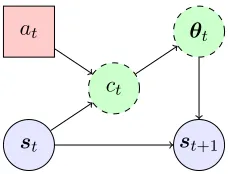
st st+1 at
ct
θt
Figure 1: The generalised context tree graphical model. Blue circles indicate observed vari-ables. Green dashed circles indicate latent varivari-ables. Red rectangles indicate choice variables. Arrows indicate dependencies. Thus, the context distribution at timetdepends on both the state and action, while the parameters depend on the context. The next state depends on the action only indirectly.
where we use the symbolpt throughout for notational simplicity to denote marginal
distri-butions from our posterior at timet. Here,ct is such that ifpt(ct=i|st, at)>0, then the current state is within the neighbourhood of i-th node of the reduced cover tree ˆTat, i.e.,
st∈Bi.
For Euclidean state spaces, the i-th component density pt(st+1 |st, ct = i) employs a
linear Bayesian model, which we describe in the next section. The graphical structure of the model is shown in simplified form in Fig. 1. The context at timetdepends only on the current state st and action at. The context corresponds to a particular local model with
parameterθt, which defines the conditional distribution.
The probability distribution pt(ct |st, at) is determined through stopping probabilities.
More precisely, we set it be equal to the probability of stopping at the i-th context, when performing a walk from the leaf node containing the current observation towards the root, stopping at the j-th node with probability wj,t along the way:
pt(ct=i|st, at) =wi,t Y
j∈Dt(i)
(1−wj,t),
where Dt(i) are the descendants of i that contain the observation st. This forms a path
from i to the leaf node containing st. Note that w0,t = 1, so we always stop whenever
we reach the root. Due to the effectively linear structure of the relevant tree nodes, the stopping probability parameterswcan be updated in closed form, as shown in Dimitrakakis (2010a, Theorem 1) via Bayes’ theorem as follows:
wi,t+1=
pt(st+1 |st, ct=i)wi,t pt(st+1|st, ct∈ {i} ∪Dt(i))
. (2)
Since there is a different tree for each action, ct =i uniquely identifies a tree, the action does not need to enter in the conditional expressions above. Finally, it is easy to see, by marginalisation and the definition of the stopping probabilities, that the denominator in the above equation can be calculated recursively:
Consequently, inference can be performed with a simple forward-backward sweep through a single tree path. In the forward stage, we compute the probabilities of the denominator, until we reach the point where we have to insert a new node. Whenever a new node is inserted in the tree, its weight parameter is initialised to 2−d(i). We then go backwards to the root node, updating the weight parameters and the posterior of each model. The only remaining question is how to calculate the individual predictive marginal distributions for each context i in the forward sweep and how to calculate their posterior in the backward sweep. In this paper, we associate a linear Bayesian model with each context, which provides this distribution.
2.3 The Linear Bayesian Model
In our model we assume that, givenct=i, the next statest+1 is given by a linear
transfor-mation of the current state and additive noise εi,t:
st+1=Aixt+εi,t, xt,
st
1
, (3)
wherext is the current state vector augmented by a unit basis.4 In particular, each context
models the dynamics via a Bayesian multivariate linear-Gaussian model. For the i-th con-text, there is a different (unknown) parameter pair (Ai,Vi) whereAi is the design matrix
and Vi is the covariance matrix. Then the next state distribution is:
st+1|xt=x, ct=i∼N(Aix,Vi).
Thus, the parametersθtwhich are abstractly shown in Fig. 1 correspond to the two matrices A,V. We now define the conditional distribution of these matrices givenct=i.
We can model our uncertainty about these parameters with an appropriate prior dis-tribution p0. In fact, a conjugate prior exists in the form of the matrix inverse-Wishart normal distribution. In particular, givenVi =V, the distribution for Ai is matrix-normal,
while the marginal distribution ofVi is inverse-Wishart:
Ai |Vi =V ∼N(Ai|M,C | {z } prior parameters
,V) (4)
Vi ∼W(Vi| z }| {
W, n). (5)
HereN is the prior on design matrices, which has a matrix-normal distribution, conditional on the covariance and two prior parameters: M, which is the prior mean andC which is the prior covariance of the dependent variable (i.e., the output). Finally,W is the marginal prior on covariance matrices, which has an inverse-Wishart distribution with W and n. More precisely, the distributions have the following forms:
N(Ai|M,C,V)∝e− 1
2tr[(Ai−M)
>V−1(Ai−M)C]
W(V |W, n)∝ |V−1W/2|n/2e−12tr(V
−1W)
.
Essentially, the model extends the classic Bayesian linear regression model (e.g., DeGroot, 1970) to the multivariate case via vectorisation of the mean matrix. Since the prior is conjugate, it is relatively simple to calculate the posterior after each observation. For simplicity, and to limit the total number of prior parameters we have to select, we use the same prior parameters (Mi,Ci,Wi, ni) for all contexts in the tree.
To integrate this with inference in the tree, we must define the marginal distribution used in the nominator of (2). This is a multivariate Student-tdistribution, so if the posterior parameters for contextiat timet are (Mit,Cit,Wit, nti), then this is:
pt(st+1 |xt=x, ct=i) =Student(Mit,Wit/zti,1 +nti),
wherezit= 1−x>(Cit+xx>)−1x.
2.3.1 Regression Illustration
−4 −2 0 2 4
−1 0 1
st
st+1
103 samples
−4 −2 0 2 4
−1 0 1
st 104 samples
E(st+1|st) Ept(st+1|st)
Eµ1ˆ (st+1|st) Eµ2ˆ (st+1|st)
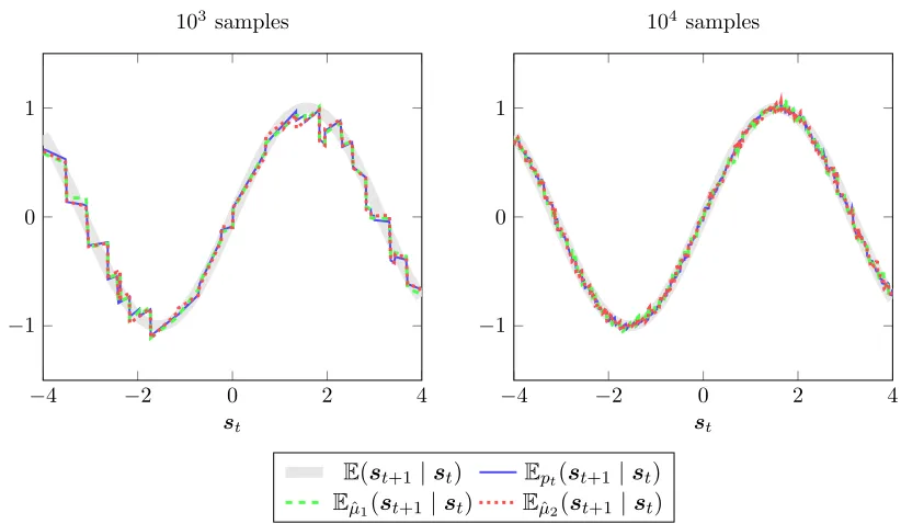
Figure 2: Regression illustration. We plot the expected value for the real distribution, the marginal, as well as two sampled models ˆµ1,µ2ˆ ∼pt(µ).
An illustration of inference using the generalised context tree is given in Fig. 2, where the piecewise-linear structure is evident. The st variates are drawn uniformly in the displayed
interval, while st+1 |st=s ∼N(sin(s),0.1), i.e., drawn a normal distribution with mean
sin(st) and variance 0.1. The plot shows the marginal expectation Ept, as well as the
2.4 Approximating the Optimal Policy with Thompson Sampling
Many algorithms exist for finding the optimal policy for a specific MDPµ, or for calculating the expected utility of a given policy for that MDP. Consequently, a simple idea is to draw MDP samples µi from the current posterior distribution and then calculate the expected
utility of each. This can be used to obtain approximate lower and upper bounds on the Bayes-optimal expected utility by maximising over the set of memoryless policiesΠ1. Taking
K samples, allows us to calculate the upper and lower bounds with accuracyO(1/√K).
max
π∈Π1E π
pU ≈ max π∈Π1
1
K K X
i=1
EπµiU ≤
1 K K X i=1 max
π∈Π1E π
µiU, µi ∼pt(µ). (6)
We consider only the special case K = 1, i.e., when we only sample a single MDP. Then the two values are identical and we recover Thompson sampling. The main problems we have to solve now is how to sample a model and how to calculate a policy for the sampled model.
2.4.1 Sampling a Model from the Posterior
Each model µ sampled from the posterior corresponds to a particular choice of tree pa-rameters. Sampling is done in two steps. The first generates a partition from the tree distribution and the second step generates a linear model for each context in the partition. The first step is straightforward. We only need to sample a set of weights ˆwi ∈ {0,1}
such that P( ˆwi = 1) = wi,t, as shown in Dimitrakakis (2010a, Rem. 2). This creates a partition, with one Bayesian multivariate linear model responsible for each context in the partition.
The second step is to sample a design and covariance matrix pair ( ˆAi,Vˆi) for each
context i in the partition. This avoids sampling matrices for contexts not part of the sampled tree. As the model suggests, we can first sample the noise covariance by plugging the posterior parameters in (5) to obtain ˆVi. Sampling from this distribution can be done
efficiently using the algorithm suggested by Smith and Hocking (1972). We then plug in ˆVi
into the conditional design matrix posterior (4) to obtain a design matrix ˆAi by sampling
from the resulting matrix-normal distribution.
The final MDP sample µfrom the posterior has two elements. Firstly, a set of contexts ˆ
Cµ⊂S
a∈ATˆa, from all action trees. This set is a partition with associated mappingfµ:S × A →Cˆµ. Secondly, a set of associated design and covariance matrices
n
(Aµi, Viµ)
i∈Cˆ
µo
for each context. Then the prediction of the sampled MDP is:
Pµ(st+1|st, at) =N(Aµf(st,at)xt, Vfµ(st,at)), (7)
wherext is given in (3).
2.4.2 Finding a Policy for a Sample via ADP
algorithm, using least-squares temporal differences (LSTD, Bradtke and Barto, 1996) rather than LSTDQ. This is possible because since we haveµavailable, we have access to (7) and it makes LSPI slightly more efficient.
More precisely, consider the value function Vµπ :S →R, defined as:
Vµπ(s),Eµπ(U |st=s).
Unfortunately, for continuousS finding an optimal policy requires approximations. A com-mon approach is to make use of the fact that:
Vµπ(s) =ρ(s) +γ Z
S
Vµπ(s0) dPµπ(s0 |s),
where we assume for simplicity thatρ(s) is the reward obtained at state s. The conditional measure Pµπ is the transition kernel on S induced by µ, π, introduced in Section 1.1. We then select a parametric familyvω :S →Rwith parameter ω∈Ω and minimise:
h(ω) +
Z S
vω(s)−ρ(s)−γ Z
S
vω(s0) d ˆPµπ(s0|s)
dχ(s), (8)
whereh is a regularisation term, χis an appropriate measure on S and ˆPπ
µ is an empirical
estimate of the transition kernel, used to approximate the respective integral that usesPµπ. As we can take an arbitrary number of trajectories fromµ, π, this can be as accurate as our computational capacity allows.
In practice, we minimise (8) with a generalised linear model (defined on an appropriate basis) forvω whileχneed only be positive on a set of representative states. Specifically, we
employ a variant of the least-squares policy iteration (LSPI, Lagoudakis and Parr, 2003) algorithm, using the least-squares temporal differences (LSTD, Bradtke and Barto, 1996) for the minimisation of (8). Then the norm is the euclidean norm and the regularisation term ish(ω) =λkωk. In order to estimate the inner integral, we take KL ≥1 samples from
the model so that
ˆ
Pµπ(s0 |s), 1
KL KL X
i=1
Isit+1=s0 |sit=s , (9)
sit+1|sit=s∼Pµπ(· |s),
where I{·} is an indicator function and Pµπ is decomposable in known terms. Equation
(9) is also used for action selection in order to calculate an approximate expected utility
qω(s, a) for each state-action pair (s, a):
qω(s, a),ρ(s) +γ Z
S
vω(s0) d ˆPµπ(s
0|s)
Effectively, this approximates the integral via sampling. This may add a small amount5 of additional stochasticity to action selection, which can be reduced6 by increasingKL.
Finally, we optimise the policy by approximate policy iteration. At thej-th iteration we obtain an improved policy ˆπj(a |s) ∝P[a∈ arg maxa0∈Aqωj−
1(s, a
0)] from ω
j−1 and then
estimate ωj for the new policy.
5. Generally, this error is bounded byO(KL−1/2).
2.5 Complexity
We now analyse the computational complexity of our approach, including the online com-plexity of inference and decision making, and of the sampling and ADP taking place every episode. It is worthwhile to note two facts. Firstly, that the complexity bounds related to the cover tree depend on a constant c, which however depends on the distribution of samples in the state space. In the worst case (i.e., a uniform distribution), this is bounded exponentially in the dimensionality of the actual state space. While we do not expect this to be the case in practice, it is easy to construct a counterexample where this is the case. Secondly, that the complexity of the ADP step is largely independent of the model used, and mostly depends on the number of trajectories we take in the sampled model and the dimensionality of the feature space.
First, we examine the total computation time that is required to construct the tree.
Corollary 1 Cover tree construction from t observations takes O(tlnt) operations.
Proof In the cover tree, node insertion and query are O(lnt)(Beygelzimer et al., 2006, Theorems 5, 6). Then note that Ptk=1lnk≤Ptk=1lnt=tlnt.
At every step of the process, we must update our posterior parameters. Fortunately, this also takes logarithmic time as we only need to perform calculations for a single path from the root to a leaf node.
Lemma 2 If S ⊂Rm, then inference at time step t has complexityO(m3lnt).
Proof At every step, we must perform inference on a number of nodes equal to the length of the path containing the current observation. This is bounded by the depth of the tree, which is in turn bounded by O(lnt) from Beygelzimer et al. (2006, Lemma 4.3). Calculating (2) is linear in the depth. For each node, however, we must update the linear-Bayesian model, and calculate the marginal distribution. Each requires inverting an m×m matrix, which has complexityO(m3).
Finally, at every step we must choose an action through value function look-up. This again takes logarithmic time, but there is a scaling depending on the complexity of the value function representation.
Lemma 3 If the LSTD basis has dimensionality mL, then taking a decision at time t has complexityO(KLmLlnt).
Proof To take a decision we merely need to search in each action tree to find a corre-sponding path. This takesO(lnt) time for each tree. After Thompson sampling, there will only be one linear model for each action tree. LSTD takes KLoperations, and requires the inner product of two mL-dimensional vectors.
The above lemmas give the following result:
Theorem 4 At time t, the online complexity of CTBRL isO((m3+KLmL) lnt).
Lemma 5 Thompson sampling at time t isO(tm3).
Proof In the worst case, our sampled tree will contain all the leaf nodes of the reduced tree, which areO(t). For each sampled node, the most complex operation is Wishart generation, which isO(m3) (Smith and Hocking, 1972).
Lemma 6 If we use ns samples for LSTD estimation and the basis dimensionality is mL, this step has complexity O(m3L+ns(m2L+KLmLlnt)).
Proof For each sample we must take a decision according to the last policy, which requires
O(KLmLlnt) as shown previously. We also need to update two matrices (see Boyan, 2002),
which isO(m2L). So,O(ns(m2L+KLmLlnt)) computations must be performed for the total number of the selected samples. Since LSTD requires an mL×mL matrix inversion, with complexityO(m3L), we obtain the final result.
From Lemmas 3 and 6 it follows that:
Theorem 7 If we employ API withKAiterations, the total complexity of calculating a new policy is O(tm3+KA(m3L+ns(m2L+KLmLlnt))).
Thus, while the online complexity of CTBRL is only logarithmic in t, there is a sub-stantial cost when calculating a new policy. This is only partially due to the complexity of sampling a model, which is manageable when the state space has small dimensionality. Most of the computational effort is taken by the API procedure, at least as long ast <(mL/m)3. However, we think this is unavoidable no matter what the model used is.
The complexity of Gaussian process (GP) models is substantially higher. In the simplest model, where each output dimension is modelled independently, inference is O(mt3), while the fully multivariate tree model has complexity O(m3tlnt). Since there is no closed form method for sampling a function from the process, one must resort to iterative sampling of points. For n points, the cost is approximately O(nmt3), which makes sampling long trajectories prohibitive. For that reason, in our experiments we only use the mean of the GP.
3. Experiments
We conducted two sets of experiments to analyse the offline and the online performance. We compared CTBRL with the well-known LSPI algorithm (Lagoudakis and Parr, 2003) for the offline case, as well as an online variant (Bu¸soniu et al., 2010) for the online case. We also compared CTBRL with linear Bayesian reinforcement learning (LBRL, Tziortziotis et al., 2013) and finally GP-RL, where we simply replaced the tree model with a Gaussian process. For CTBRL and LBRL we use Thompson sampling. However, since Thompson sampling cannot be performed on GP models, we use the mean GP instead. In order to compute policies given a model, all model-based methods use the variant of LSPI explained in Section 2.4.2. Hence, the only significant difference between each approach is the model used, and whether or not they employ Thompson sampling.
the GP model computationally practical, the greedy approximation approach introduced by Engel et al. (2002) has been adopted. This is a kernel sparsification methodology which incrementally constructs a dictionary of the most representative states. More specifically, anapproximate linear dependence analysis is performed in order to examine whether a state can be approximated sufficiently as a linear combination of current dictionary members or not.
We used one preliminary run and guidance from the literature to make an initial selection of possible hyper-parameters, such as the number of samples and the features used for LSTD and LSTD-Q. We subsequently used 10 runs to select a single hyper-parameter combination for each algorithm-domain pair. The final evaluation was done over an independent set of 100 runs.
For CTBRL and the GP model, we had the liberty to draw an arbitrary number of trajectories for the value function estimation. We drew 1-step transitions from a set of 3000 uniformly drawn states from thesampled model (the mean model in the GP case). We used 25 API iterations on this data.
For the offline performance evaluation, we first drew rollouts from k= {10,20, . . . ,50,
100, . . . ,1000}states drawn from thetrue environment’s starting distribution, using a uni-formly random policy. The maximum horizon of each rollout was set equal to 40. The collected data was then fed to each algorithm in order to produce a policy. This policy was evaluated over 1000 rollouts on the environment.
In the online case, we simply use the last policy calculated by each algorithm at the end of the last episode, so there is no separate learning and evaluation phase. This means that efficient exploration must be performed. For CTBRL, this is done using Thompson sampling. For online-LSPI, we followed the approach of Bu¸soniu et al. (2010), who adopts an -greedy exploration scheme with an exponentially decaying schedule t = td, with 0 = 1. In preliminary experiments, we found d = 0.997 to be a reasonable compromise. We compared the algorithms online for 1000 episodes.
3.1 Domains
We consider two well-known continuous state, discrete-action, episodic domains. The first is the inverted pendulum domain and the second is the mountain car domain.
3.1.1 Inverted Pendulum
sugges-tions of Lagoudakis and Parr (2003). This was replicated for each action for the LSTD-Q
algorithm used in LSPI.
3.1.2 Mountain Car
The aim in this domain is to drive an underpowered car to the top of a hill. Two continuous variables characterise the vehicle state in the domain, its position and its velocity. The objective is to drive an underpowered vehicle up a steep valley from a randomly selected position to the right hilltop (at position>0.5) within 1000 steps. There are three actions: forward, reverse and zero throttle. The received reward is −1 except in the case where the target is reached (zero reward). At the beginning of each rollout, the vehicle is positioned to a new state, with the position and the velocity uniformly randomly selected. The discount factor is set to γ = 0.999. An equidistant 4×4 grid of RBFs over the state space plus a constant term is selected for LSTD and LSPI.
3.2 Results
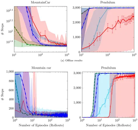
In our results, we show the average performance in terms of number of steps of each method, averaged over 100 runs. For each average, we also plot the 95% confidence interval for the accuracy of the mean estimate with error bars. In addition, we show the 90% percentile region of the runs, in order to indicate inter-run variability in performance.
Figure 3(a) shows the results of the experiments in the offline case. For themountain car, it is clear that CTBRL is significantly more stable compared to GPRL and LSPI. In contrast to the other two approaches, CTBRL needs only a small number of rollouts in order to discover the optimal policy. For the pendulum domain, the performance of both CTBRL and GPRL is almost perfect, as they need only about twenty rollouts in order to discover the optimal policy. On the other hand, LSPI despite the fact that manages to find the optimal policy frequently, around 5% of its runs fail.
Figure 3(b) shows the results of the experiments in the online case. For themountain car, CTBRL managed to find an excellent policy in the vast majority of runs, while con-verging earlier than GPRL and LSPI. Moreover, CTBRL presents a more stable behaviour in contrast to the other two. In the pendulum domain, the performance difference relative to LSPI is even more impressive. It becomes apparent that both CTBRL and GPRL reach near optimal performances with an order of magnitude fewer episodes than LSPI, while the latter remains unstable. In this experiment, we see that CTBRL reaches an optimal policy slightly before GPRL. Although the difference is small, it is very consistent.
101 102 103 101.8
102 102.2 102.4
#
Steps
MountainCar
101 102 103
0 1,000 2,000 3,000
Pendulum
(a) Offline results
100 101 102 103
0 200 400 600 800 1,000
Number of Episodes (Rollouts)
#
Steps
Mountain car
100 101 102 103
0 1,000 2,000 3,000
Number of Episodes (Rollouts) Pendulum
(b) Online results
CTBRL LBRL LSPI GPRL
4. Conclusion
We proposed a computationally efficient, fully Bayesian approach for the exact inference of unknown dynamics in continuous state spaces. The total computation for inference aftertsteps isO(tlnt), in stark contrast to other non-parametric models such as Gaussian processes, which scaleO(t3). In addition, inference is naturally performed online, with the computational cost at timet beingO(lnt).
In practice, the computational complexity is orders of magnitude lower for cover trees than GP, even for these problems. We had to use a dictionary and a lot of tuning to make GP methods work, while cover trees worked out of the box. Another disadvantage of GP methods is that it is infeasible to implement Thompson sampling with them. This is because it is not possible to directly sample a function from the GP posterior. Although Thompson sampling confers no advantage in the offline experiments (as the data there were the same for all methods), we still see that the performance of CTBRL is significantly better on average and that it is much more stable.
Experimentally, we showed that cover trees are more efficient both in terms of compu-tation and in terms of reward, relative to GP models that used the same ADP method to optimise the policy and to a linear Bayesian model which used both the same ADP method and the same exploration strategy. We can see that overall the linear model performs sig-nificantly worse than both GP-RL and CTBRL, though better than -greedy LSPI. This shows that the main reason for the success of CTBRL is the cover tree inference and not the linear model itself, or Thompson sampling.
CTBRL is particularly good in online settings, where the exact inference, combined with the efficient exploration provided by Thompson sampling give it an additional advantage. We thus believe that CTBRL is a method that is well-suited for exploration in unknown continuous state problems. Unfortunately, it is not possible to implement Thompson sam-pling in practice using GPs, as there is no reasonable way to sample a function from the GP posterior. Nevertheless, we found that in both online and offline experiments (where Thompson sampling should be at a disadvantage) the cover tree method achieved superior performance to Gaussian processes.
Although we have demonstrated the method in low dimensional problems, higher di-mensions are not a problem for the cover tree inference itself. The bottleneck is the value function estimation and ADP. This is independent of the model used, however. For example, GP methods for estimating the value function (c.f. Deisenroth et al., 2009) typically have a large number of hyper-parameters for value function estimation, such as choice of represen-tative states and trajectories, kernel parameters and method for updating the dictionary, to avoid problems with many observations.
While in practice ADP can be performed in the background while inference is taking place, and although we seed the ADP with the previous solution, one would ideally like to use a more incremental approach for that purpose. One interesting idea would be to employ a gradient approach in a similar vein to Deisenroth and Rasmussen (2011). An alternative approach would be to employ an online method, in order to avoid estimating a policy for the complete space.7 Promising such approaches include running bandit-based tree search
methods such as UCT (Kocsis and Szepesv´ari, 2006) on the sampled models.
Another direction of future work is to consider more sophisticated exploration policies, particularly for larger problems. Due to the efficiency of the model, it should be possible to compute near-Bayes-optimal policies by applying the tree search method used by Veness et al. (2011). Finally, it would be interesting to examine continuous actions. These can be handled efficiently both by the cover tree and the local linear models by making the next state directly dependent on the action through an augmented linear model. While optimising over a continuous action space is challenging, more recent efficient tree search methods such as metric bandits (Bubeck et al., 2011) may alleviate that problem.
An interesting theoretical direction would be to obtain regret bounds for the problem. This could perhaps be done building upon the analyses of Kozat et al. (2007) for context tree prediction, and of Ortner and Ryabko (2012) for continuous MDPs. The statistical efficiency of the method could be improved by considering edge-based (rather than node-based) distributions on trees, as was suggested by Pereira and Singer (1999).
Finally, as the cover tree method only requires specifying an appropriate metric, the method could be applicable to many other problems. This includes both large discrete problems, and partially observable problems. It would be interesting to see if the approach also gives good results in those cases.
Acknowledgements
We would like to thank the anonymous reviewers, for their careful and detailed comments and suggestions, for this and previous versions of the paper, which have significantly im-proved the manuscript. We also want to thank Mikael K˚ageb¨ack for additional proofreading. This work was partially supported by the Marie Curie Project ESDEMUU “Efficient Se-quential Decision Making Under Uncertainty” , Grant Number 237816 and by an ERASMUS exchange grant.
References
P. Abbeel and A. Y. Ng. Exploration and apprenticeship learning in reinforcement learning. In International Conference on Machine learning (ICML), pages 1–8, 2005.
S. Agrawal and N. Goyal. Analysis of Thompson sampling for the multi-armed bandit problem. In Conference on Learning Theory (COLT), pages 39.1–39.26, 2012.
M. Alvarez, D. Luengo-Garcia, M. Titsias, and N. Lawrence. Efficient multioutput Gaussian processes through variational inducing kernels. InInternational Conference on Artificial Intelligence and Statistics (AISTATS), pages 25–32, 2011.
M. Araya, V. Thomas, and O. Buffet. Near-optimal BRL using optimistic local transitions. In International Conference on Machine Learning (ICML), pages 97–104, 2012.
J. Asmuth, L. Li, M. L. Littman, A. Nouri, and D. Wingate. A Bayesian sampling approach to exploration in reinforcement learning. In Conference on Uncertainty in Artificial In-telligence (UAI), pages 19–26, 2009.
R. Begleiter, R. El-Yaniv, and G. Yona. On prediction using variable order Markov models.
Journal of Artificial Intelligence Research, 22:385–421, 2004.
M. Bellemare, J. Veness, and M. Bowling. Bayesian learning of recursively factored envi-ronments. In International Conference on Machine Learning (ICML), pages 1211–1219, 2013.
D. P. Bertsekas and J. N. Tsitsiklis. Neuro-Dynamic Programming. Athena Scientific, 1996.
A. Beygelzimer, S. Kakade, and J. Langford. Cover trees for nearest neighbor. In Interna-tional Conference on Machine Learning (ICML), pages 97–104, 2006.
J. A. Boyan. Technical update: Least-squares temporal difference learning. Machine Learn-ing, 49(2):233–246, 2002.
S. J. Bradtke and A. G. Barto. Linear least-squares algorithms for temporal difference learning. Machine Learning, 22(1):33–57, 1996.
E. Brunskill, B. R. Leffler, L. Li, M. L. Littman, and N. Roy. Provably efficient learning with type parametric models. Journal of Machine Learning Research, 10:1955–1988, 2009.
S. Bubeck, R. Munos, G. Stoltz, and C. Szepesv´ari. X-armed bandits. Journal of Machine Learning Research, 12:1655–1695, 2011.
L. Bu¸soniu, D. Ernst, B. De Schutter, and R. Babuˇska. Online least-squares policy iteration for reinforcement learning control. In American Control Conference (ACC), pages 486– 491, 2010.
P. Castro and D. Precup. Smarter sampling in model-based Bayesian reinforcement learning.
Machine Learning and Knowledge Discovery in Databases, pages 200–214, 2010.
M. Daswani, P. Sunehag, and M. Hutter. Feature reinforcement learning using looping suffix trees. In European Workshop on Reinforcement Learning (EWRL), pages 11–24, 2012.
R. Dearden, N. Friedman, and S. J. Russell. Bayesian Q-learning. In AAAI/IAAI, pages 761–768, 1998. URL citeseer.ist.psu.edu/dearden98bayesian.html.
M. H. DeGroot. Optimal Statistical Decisions. John Wiley & Sons, 1970.
M. P. Deisenroth and C. E. Rasmussen. PILCO: A model-based and data-efficient approach to policy search. In International Conference on Machine Learning (ICML), pages 465– 472, 2011.
M. P. Deisenroth, C. E. Rasmussen, and J. Peters. Gaussian process dynamic programming.
Neurocomputing, 72(7-9):1508–1524, 2009.
C. Dimitrakakis. Complexity of stochastic branch and bound methods for belief tree search in Bayesian reinforcement learning. In International Conference on Agents and Artificial Intelligence (ICAART), pages 259–264, 2010b.
C. Dimitrakakis. Robust bayesian reinforcement learning through tight lower bounds. In
European Workshop on Reinforcement Learning (EWRL), pages 177–188, 2011.
C. Dimitrakakis, N. Tziortziotis, and A. Tossou. Beliefbox: A framework for statistical methods in sequential decision making. http://code.google.com/p/beliefbox/, 2007.
M. Duff. Optimal Learning Computational Procedures for Bayes-adaptive Markov Decision Processes. PhD thesis, University of Massachusetts at Amherst, 2002.
Y. Engel, S. Mannor, and R. Meir. Sparse online greedy support vector regression. In
European Conference on Machine Learning (ECML), pages 84–96, 2002.
Y. Engel, S. Mannor, and R. Meir. Reinforcement learning with Gaussian process. In
International Conference on Machine Learning (ICML), pages 201–208, 2005.
D. Ernst, P. Geurts, and L. Wehenkel. Tree-based batch mode reinforcement learning.
Journal of Machine Learning Research, 6:503–556, 2005.
V. F. Farias, C. C. Moallemi, B. Van Roy, and T. Weissman. Universal reinforcement learning. IEEE Transactions on Information Theory, 56(5):2441–2454, 2010.
T. S. Ferguson. Prior distributions on spaces of probability measures. The Annals of Statistics, 2(4):615–629, 1974.
M. Ghavamzadeh and Y. Engel. Bayesian policy gradient algorithms. InAdvances in Neural Information Processing Systems (NIPS), pages 457–464, 2006.
E. Kaufmann, N. Korda, and R. Munos. Thompson sampling: An optimal finite time analysis. In Algorithmic Learning Theory (ALT), pages 199–213, 2012.
L. Kocsis and C. Szepesv´ari. Bandit based Monte-Carlo planning. InEuropean Conference on Machine Learning (ECML), pages 282–293, 2006.
S. S. Kozat, A. C. Singer, and G. C. Zeitler. Universal piecewise linear prediction via context trees. IEEE Transactions on Signal Processing, 55(7):3730–3745, 2007.
M. G. Lagoudakis and R. Parr. Least-squares policy iteration. The Journal of Machine Learning Research, 4:1107–1149, 2003.
M. Meila and M. I. Jordan. Learning with mixtures of trees. The Journal of Machine Learning Research, 1:1–48, 2001.
I. Osband, D. Russo, and B. Van Roy. (More) efficient reinforcement learning via posterior sampling. In Advances in Neural Information Processing Systems (NIPS), pages 3003– 3011, 2013.
S. M. Paddock, F. Ruggeri, M. Lavine, and M. West. Randomized Polya tree models for nonparametric Bayesian inference. Statistica Sinica, 13(2):443–460, 2003.
F. C. Pereira and Y. Singer. An efficient extension to mixture techniques for prediction and decision trees. Machine Learning, 36(3):183–199, 1999.
P. Poupart, N. Vlassis, J. Hoey, and K. Regan. An analytic solution to discrete Bayesian reinforcement learning. InInternational Conference on Machine Learning (ICML), pages 697–704, 2006.
M. L. Puterman. Markov Decision Processes : Discrete Stochastic Dynamic Programming. John Wiley & Sons, New Jersey, US, 2005.
C. E. Rasmussen and M. Kuss. Gaussian processes in reinforcement learning. InAdvances in Neural Information Processing Systems (NIPS), pages 751–759, 2004.
W. B. Smith and R. R. Hocking. Wishart variates generator, algorithm AS 53. Applied Statistics, 21:341–345, 1972.
A. L. Strehl and M. L. Littman. Online linear regression and its application to model-based reinforcement learning. In Advances in Neural Information Processing Systems (NIPS), pages 1417–1424, 2008.
M. Strens. A Bayesian framework for reinforcement learning. In International Conference on Machine Learning (ICML), pages 943–950, 2000.
W. R. Thompson. On the likelihood that one unknown probability exceeds another in view of the evidence of two samples. Biometrika, 25(3-4):285–294, 1933.
N. Tziortziotis, C. Dimitrakakis, and K. Blekas. Linear Bayesian reinforcement learning. In
International Joint Conference on Artificial Intelligence (IJCAI), pages 1721–1728, 2013.
T. van Erven, P. D. Gr¨unwald, and S. de Rooij. Catching up faster by switching sooner: a prequential solution to the AIC-BIC dilemma. arXiv, 2008. A preliminary version appeared in NIPS 2007.
J. Veness, K. S. Ng, M. Hutter, W. Uther, and D. Silver. A Monte-Carlo AIXI approxima-tion. Journal of Artificial Intelligence Research, 40:95–142, 2011.
J. Veness, K. S. Ng, M. Hutter, and M. Bowling. Context tree switching. In Data Com-pression Conference (DCC), pages 327–336, 2012.
F. M. J. Willems, Y. M. Shtarkov, and T. J. Tjalkens. The context tree weighting method: basic properties. IEEE Transactions on Information Theory, 41(3):653–664, 1995.
W. H. Wong and L. Ma. Optional P´olya tree and Bayesian inference. The Annals of Statistics, 38(3):1433–1459, 2010.