Truncated Power Method for Sparse Eigenvalue Problems
Xiao-Tong Yuan [email protected]
Tong Zhang [email protected]
Department of Statistics Rutgers University New Jersey, 08816, USA
Editor:Hui Zou
Abstract
This paper considers the sparse eigenvalue problem, which is to extract dominant (largest) sparse eigenvectors with at mostknon-zero components. We propose a simple yet effective solution called truncated power methodthat can approximately solve the underlying nonconvex optimization prob-lem. A strong sparse recovery result is proved for the truncated power method, and this theory is our key motivation for developing the new algorithm. The proposed method is tested on applica-tions such as sparse principal component analysis and the densestk-subgraph problem. Extensive experiments on several synthetic and real-world data sets demonstrate the competitive empirical performance of our method.
Keywords: sparse eigenvalue, power method, sparse principal component analysis, densestk-subgraph
1. Introduction
Given a p×psymmetric positive semidefinite matrixA, thelargest k-sparse eigenvalueproblem aims to maximize the quadratic formx⊤Ax with a sparse unit vectorx∈Rpwith no more thank
non-zero elements:
λmax(A,k) =max
x∈Rpx
⊤Ax, subject tokxk=1, kxk
0≤k, (1)
wherek · k denotes theℓ2-norm, and k · k0 denotes theℓ0-norm which counts the number of non-zero entries in a vector. The sparsity is controlled by the values of k and can be viewed as a design parameter. In machine learning applications, for example, principal component analysis, this problem is motivated from the following perturbation formulation of matrixA:
A=A¯+E, (2)
where A is the empirical covariance matrix, ¯A is the true covariance matrix, and E is a random perturbation due to having only a finite number of empirical samples. If we assume that the largest eigenvector ¯xof ¯A is sparse, then a natural question is to recover ¯xfrom the noisy observation A
when the errorE is “small”. In this context, the problem (1) is also referred to as sparse principal component analysis (sparse PCA).
known to be NP-hard. Various researchers have proposed approximate optimization methods: some are based on greedy procedures (e.g., Moghaddam et al., 2006; Jolliffe et al., 2003; d’Aspremont et al., 2008), and some others are based on various types of convex relaxation or reformulation (e.g., d’Aspremont et al., 2007; Zou et al., 2006; Journ´ee et al., 2010). Statistical analysis of sparse PCA has also received significant attention. Under the high dimensional single spike model, John-stone (2001) proved the consistency of PCA using a subset of features corresponding to the largest sample variances. Under the same single spike model, Amini and Wainwright (2009) established conditions for recovering the non-zero entries of eigenvectors using the convex relaxation method of d’Aspremont et al. (2007). However, these results were concerned with variable selection con-sistency under a relatively simple and specific example with limited general applicability. More recently, Paul and Johnstone (2012) studied an extension called multiple spike model, and proposed an augmented sparse PCA method for estimating each of the leading eigenvectors and investigated the rate of convergence of their procedure in the high dimensional setting. In another recent work that is independent of ours, Ma (2013) analyzed an iterative thresholding method for recovering the sparse principal subspace. Although it also focused on the multiple spike covariance model, the pro-cedures and techniques considered there are closely related to the method studied in this paper. In addition, Shen et al. (2013) analyzed the consistency of the sparse PCA method of Shen and Huang (2008), and Cai et al. (2012) analyzed the optimal convergence rate of sparse PCA and introduced an adaptive procedure for estimating the principal subspace.
This paper proposes and analyzes a computational procedure calledtruncated power iteration
methodthat approximately solves (1). This method is similar to the classical power method, with
an additional truncation operation to ensure sparsity. We show that if the true matrix ¯Ahas a sparse (or approximately sparse) dominant eigenvector ¯x, then under appropriate assumptions, this algo-rithm can recover ¯xwhen the spectral norm of sparse submatrices of the perturbation E is small. Moreover, this result can be proved under relative generality without restricting ourselves to the rather specific spike covariance model. Therefore our analysis provides strong theoretical support for this new method, and this differentiates our proposal from previous studies. We have applied the proposed method to sparse PCA and to the densestk-subgraph finding problem (with proper modi-fication). Extensive experiments on synthetic and real-world large-scale data sets demonstrate both the competitive sparse recovering performance and the computational efficiency of our method.
It is worth mentioning that the truncated power method developed in this paper can also be applied to thesmallest k-sparse eigenvalueproblem given by:
λmin(A,k) =min
x∈Rp x
⊤Ax, subject tokxk=1, kxk0≤k, which also has many applications in machine learning.
1.1 Notation
Let Sp ={A∈Rp×p |A=A⊤} denote the set of symmetric matrices, and S+p ={A∈Sp,A
0} denote the cone of symmetric, positive semidefinite matrices. For any A∈Sp, we denote its
eigenvalues byλmin(A) =λp(A)≤ ··· ≤λ1(A) =λmax(A). We useρ(A)to denote the spectral norm ofA, which is max{|λmin(A)|,|λmax(A)|}, and define
ρ(A,s):=max{|λmin(A,s)|,|λmax(A,s)|}. (3)
Thei-th entry of vectorxis denoted by[x]iwhile[A]i j denotes the element on thei-th row and j-th
submatrix ofAwith rows and columns indexed in setF. If necessary, we also denoteAF as the
restriction ofAon the rows and columns indexed inF. Letkxkp be theℓp-norm of a vectorx. In
particular, kxk2=√x⊤x denotes the Euclidean norm,kxk1=∑d
i=1|[x]i|denotes theℓ1-norm, and kxk0=#{j:[x]j6=0}denotes theℓ0-norm. For simplicity, we also denote theℓ2normkxk2bykxk. In the rest of the paper, we defineQ(x):=x⊤Ax. We let supp(x):={j:[x]j6=0}denote the support
set of vectorx. Given an index setF, we define
x(F):=arg max
x∈Rp
x⊤Ax, subject tokxk=1, supp(x)⊆F.
Finally, we denote byIp×pthep×pidentity matrix.
1.2 Paper Organization
The remaining of this paper is organized as follows: §2 describes the truncated power iteration algo-rithm that approximately solves problem (1). In §3 we analyze the solution quality of the proposed algorithm. §4 evaluates the relevance of our theoretical prediction and the practical performance of the proposed algorithm in applications of sparse PCA and the densestk-subgraph finding problems. We conclude this work and discuss potential extensions in §5.
2. Truncated Power Method
Since λmax(A,k) equals λmax(A∗k) whereA∗k is thek×k principal submatrix of A with the largest
eigenvalue, one may solve (1) by exhaustively enumerating all subsets of {1, . . . ,p}of size k in order to findA∗k. However, this procedure is impractical even for moderate sizedksince the number of subsets is exponential ink.
2.1 Algorithm
Therefore in order to solve the spare eigenvalue problem (1) more efficiently, we consider an itera-tive procedure based on the standard power method for eigenvalue problems, while maintaining the desired sparsity for the intermediate solutions. The procedure, presented in Algorithm 1, generates a sequence of intermediatek-sparse eigenvectorsx0,x1, . . .from an initial sparse approximationx0. At each time stampt, the intermediate vectorxt−1is multiplied byA, and then the entries are trun-cated to zeros except for the largestkentries. The resulting vector is then normalized to unit length, which becomesxt. The cardinalitykis a free parameter in the algorithm. If no prior knowledge
of sparsity is available, then we have to tune this parameter, for example, through cross-validation. Note that our theory does not require choosingkprecisely (see Theorem 4), and thus the tuning is not difficult in practice. At each iteration, the computational complexity is inO(k p+p)which is
O(k p)for matrix-vector productAxt−1andO(p)1for selectingklargest elements from the obtained vector of length pto getFt.
Definition 1 Given a vector x and an index set F, we define the truncation operation Truncate(x,F)
to be the vector obtained by restricting x to F, that is
[Truncate(x,F)]i=
[x]i i∈F
0 otherwise .
Algorithm 1:Truncated Power (TPower) Method
Input : matrixA∈Sp, initial vectorx
0∈Rp
Output :xt
Parameters : cardinalityk∈ {1, ...,p}
Lett=1.
repeat
Computex′t=Axt−1/kAxt−1k.
LetFt=supp(x′t,k)be the indices ofx′t with the largestkabsolute values.
Compute ˆxt=Truncate(xt′,Ft).
Normalizext=xˆt/kxˆtk.
t←t+1.
untilConvergence;
Remark 2 Similar to the behavior of traditional power method, if A∈Sp
+, then TPower tries to
find the (sparse) eigenvector of A corresponding to the largest eigenvalue. Otherwise, it may find the (sparse) eigenvector with the smallest eigenvalue if−λp(A)>λ1(A). However, this situation is
easily detectable because it can only happen whenλp(A)<0. In such case, we may restart TPower
with A replaced by an appropriately shifted version A+˜λIp×p.
2.2 Convergence
We now show that whenAis positive semidefinite, TPower converges. This claim is a direct conse-quence of the following proposition.
Proposition 3 If all 2k×2k principal submatrix A2k of A are positive semidefinite, then the
se-quence{Q(xt)}t≥1is monotonically increasing, where xt is obtained from the TPower algorithm.
Proof Observe that the iteratext in TPower solves the following constrained linear optimization
problem:
xt= arg max
kxk=1,kxk0≤k
L(x;xt−1), L(x;xt−1):=h2Axt−1,x−xt−1i.
Clearly, Q(x)−Q(xt−1) =L(x;xt−1) + (x−xt−1)⊤A(x−xt−1). Sincekxt−xt−1k0≤2k and each 2k×2kprincipal submatrix ofAis positive semidefinite, we have(xt−xt−1)⊤A(xt−xt−1)≥0. It follows thatQ(xt)−Q(xt−1)≥L(xt;xt−1). By the definition ofxt as the maximizer of L(x;xt−1) over x (subject to kxk=1 and kxk0 ≤k), we have L(xt;xt−1)≥L(xt−1;xt−1) = 0. Therefore
Q(xt)−Q(xt−1)≥0, which proves the desired result.
3. Sparse Recovery Analysis
We consider the general noisy matrix model (2), and are especially interested in the high dimen-sional situation where the dimension pofAis large. We assume that the noise matrixE is a dense
norm of the full matrix perturbation errorρ(E)can be large. For example, if the original covariance is corrupted by an additive standard Gaussian iid noise vector, thenρ(E,s) =O(pslogp/n), which grows linearly in√s, instead ofρ(E) =O(p
p/n), which grows linearly in√p. The main advan-tage of the sparse eigenvalue formulation (1) over the standard eigenvalue formulation is that the estimation error of its optimal solution depends onρ(E,s)with respectively a smalls=O(k)rather thanρ(E). This linear dependency on sparsitykinstead of the original dimension pis analogous to similar results for sparse regression (or compressive sensing). In fact, the restricted perturbation error considered here is analogous to the idea of restricted isometry property (RIP) considered by Candes and Tao (2005).
The purpose of the section is to show that if matrix ¯A has a unique sparse (or approximately sparse) dominant eigenvector, then under suitable conditions, TPower can (approximately) recover this eigenvector from the noisy observationA.
Assumption 1 Assume that the largest eigenvalue of A¯ ∈Sp is λ =λ
max(A¯) >0 that is
non-degenerate, with a gap∆λ=λ−maxj>1|λj(A¯)|between the largest and the remaining eigenvalues.
Moreover, assume that the eigenvectorx corresponding to the dominant eigenvalue¯ λis sparse with
cardinalityk¯=kx¯k0.
We want to show that under Assumption 1, if the spectral norm ρ(E,s) of the error matrix is small for an appropriately chosens>k¯, then it is possible to approximately recover ¯x. Note that in the extreme case ofs=p, this result follows directly from the standard eigenvalue perturbation analysis (which does not require Assumption 1).
We now state our main result as below, which shows that under appropriate conditions, the TPower method can recover the sparse eigenvector. The final error bound is a direct generalization of standard matrix perturbation result that depends on the full matrix perturbation errorρ(E). Here this quantity is replaced by the restricted perturbation errorρ(E,s).
Theorem 4 We assume that Assumption 1 holds. Let s=2k+k with k¯ ≥k. Assume that¯ ρ(E,s)≤
∆λ/2. Define
γ(s):=λ−∆λ+ρ(E,s)
λ−ρ(E,s) <1, δ(s):=
√
2ρ(E,s)
p
ρ(E,s)2+ (∆λ−2ρ(E,s))2.
If|x⊤0x¯| ≥θ+δ(s)for somekx0k0≤k,kx0k=1, andθ∈(0,1)such that
µ=
q
(1+2((k¯/k)1/2+k¯/k))(1−0.5θ(1+θ)(1−γ(s)2))<1, (4)
then we either have
q
1− |x⊤0x¯|<√10δ(s)/(1−µ), (5)
or for all t≥0
q
1− |x⊤t x¯| ≤µt
q
1− |x⊤0x¯|+√10δ(s)/(1−µ). (6)
Remark 5 We only state our result with a relatively simple but easy to understand quantityρ(E,s), which we refer to as restricted perturbation error. It is analogous to the RIP concept (Candes and
Tao, 2005), and is also directly comparable to the traditional full matrix perturbation errorρ(E).
Remark 6 Although we state the result by assuming that the dominant eigenvectorx is sparse, the¯
theorem can also be adapted to certain situations thatx is only approximately sparse. In such case,¯
we simply letx¯′be ak sparse approximation of¯ x. If¯ x¯′−x is sufficiently small, then¯ x¯′is the dominant
eigenvector of a symmetric matrixA¯′ that is close toA; hence the theorem can be applied with the¯
decomposition A=A¯′+E′where E′=E+A−A¯′.
Note that we did not make any attempt to optimize the constants in Theorem 4, which are relatively large. Therefore in the discussion, we shall ignore the constants, and focus on the main message Theorem 4 conveys. If ρ(E,s) is smaller than the eigen-gap ∆λ/2>0, then γ(s)<1 andδ(s) =O(ρ(E,s)). It is easy to check that for anyk≥k¯, if γ(s) is sufficiently small then the requirement (4) can be satisfied for a sufficiently smallθof the order(k¯/k)1/2. It follows that under appropriate conditions, as long as we can find an initialx0such that
|x⊤0x¯| ≥c(ρ(E,s) + (k¯/k)1/2) for some constantc, then 1− |x⊤t x¯|converges geometrically until
kxt−x¯k=O(ρ(E,s)).
This result is similar to the standard eigenvector perturbation result stated in Lemma 10 of Ap-pendix A, except that we replace the spectral errorρ(E)of the full matrix by ρ(E,s) that can be significantly smaller when s≪ p. To our knowledge, this is the first sparse recovery result for the sparse eigenvalue problem in a relatively general setting. This theorem can be considered as a strong theoretical justification of the proposed TPower algorithm that distinguishes it from earlier algorithms without theoretical guarantees. Specifically, the replacement of the full matrix perturba-tion errorρ(E)withρ(E,s)gives the theoretical insights on why TPower works well in practice.
To illustrate our result, we briefly describe a consequence of the theorem under the single spike covariance model of Johnstone (2001) which was investigated by Amini and Wainwright (2009). We assume that the observations arepdimensional vectors
xi=x¯+ε,
fori=1, . . . ,n, whereε∼N(0,Ip×p). For simplicity, we assume thatkx¯k=1. The true covariance
is
¯
A=x¯x¯⊤+Ip×p,
andAis the empirical covariance
A=1
n
n
∑
i=1
xix⊤i .
LetE=A−A¯, then random matrix theory implies that with large probability,
ρ(E,s) =O(pslnp/n).
Now assume that maxj|x¯j|is sufficiently large. In this case, we can run TPower with a starting
pointx0=ejfor some vectorej (whereej is the vector of zeros except the j-th entry being one) so
(k¯/k)1/2)is satisfied withs=O(k¯). We may run TPower with an appropriate initial vector to obtain an approximate solutionxt of error
kxt−x¯k=O( q
¯
klnp/n).
This bound is optimal (Cai et al., 2012). Note that our results are not directly comparable to those of Amini and Wainwright (2009), which studied support recovery. Nevertheless, it is worth noting that if maxj|x¯j|is sufficiently large, then our result becomes meaningful whenn=O(k¯lnp); however
their result requiresn=O(k¯2lnp)to be meaningful, although this is for the pessimistic case of ¯x
having equal nonzero values of 1/√k¯. Based on a similar spike covariance model, Ma (2013) inde-pendently presented and analyzed an iterative thresholding method for recovering sparse orthogonal principal components, using ideas related to what we present in this paper.
Finally we note that if we cannot find an initial vector with large enough value |x⊤0x¯|, then it may be necessary to take a relatively largekso that the requirement |x⊤0x¯| ≥c(ρ(E,s) + (k¯/k)1/2) is satisfied. With such ak, ρ(E,s)may be relatively large and hence the theorem indicates thatxt
may not converge to ¯x accurately. Nevertheless, as long as|x⊤t x¯|converges to a value that is not too small (e.g., can be much larger than |x⊤0x¯|), we may reduce k and rerun the algorithm with a
k-sparse truncation ofxt as initial vector together with the reduced k. In this two stage process,
the vector found from the first stage (with large k) is truncated and normalized, and then used as the initial value of the second stage (with small k). Therefore we may also regard it as an initialization method for TPower. Specially, in the first stage we may run TPower withk=pfrom arbitrary initialization. In this stage, TPower reduces to the classic power method which outputs the dominant eigenvectorxofA. LetF=supp(x,k)be the indices ofxwith the largestkabsolute values andx0:=Truncate(x,F)/kTruncate(x,F)k. Letθ=x⊤x¯−(k¯/k)1/2
p
1−(x⊤x¯)2−δ(s). It is implied by Lemma 12 in Appendix A thatx⊤0x¯≥θ+δ(s). Obviously, ifθ(1+θ)≥8(k¯/k)/((1+ 4¯k/k)(1−γ(s)2)), thenx
0will be an initialization suitable for Theorem 1. From this initialization, we can obtain a better solution using the TPower method. In practice, one may use other methods to obtain an approximatex0to initialize TPower, not necessarily restricted to running TPower with largerk.
4. Experiments
In this section, we first show numerical results (in §4.1) that confirm the relevance of our theoretical predictions. We then illustrate the effectiveness of TPower method when applied to sparse principal component analysis (sparse PCA) (in §4.2) and the densestk-subgraph (DkS) finding problem (in §4.3). The Matlab code for reproducing the experimental results reported in this section is available fromhttps://sites.google.com/site/xtyuan1980/publications.
4.1 Simulation Study
with true covariance
¯
A=βx¯x¯⊤+Ip×p
and empirical covariance
A=1
n
n
∑
i=1
xix⊤i ,
wherexi∼
N
(0,A¯). For the true covariance matrix ¯A, its dominant eigenvector is ¯x witheigen-value β+1, and its eigenvalue gap is ∆λ=β. For this model, with large probability we have
ρ(E,s) =O(p
slnp/n). Therefore, for fixed dimensionality p, the error bound is relevant to the triplet {n,β,k}. In this study, we consider a setup with p=1000, and ¯x is a ¯k-sparse uniform random vector with ¯k=20 andkx¯k=1. We are interested in the following two cases:
1. Cardinalitykis tuned and fixed: we will study how the estimation error is affected by sample sizenand eigen-gapβ.
2. Cardinality k is varying: for fixed sample size n and eigen-gap β, we will study how the estimation error is affected by cardinalitykin the algorithm.
4.1.1 ONINITIALIZATION
Theorem 4 suggests that TPower can benefit from a good initial vectorx0. We initializex0by using the warm-start strategy suggested at the end of §3. In our implementation, this strategy is specialized as follows: we sequentially run TPower with cardinality{8k,4k,2k,k}, using the (truncated) output from the previous running as the initial vector for the next running. This initialization strategy works satisfactory in our numerical experiments.
4.1.2 TESTI: CARDINALITYk ISTUNEDANDFIXED
In this case, we test withn∈ {100,200,500,1000,2000}andβ∈ {1,10,50,100,200,400}. For each pair {n,β}, we generate 100 empirical covariance matrices and employ the TPower to compute a
k-sparse eigenvector ˆx. For each empirical covariance matrixA, we also generate an independent empirical covariance matrixAvalto selectkfrom the candidate set
K
={5,10,15, ...,50}bymaxi-mizing the following criterion: ˆ
k=arg max
k∈K
ˆ
x(k)⊤Avalxˆ(k),
where ˆx(k) is the output of TPower forAunder cardinality k. For different pairs(n,β), the tuned values of k could be different. For example, for(n,β) = (100,1),k=10 will be selected; while for(n,β) = (100,10), k=20 will be selected. Note that Theorem 4 does not require an accurate estimation ofk. Figure 1(a) shows the estimation error curves as functions ofβunder variousn. It can be observed that for any fixedn, the estimation error decreases as eigen-gapβincreases; and for any fixedβ, the estimation error decreases as sample sizenincreases. This is consistent with the prediction of Theorem 4.
4.1.3 TESTII: CARDINALITYkISVARYING
0 100 200 300 400 -4
-3 -2 -1 0
Eigen-gap β
Estimation Error
Simulated Data
n = 100 n = 200 n = 500 n = 1000 n = 2000
(a) Estimation errorvs.eigen-gapβ(under various sample sizen).
100 200 300 400 500
-4 -3 -2 -1 0
Cardinality k
Estimation Error
Simulated Data
n = 500, β = 400: experimental error n = 500 β = 400: theoretical bound
(b) Estimation error boundvs.cardinalityk(withn=500 and β=400). Both theoretical and empirical curves are plotted.
Figure 1: Estimation error curves on the simulated data. For better viewing, please see the original pdf file.
curves as functions ofk. It can be observed that the estimation error becomes larger askincreases. This is consistent with the prediction of Theorem 4. For a fixedk, provided that the conditions are satisfied in Theorem 4, we can also calculate the theoretical estimation error bound√10δ(s)/(1−
µ). The curve of the theoretical bound is plotted in the same figure. As predicted by Theorem 4, the theoretical bound curve dominates the empirical error curve. Similar observations are also made for other fixed pairs{n,β}.
4.2 Sparse PCA
learning method for matrix decomposition with sparsity regularization. More recently, Journ´ee et al. (2010) studied a generalized power method to solve sparse PCA with a certain dual reformulation of the problem. Similar power-truncation-type methods were also considered by Witten et al. (2009) and Ma (2013).
Given a sample covariance matrix, Σ∈Sp+ (or equivalently a centered data matrix D∈Rn×p
withn rows of p-dimensional observations vectors such thatΣ=D⊤D) and the target cardinality
k, following the literature (Moghaddam et al., 2006; d’Aspremont et al., 2007, 2008), we formulate sparse PCA as:
ˆ
x=arg max
x∈Rp
x⊤Σx, subject tokxk=1,kxk0≤k. (7)
The TPower method proposed in this paper can be directly applied to solve the above problem. One advantage of TPower for Sparse PCA is that it directly addresses the constraint on cardinalityk. To find the topmrather than the top one sparse loading vectors, a common approach in the literature (d’Aspremont et al., 2007; Moghaddam et al., 2006; Mackey, 2008) is to use theiterative deflation
method for PCA: subsequent sparse loading vectors can be obtained by recursively removing the contribution of the previously found loading vectors from the covariance matrix. Here we employ a projection deflation scheme proposed by Mackey (2008), which deflates a vector ˆx using the formula:
Σ′= (Ip×p−xˆxˆ⊤)Σ(Ip×p−xˆxˆ⊤).
Obviously,Σ′remains positive semidefinite. Moreover,Σ′is rendered left and right orthogonal to ˆx.
4.2.1 CONNECTIONWITHEXISTINGSPARSEPCA METHODS
In the setup of sparse PCA, TPower is closely related to GPower (Journ´ee et al., 2010) and sPCA-rSVD (Shen and Huang, 2008) which share the same spirit of thresholding iteration to make the loading vectors sparse. Indeed, GPower and sPCA-rSVD are identical except for the initialization and post-processing phases (see, e.g., Journ´ee et al., 2010). TPower is most closely related to the GPowerℓ0 (Journ´ee et al., 2010, Algorithm 3) in the sense that both are characterized by rank-1 approximation and alternate optimization with hard-thresholding. Indeed, given a data matrix
D∈Rn×p, GPowerℓ
0 solves the followingℓ0-norm regularized rank-1 approximation problem: min
x∈Rp,z∈RnkD−zx ⊤k2
F+γkxk0, subject tokzk=1.
GPowerℓ0 is essentially a coordinate descent procedure which iterates between updatingx and z. Givenxt−1, the update ofzt iszt=Dxt−1/kDxt−1k. Givenzt, the update ofxt is a hard-thresholding
operation which selects those entries inD⊤zt=D⊤Dxt−1/kDxt−1kwith squared values greater than
γand then normalize the vector after truncation. From the viewpoint of rank-1 approximation, it can be shown that TPower optimizes the following cardinality constrained problem:
min
x∈Rp,z∈RnkD−zx ⊤k2
F, subject tokzk=1,kxk=1, kxk0≤k.
D⊤Dxt−1 with squared values greater thanγkDxt−1k2. Another rank-1 approximation formulation was considered by Witten et al. (2009) withℓ1-norm ball constraint:
min
x∈Rp,z∈RnkD−zx ⊤k2
F, subject tokzk=1,kxk=1, kxk1≤c.
Its minimization procedure, called Projected Matrix Decomposition (PMD), alternates between the update ofxand the update ofz; where the update ofxis a soft-thresholding operation.
Our method is also related to the Iterative Thresholding Sparse PCA (ITSPCA) method (Ma, 2013) which concentrates on recovering a sparse subspace of dimensionmunder the spike model. In particular, whenm=1, ITSPCA reduces to a power method with thresholding. However, TPower differs from ITSPCA in the following two aspects. First, the truncation strategy is different: we truncate the vector by preserving the topklargest absolute entries and setting the remaining entries to zeros, while ITSPCA truncates the vector by setting entries below a fixed threshold to zeros. Second, the analysis is different: TPower is analyzed under the matrix perturbation theory and thus is deterministic, while the analysis of ITSPCA focused on the convergence rate under the stochastic multiple spike model.
TPower is essentially a greedy selection method for solving problem (1). In this viewpoint, it is related to PathSPCA (d’Aspremont et al., 2008) which is a forward greedy selection procedure. PathSPCA starts from the empty set and at each iteration it selects the most relevant variable and adds it to the current variable set; it then re-estimates the leading eigenvector on the augmented variable set. Both TPower and PathSPCA output sparse solutions with exact cardinalityk.
4.2.2 RESULTSON TOYDATASET
To illustrate the sparse recovering performance of TPower, we apply the algorithm to a synthetic data set drawn from a sparse PCA model. We follow the same procedure proposed by Shen and Huang (2008) to generate random data with a covariance matrix having sparse eigenvectors. To this end, a covariance matrix is first synthesized through the eigenvalue decompositionΣ=V DV⊤, where the firstm columns ofV ∈Rp×p are pre-specified sparse orthogonal unit vectors. A data
matrix X ∈Rn×p is then generated by drawingn samples from a zero-mean normal distribution
with covariance matrixΣ, that isX∼
N
(0,Σ). The empirical covariance ˆΣmatrix is then estimated from dataX as the input for TPower.Consider a setup with p=500, n=50, and the firstm=2 dominant eigenvectors of Σ are sparse. Here the first two dominant eigenvectors are specified as follows:
[v1]i=
( 1
√
10, i=1, ...,10
0, otherwise , [v2]i=
( 1
√
10, i=11, ...,20
0, otherwise .
The remaining eigenvectorsvj for j≥3 are chosen arbitrarily, and the eigenvalues are fixed at the
following values:
λ1=400,
λ2=300,
λj=1, j=3, ...,500.
on this data set with a greedy algorithm PathPCA (d’Aspremont et al., 2008), two power-iteration-type methods GPower (Journ´ee et al., 2010) and PMD (Witten et al., 2009), two sparse regression based methods SPCA (Zou et al., 2006) and online SPCA (oSPCA) (Mairal et al., 2010), and the standard PCA. For GPower, we test its two block versions GPowerℓ1,m and GPowerℓ0,m with ℓ1 -norm andℓ0-norm penalties, respectively. Here we do not directly compare to two representative sparse PCA algorithms sPCA-rSVD (Shen and Huang, 2008) and DSPCA (d’Aspremont et al., 2007) because the former is shown to be identical to GPower up to initialization and post-processing phases (Journ´ee et al., 2010), while the latter is suggested by the authors as a secondary choice after PathSPCA. All tested algorithms were implemented in Matlab 7.12 running on a desktop. We use the two-stage warm-start strategy for initialization. Similar to the empirical study in the previous section, we tune the cardinality parameterkon independently generated validation matrices.
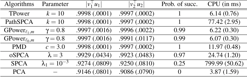
In this experiment, we regard the true model to be successfully recovered when both quanti-ties|v⊤1u1|and|v⊤2u2|are greater than 0.99. Table 1 lists the recovering results by the considered methods. It can be observed that TPower, PathPCA, GPower, PMD and oSPCA all successfully recover the ground truth sparse PC vectors with high rate of success. SPCA frequently fails to re-cover the spares loadings on this data set. The potential reason is that SPCA is initialized with the ordinary principal components which in many random data matrices are far away from the truth sparse solution. Traditional PCA always fails to recover the sparse PC loadings on this data set. The success of TPower and the failure of traditional PCA can be well explained by our sparse recovery result in Theorem 4 (for TPower) in comparison to the traditional eigenvector perturbation theory in Lemma 10 (for traditional PCA), which we have already discussed in §3. However, the success of other methods suggests that it might be possible to prove sparse recovery results similar to The-orem 4 for some of these alternative algorithms. The running time of these algorithms on this data is listed in the last column of Table 1. It can be seen that TPower is among the top efficient solvers.
Algorithms Parameter |v⊤1u1| |v⊤2u2| Prob. of succ. CPU (in ms)
TPower k=10 .9998 (.0001) .9997 (.0002) 1 6.14 (0.76)
PathSPCA k=10 .9998 (.0001) .9997 (.0002) 1 77.42 (2.95)
GPowerℓ1,m γ=0.8 .9997 (.0016) .9996 (.0022) 0.99 6.22 (0.30)
GPowerℓ0,m γ=0.8 .9997 (.0016) .9991 (.0117) 0.99 6.07 (0.30)
PMD c=3.0 .9998 (.0001) .9997 (.0002) 1 11.97 (0.48)
oSPCA λ=3 .9929 (.0434) .9923 (.0483) 0.97 24.74 (1.20)
SPCA λ1=10−3 .9274 (.0809) .9250 (.0810) 0.25 799.99 (50.62)
PCA − .9146 (.0801) .9086 (.0790) 0 3.87 (1.59)
Table 1: The quantitative results on a synthetic data set. The values|v⊤1u1|,|v⊤2u2|, CPU time (in ms) are in format of mean (std) over 500 running.
4.2.3 RESULTSON PITPROPSDATA
The PitPropsdata set (Jeffers, 1967), which consists of 180 observations with 13 measured
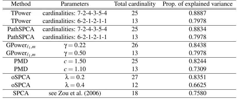
the proportion of adjusted variance (Zou et al., 2006) explained by six components computed with TPower, PathSPCA (d’Aspremont et al., 2008), GPower, PMD, oSPCA and SPCA. From these re-sults we can see that on this relatively simple data set, TPower, PathSPCA and GPower perform quite similarly and are slightly better than PMD, oSPCA and SPCA.
Table 3 lists the six extracted PCs by TPower with cardinality setting 6-2-1-2-1-1. We can see that the important variables associated with the six PCs are exclusive except for the variable “ringb” which is simultaneously selected by PC1 and PC4. The variable “diaknot” is excluded from all the six PCs. The same loadings are also extracted by both PathSPCA and GPower under the parameters listed in Table 2.
Method Parameters Total cardinality Prop. of explained variance
TPower cardinalities: 7-2-4-3-5-4 25 0.8887
TPower cardinalities: 6-2-1-2-1-1 13 0.7978
PathSPCA cardinalities: 7-2-4-3-5-4 25 0.8834
PathSPCA cardinalities: 6-2-1-2-1-1 13 0.7978
GPowerℓ1,m γ=0.22 26 0.8438
GPowerℓ1,m γ=0.50 13 0.7978
PMD c=1.50 25 0.8244
PMD c=1.10 13 0.7309
oSPCA λ=0.2 27 0.8351
oSPCA λ=0.4 12 0.6625
SPCA see Zou et al. (2006) 18 0.7580
Table 2: The quantitative results on thePitPropsdata set. The result of SPCA is taken from Zou et al. (2006).
PCs x1 topd
x2 length
x3 moist
x4 testsg
x5 ovensg
x6 ringt
x7 ringb
x8 bowm
x9 bowd
x10 whorls
x11 clear
x12 knots
x13 diaknot
PC1 .4444 .4534 0 0 0 0 .3779 .3415 .4032 .4183 0 0 0
PC2 0 0 .7071 .7071 0 0 0 0 0 0 0 0 0
PC3 0 0 0 0 1.000 0 0 0 0 0 0 0 0
PC4 0 0 0 0 0 .8569 .5154 0 0 0 0 0 0
PC5 0 0 0 0 0 0 0 0 0 1.000 0 0
PC6 0 0 0 0 0 0 0 0 0 0 0 1.000 0
Table 3: The extracted six PCs by TPower onPitPropsdata set with cardinality setting 6-2-1-2-1-1. Note that in this setting, the extracted significant loadings are non-overlapping except for “ringb”. And the variable “diaknot” is excluded from all the six PCs.
4.2.4 RESULTSON BIOLOGICALDATA
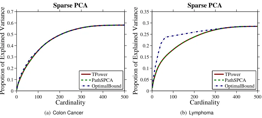
We have also evaluated the performance of TPower on two gene expression data sets, one is the
Colon cancer data from Alon et al. (1999), the other is the Lymphoma data from Alizadeh et al.
to-0 100 200 300 400 500 0
0.1 0.2 0.3 0.4 0.5 0.6 0.7
Cardinality
Propotion of Explained Variance
Sparse PCA
TPower PathSPCA OptimalBound
(a) Colon Cancer
0 100 200 300 400 500
0 0.05 0.1 0.15 0.2 0.25 0.3 0.35
Cardinality
Propotion of Explained Variance
Sparse PCA
TPower PathSPCA OptimalBound
(b)Lymphoma
Figure 2: The variance versus cardinality tradeoff curves on two gene expression data sets. For better viewing, please see the original pdf file.
gether with the result from PathSPCA and the upper bounds of optimal values from d’Aspremont et al. (2008). Note that our method performs almost identical to the PathSPCA which is demon-strated to have optimal or very close to optimal solutions in many cardinalities. The computational time of the two methods on both data sets is comparable and is less than two seconds.
4.2.5 SUMMARY
To summarize this group of experiments on sparse PCA, the basic finding is that TPower performs quite competitively in terms of the tradeoff between explained variance and representation sparsity. The performance is comparable or superior to leading methods such as PathSPCA and GPower. It is observed that TPower, PathSPCA and GPower outperform PMD, oSPCA and SPCA on the benchmark data Pitprops. It is not surprising that TPower and GPower behave similarly because both are power-truncation-type method (see the previous §4.2.1). While strong theoretical guarantee can be established for the TPower method, it remains open to show that PathSPCA and GPower have a similar sparse recovery performance.
4.3 Densestk-Subgraph Finding
It has been shown that the DkS problem is NP hard for bipartite graphs and chordal graphs (Corneil and Perl, 1984), and even for graphs of maximum degree three (Feige et al., 2001). A large body of algorithms have been proposed based on a variety of techniques including greedy al-gorithms (Feige et al., 2001; Asahiro et al., 2002; Ravi et al., 1994), linear programming (Billionnet and Roupin, 2004; Khuller and Saha, 2009), and semidefinite programming (Srivastav and Wolf, 1998; Ye and Zhang, 2003). For generalk, the algorithm developed by Feige et al. (2001) achieves the best approximation ratio ofO(nε)whereε<1/3. Ravi et al. (1994) proposed 4-approximation algorithms for weighted DkS on complete graphs for which the weights satisfy the triangle inequal-ity. Liazi et al. (2008) has presented a 3-approximation algorithm for DkS for chordal graphs. Recently, Jiang et al. (2010) proposed to reformulate DkS as a 1-mean clustering problem and developed a 2-approximation to the reformulated clustering problem. Moreover, based on this re-formulation, Yang (2010) proposed a 1+ε-approximation algorithm with certain exhaustive (and thus expensive) initialization procedure. In general, however, Khot (2006) showed that DkS has no polynomial time approximation scheme (PTAS), assuming that there are no sub-exponential time algorithms for problems in NP.
Mathematically, DkS can be restated as the following binary quadratic programming problem:
max
π∈Rnπ
⊤Wπ, subject toπ∈ {1,0}n,kπk0=k, (8)
whereW is the (non-negative weighted) adjacency matrix ofG. IfGis an undirected graph, then
W is symmetric. IfGis directed, thenW could be asymmetric. In this latter case, from the fact that
π⊤Wπ=π⊤W+W⊤
2 π, we may equivalently solve Problem (8) by replacingWwith
W+W⊤
2 . Therefore, in the following discussion, we always assume that the affinity matrixW is symmetric (or G is undirected).
4.3.1 THETPOWER-DKS ALGORITHM
We propose the TPower-DkS algorithm as an adaptation of TPower to the DkS problem. The process generates a sequence of intermediate vectorsπ0,π1, ...from a starting vectorπ0. At each steptthe vectorπt−1is multiplied by the matrixW, thenπt is set to be the indicator vector of the topkentries
inWπt−1. The TPower-Dks is outlined in Algorithm 2. The convergence of this algorithm can be justified using the same arguments of bounding optimization as described in §2.2.
Algorithm 2:Truncated Power Method for DkS (TPower-DkS)
Input :W ∈Sn+,, initial vectorπ0∈Rn Output :πt
Parameters : cardinalityk∈ {1, ...,n}
Lett=1.
repeat
Computeπt′=Wπt−1.
IdentifyFt=supp(πt′,k)the index set ofπ′twith topkvalues.
Setπt to be 1 on the index setFt, and 0 otherwise.
t←t+1.
Remark 7 By relaxing the constraint π∈ {0,1}n to kπk=√k, we may convert the densest
k-subgraph problem (8) to the standard sparse eigenvalue problem (1) (up to a scaling) and then
directly apply TPower (in Algorithm 1) for solution. Our numerical experience shows that such a relaxation strategy also works satisfactory in practice, although is slightly inferior to TPower-DkS (in Algorithm 2) which directly addresses the original problem.
Remark 8 As aforementioned that the DkS problem is generally NP-hard. The quality of its ap-proximate solution can be measured by the approximation ratio defined as the output objective to the optimal objective. Recently, Jiang et al. (2010) proposed to reformulate DkS as a 1-mean
clus-tering problem and developed a2-approximation to the reformulated clustering problem. Moreover,
based on this reformulation, Yang (2010) proposed a 1+ε-approximation algorithm with certain
exhaustive (and thus expensive) initialization procedure. Provided that W is positive semidefinite with equal diagonal elements, trivial derivation shows that TPower-DkS is identical to the method of Jiang et al. (2010). Therefore, the approximation ratio results from Jiang et al. (2010); Yang (2010) can be shared by TPower-DkS in this restricted case.
Note that in Algorithm 2 we require thatW is positive semidefinite. The motivation of this requirement is to guarantee the convexity of the objective in problem (8), and thus the convergence of Algorithm 2 can be justified by the similar arguments in §2.2. In many real-world DkS problems, however, it is often the case that the affinity matrixW is not positive semidefinite. In this case, the objective is non-convex and thus the monotonicity of TPower-DkS does not hold. However, this complication can be circumvented by instead running the algorithm with the shifted quadratic function:
max
π∈Rnπ
⊤(W+λ˜I
p×p)π, subject toπ∈ {0,1}n,kπk0=k.
where ˜λ>0 is large enough such that ˜W=W+λ˜Ip×p∈Sn+. On the domain of interest, this change only adds a constant term to the objective function. The TPower-DkS, however, produces a different sequence of iterates, and there is a clear tradeoff. If the second term dominates the first term (say by choosing a very large ˜λ), the objective function becomes approximately a squared norm, and the algorithm tends to terminate in very few iterations. In the limiting case of ˜λ→∞, the method will not move away from the initial iterate. To handle this issue, we propose to gradually increase ˜λ
during the iterations and we do so only when the monotonicity is violated. To be precise, if at a time instancet,π⊤t Wπt <π⊤t−1Wπt−1, then we add ˜λIp×ptoWwith a gradually increased ˜λby repeating
the current iteration with the updated matrix untilπ⊤t (W+λ˜Ip×p)πt≥πt⊤−1(W+λIp×p)πt−1,2which impliesπ⊤
t Wπt≥πt⊤−1Wπt−1. 4.3.2 ONINITIALIZATION
Since TPower-DkS is a monotonically increasing procedure, it guarantees to improve the initial pointπ0. Basically, any existing approximation DkS method, for example, greedy algorithms (Feige et al., 2001; Ravi et al., 1994), can be used to initialize TPower-DkS. In our numerical experiments, we observe that by simply settingπ0as the indicator vector of the vertices with the topk(weighted) degrees, our method can achieve very competitive results on all the real-world data sets we have tested on.
4.3.3 RESULTSON WEBGRAPHS
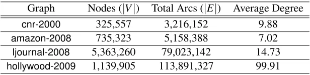
We have tested TPower on four page-level web graphs: cnr-2000, amazon-2008, ljournal-2008,
hollywood-2009, from the WebGraph framework provided by the Laboratory for Web Algorithms.3
We treated each directed arc as an undirected edge. Table 4 lists the statistics of the data sets used in the experiment.
Graph Nodes (|V|) Total Arcs (|E|) Average Degree
cnr-2000 325,557 3,216,152 9.88
amazon-2008 735,323 5,158,388 7.02
ljournal-2008 5,363,260 79,023,142 14.73
hollywood-2009 1,139,905 113,891,327 99.91
Table 4: The statistics of the web graph data sets.
We compare our TPower-DkS method with two greedy methods for the DkS problem. One greedy method is proposed by Ravi et al. (1994) which is referred to as Greedy-Ravi in our experi-ments. The Greedy-Ravi algorithm works as follows: it starts from a heaviest edge and repeatedly adds a vertex to the current subgraph to maximize the weight of the resulting new subgraph; this process is repeated untilkvertices are chosen. The other greedy method is developed by Feige et al. (2001, Procedure 2) which is referred as Greedy-Feige in our experiments. The procedure works as follows: letSdenote thek/2 vertices with the highest degrees inG; letCdenote thek/2 vertices in the remaining vertices with largest number of neighbors inS; returnS∪C.
Figure 3 shows the density value π⊤Wπ/k and CPU time versus the cardinalityk. From the density curves we can observe that oncnr-2000,ljournal-2008andhollywood-2009, TPower-DkS consistently outputs denser subgraphs than the two greedy algorithms, while on amazon-2008, TPower-DkS and Greedy-Ravi are comparable and both are better than Greedy-Feige. For CPU running time, it can be seen from the right column of Figure 3 that Greedy-Feige is the fastest among the three methods while TPower-DkS is only slightly slower. This is due to the fact that TPower-DkS needs iterative matrix-vector products while Greedy-Feige only needs a few degree sorting operations. Although TPower-DkS is slightly slower than Greedy-Feige, it is still quite efficient. For example, on hollywood-2009 which has hundreds of millions of arcs, for each k, Greedy-Feige terminates within about 1 second while TPower terminates within about 10 seconds. The Greedy-Ravi method is however much slower than the other two on all the graphs whenk is large.
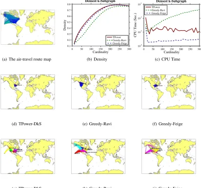
4.3.4 RESULTSON AIR-TRAVELROUTINE
We have applied TPower-DkS to identify subsets of American and Canadian cities that are most easily connected to each other, in terms of estimated commercial airline travel time. The graph4 is of size|V|=456 and|E|=71,959: the vertices are 456 busiest commercial airports in United States and Canada, while the weightwi j of edgeei j is set to the inverse of the mean time it takes
to travel from cityito city jby airline, including estimated stopover delays. Due to the headwind
0 2000 4000 6000 8000 10000 0 10 20 30 40 50 60 70 Cardinality Density Densest k-Subgraph TPower Greedy-Ravi Greedy-Feige
0 2000 4000 6000 8000 10000 10-2 10-1 100 101 102 103 Cardinality
CPU Time (Sec.)
Densest k-Subgraph
TPower Greedy-Ravi Greedy-Feige
(a) cnr-2000
0 2000 4000 6000 8000 10000 3 4 5 6 7 8 9 Cardinality Density Densest k-Subgraph TPower Greedy-Ravi Greedy-Feige
0 2000 4000 6000 8000 10000 10-1 100 101 102 103 Cardinality
CPU Time (Sec.)
Densest k-Subgraph
TPower Greedy-Ravi Greedy-Feige
(b) amazon-2008
0 2000 4000 6000 8000 10000 0 50 100 150 200 250 Cardinality Density Densest k-Subgraph TPower Greedy-Ravi Greedy-Feige
0 2000 4000 6000 8000 10000 100 101 102 103 104 Cardinality
CPU Time (Sec.)
Densest k-Subgraph
TPower Greedy-Ravi Greedy-Feige
(c) ljournal-2008
0 2000 4000 6000 8000 10000 0 500 1000 1500 2000 Cardinality Density Densest k-Subgraph TPower Greedy-Ravi Greedy-Feige
0 2000 4000 6000 8000 10000 10-1 100 101 102 103 104 Cardinality
CPU Time (Sec.)
Densest k-Subgraph
TPower Greedy-Ravi Greedy-Feige
(d) hollywood-2009
effect, the transit time can depend on the direction of travel; thus 36% of the weight are asymmetric. Figure 4(a) shows a map of air-travel routine.
As in the previous experiment, we compare TPower-DkS to Greedy-Ravi and Greedy-Feige on this data set. For all the three considered algorithms, the densities ofk-subgraphs under differ-entk values are shown in Figure 4(b), and the CPU running time curves are given in Figure 4(c). From the former figure we observe that TPower-DkS consistently outperforms the other two greedy algorithms in terms of the density of the extracted k-subgraphs. From the latter figure we can see that TPower-DkS is slightly slower than Greed-Feige but much faster than Greedy-Ravi. Fig-ure 4(d)∼4(f) illustrate the densestk-subgraph withk=30 output by the three algorithms. In each of these three subgraph, the red dot indicates the representing city with the largest (weighted) degree. Both TPower-DkS and Greedy-Feige reveal 30 cities in east US. The former takesClevelandas the representing city while the latterCincinnati. Greedy-Ravi reveals 30 cities in west US and CA and takes Vancouveras the representing city. Visual inspection shows that the subgraph recovered by TPower-DkS is the densest among the three.
After discovering the densestk-subgraph, we can eliminate their nodes and edges from the graph and then apply the algorithms on the reduced graph to search for the next densest subgraph. This se-quential procedure can be repeated to find multiple densestk-subgraphs. Figure 4(g)∼4(i) illustrate sequentially estimated six densest 30-subgraphs by the three considered algorithms. Again, visual inspection shows that our method outputs more geographically compact subsets of cities than the other two. As a quantitative result, the total densities of the six subgraphs discovered by the three algorithms are: 1.14 (TPower-DkS), 0.90 (Greedy-Feige) and 0.99 (Greedy-Ravi), respectively.
5. Conclusion
The sparse eigenvalue problem has been widely studied in machine learning with applications such as sparse PCA. TPower is a truncated power iteration method that approximately solves the non-convex sparse eigenvalue problem. Our analysis shows that when the underlying matrix has sparse eigenvectors, under proper conditions TPower can approximately recover the true sparse solution. The theoretical benefit of this method is that with appropriate initialization, the reconstruction qual-ity depends on the restricted matrix perturbation error at size s that is comparable to the sparsity ¯
k, instead of the full matrix dimension p. This explains why this method has good empirical per-formance. To our knowledge, this is one of the first theoretical results of this kind, although our empirical study suggests that it might be possible to prove related sparse recovery results for some other algorithms we have tested. We have applied TPower to two concrete applications: sparse PCA and the densestk-subgraph finding problem. Extensive experimental results on synthetic and real-world data sets validate the effectiveness and efficiency of the TPower algorithm. To summarize, simply combing power iteration with hard-thresholding truncation provides an accurate and scalable computational method for the sparse eigenvalue problem.
Acknowledgments
(a) The air-travel route map
0 50 100 150 200 250 300 0.1
0.2 0.3 0.4 0.5 0.6 0.7 0.8
Cardinality
Density
Densest k-Subgraph
TPower Greedy-Ravi Greedy-Feige
(b) Density
0 50 100 150 200 250 300 10-4
10-3 10-2 10-1
Cardinality
CPU Time (Sec.)
Densest k-Subgraph
TPower Greedy-Ravi Greedy-Feige
(c) CPU Time
(d) TPower-DkS (e) Greedy-Ravi (f) Greedy-Feige
(g) TPower-DkS (h) Greedy-Ravi (i) Greedy-Feige
Appendix A. Proof Of Theorem 4
Our proof employs several technical tools including the perturbation theory of symmetric eigen-value problem (Lemma 9 and Lemma 10), the convergence analysis of traditional power method (Lemma 11), and the error analysis of hard-thresholding operation (Lemma 12).
We state the following standard result from the perturbation theory of symmetric eigenvalue problem (see, e.g., Golub and Loan, 1996).
Lemma 9 If B and B+U are p×p symmetric matrices, then∀1≤k≤p,
λk(B) +λp(U)≤λk(B+U)≤λk(B) +λ1(U),
whereλk(B)denotes the k-th largest eigenvalue of matrix B.
Lemma 10 Consider set F such that supp(x¯)⊆F with|F|=s. Ifρ(E,s)≤∆λ/2, then the ratio
of the second largest (in absolute value) to the largest eigenvalue of sub matrix AF is no more than
γ(s). Moreover,
kx¯⊤−x(F)k ≤δ(s):=
√
2ρ(E,s)
p
ρ(E,s)2+ (∆λ−2ρ(E,s))2.
Proof We may use Lemma 9 withB=A¯F andU=EF to obtain
λ1(AF)≥λ1(A¯F) +λp(EF)≥λ1(A¯F)−ρ(EF)≥λ−ρ(E,s)
and∀j≥2,
|λj(AF)| ≤ |λj(A¯F)|+ρ(EF)≤λ−∆λ+ρ(E,s).
This implies the first statement of the lemma.
Now letx(F), the largest eigenvector ofAF, beαx¯+βx′, wherekx¯k2=kx′k2=1, ¯x⊤x′=0 and
α2+β2=1, with eigenvalueλ′≥λ−ρ(E,s). This implies that
αAFx¯+βAFx′=λ′(αx¯+βx′),
implying
αx′⊤AFx¯+βx′⊤AFx′=λ′β.
That is,
|β|=|α| x′⊤AFx¯
λ′−x′⊤AFx′ ≤ |α|
|x′⊤AFx¯|
λ′−x′⊤AFx′ =|α|
|x′⊤EFx¯|
λ′−x′⊤AFx′ ≤t|α|,
where t=ρ(E,s)/(∆λ−2ρ(E,s)). This implies that α2(1+t2)≥α2+β2=1, and thus α2≥ 1/(1+t2). Without loss of generality, we may assume thatα>0, because otherwise we can replace
¯
xwith−x¯. It follows that
kx(F)−x¯k2=2−2x(F)⊤x¯=2−2α≤2 √
1+t2−1 √
1+t2 ≤
2t2
1+t2. This implies the desired bound.
Lemma 11 Let y be the eigenvector with the largest (in absolute value) eigenvalue of a symmetric
matrix A, and letγ<1be the ratio of the second largest to largest eigenvalue in absolute values.
Given any x such thatkxk=1and y⊤x>0; let x′=Ax/kAxk, then
|y⊤x′| ≥ |y⊤x|[1+ (1−γ2)(1−(y⊤x)2)/2].
Proof Without loss of generality, we may assume thatλ1(A) =1 is the largest eigenvalue in absolute value, and|λj(A)| ≤γwhen j>1. We can decomposex asx=αy+βy′, wherey⊤y′ =0, kyk=
ky′k=1, andα2+β2=1. Then|α|=|x⊤y|. Letz′=Ay′, thenkz′k ≤γandy⊤z′=0. This means
Ax=αy+βz′, and
|y⊤x′|=|y⊤Ax| kAxk =
|α| p
α2+β2kz′k2 ≥
|α| p
α2+β2γ2 =p |y⊤x|
1−(1−γ2)(1−(y⊤x)2) ≥|y⊤x|[1+ (1−γ2)(1−(y⊤x)2)/2].
The last inequality is due to 1/√1−z≥1+z/2 forz∈[0,1). This proves the desired bound.
The following lemma quantifies the error introduced by the truncation step in TPower.
Lemma 12 Consider x with supp¯ (x¯) =F and¯ k¯ =|F¯|. Consider y and let F =supp(y,k) be the
indices of y with the largest k absolute values. Ifkx¯k=kyk=1, then
|Truncate(y,F)⊤x¯| ≥ |y⊤x¯| −(k¯/k)1/2min
q
1−(y⊤x¯)2,(1+ (k¯/k)1/2) (1
−(y⊤x¯)2)
.
Proof Without loss of generality, we assume that y⊤x¯=∆>0. We can also assume that ∆>
p¯
k/(k¯+k) because otherwise the right hand side is smaller than zero, and thus the result holds trivially.
LetF1=F¯\F, and F2=F¯∩F, andF3=F\F¯. Now, let ¯α=kx¯F1k, ¯β=kx¯F2k, α=kyF1k,
β=kyF2k, and γ=kyF3k. letk1 =|F1|, k2=|F2|, andk3 =|F3|. It follows thatα 2/k
1≤γ2/k3. Therefore
∆2≤[αα¯ +ββ¯ ]2≤α2+β2≤1−γ2≤1−(k3/k1)α2. This implies that
α2≤(k1/k3)(1−∆2)≤(k¯/k)(1−∆2)<∆2, (9)
where the second inequality follows from ¯k≤kand the last inequality follows from the assumption
∆>pk¯/(k¯+k). Now by solving the following inequality for ¯α
αα¯+p1−α2p1−α¯2≥αα¯+ββ¯≥∆ under the condition∆>α≥αα¯, we obtain that
¯
α≤α∆+p1−α2p1−∆2≤minh1,α+p1−∆2i≤minh1,(1+ (k¯/k)1/2)p
where the second inequality follows from the Cauchy-Schwartz inequality and∆≤1,√1−α2≤1, while the last inequality follows from (9). Finally,
|y⊤x¯| − |Truncate(y,F)⊤x¯| ≤ |(y−Truncate(y,F))⊤x¯|
≤ αα¯ ≤(k¯/k)1/2minq1−(y⊤x¯)2,(1+ (k¯/k)1/2) (1−(y⊤x¯)2)
,
where the last inequality follows from (9) and (10). This leads to the desired bound.
Next is our main lemma, which says each step of sparse power method improves eigenvector estimation.
Lemma 13 Assume that k≥k. Let s¯ =2k+k. If¯ |x⊤
t−1x¯|>θ+δ(s), then
q
1− |xˆt⊤x¯| ≤µ q
1− |x⊤t−1x¯|+√10δ(s).
Proof LetF=Ft−1∪Ft∪supp(x¯). Consider the following vector
˜
xt′=AFxt−1/kAFxt−1k, (11)
whereAF denotes the restriction ofAon the rows and columns indexed byF. We note that replacing
x′t with ˜x′t in Algorithm 1 does not affect the output iteration sequence{xt}because of the sparsity
of xt−1 and the fact that the truncation operation is invariant to scaling. Therefore for notation simplicity, in the following proof we will simply assume thatx′t is redefined asxt′=x˜t′according to (11).
Without loss of generality and for simplicity, we may assume that x′⊤t x(F)≥0 andxt⊤−1x¯≥ 0, because otherwise we can simply do appropriate sign changes in the proof. We obtain from Lemma 11 that
x′⊤t x(F)≥x⊤t−1x(F) [1+ (1−γ(s)2)(1−(x⊤t−1x(F))2)/2].
This implies that
[1−x′⊤t x(F)]≤[1−xt⊤−1x(F)] [1−(1−γ(s)2)(1+xt⊤−1x(F))(x⊤t−1x(F))/2] ≤[1−xt⊤−1x(F)] [1−0.5θ(1+θ)(1−γ(s)2)],
where in the derivation of the second inequality, we have used Lemma 10 and the assumption of the lemma that impliesx⊤t−1x(F)≥xt⊤−1x¯−δ(s)≥θ. We thus have
kxt′−x(F)k ≤ kxt−1−x(F)k
q
1−0.5θ(1+θ)(1−γ(s)2). Therefore using Lemma 10, we have
kx′t−x¯k ≤ kxt−1−x¯k
q
1−0.5θ(1+θ)(1−γ(s)2) +2δ(s). This is equivalent to
q
1− |x′t⊤x¯| ≤
q
1− |x⊤t−1x¯|
q
Next we can apply Lemma 12 and usek≥k¯to obtain
q
1− |xˆ⊤t x¯| ≤
q
1− |xt′⊤x¯|+ ((k¯/k)1/2+k¯/k)(1− |x′
t⊤x¯|2)
≤
q
1− |xt′⊤x¯|
q
1+2((k¯/k)1/2+k¯/k) ≤ µ
q
1− |xt−1⊤x¯|+ √
10δ(s).
This proves the second desired inequality.
We are now in the position to prove Theorem 4.
Proof of Theorem 4:
Let us distinguish the following two complementary cases:
Case I:θ+δ(s)>1−10δ(s)2/(1−µ)2. In this case, we have thatx⊤
0x¯≥θ+δ(s)>1−10δ(s)2/(1−
µ)2which implies the inequality (5).
Case II:θ+δ(s)≤1−10δ(s)2/(1−µ)2. In this case, we first prove by induction that for allt≥0,
x⊤t x¯≥θ+δ(s). This is obviously hold fort=0. Assume that |xt⊤−1x¯| ≥θ+δ(s). Let us further distinguish the following two cases:
(a)
q
1− |xt⊤−1x¯| ≥√10δ(s)/(1−µ). From Lemma 13 we obtain that
q
1− |xt⊤x¯| ≤ q
1− |xˆ⊤t x¯| ≤µ q
1− |x⊤t−1x¯|+√10δ(s)≤
q
1− |xt⊤−1x¯|,
where the first inequality follows from |x⊤t x¯|=|xˆ⊤t x¯|/kxˆtk ≥ |xˆt⊤x¯|. This implies |xt⊤x¯| ≥
|xt⊤−1x¯| ≥θ+δ(s). (b)
q
1− |xt⊤−1x¯|<√10δ(s)/(1−µ). Based on the previous argument we have
q
1− |x⊤t x¯| ≤µ q
1− |x⊤t−1x¯|+√10δ(s)<√10δ(s)/(1−µ),
which implies that|xt⊤x¯|>1−10δ(s)2/(1−µ)2≥θ+δ(s).
In both cases (a) and (b), we have |x⊤t x¯| ≥θ+δ(s)and this finishes the induction. Therefore, by recursively applying Lemma 13 we have that for allt≥0
q
1− |x⊤t x¯| ≤µt q
1− |x⊤0x¯|+√10δ(s)/(1−µ),
which is inequality (6). This completes the proof.
References
A. Alon, N. Barkai, D. A. Notterman, K. Gish, S. Ybarra, D. Mack, and A. J. Levine. Broad patterns of gene expression revealed by clustering analysis of tumor and normal colon tissues probed by oligonucleotide arrays. Cell Biology, 96:6745–6750, 1999.
A. A. Amini and M. J. Wainwright. High-dimensional analysis of semidefinite relaxiation for sparse principal components. Annals of Statistics, 37:2877–2921, 2009.
Y. Asahiro, R. Hassin, and K. Iwama. Complexity of finidng dense subgraphs. Discrete Applied
Mathematics, 211(1-3):15–26, 2002.
A. Billionnet and F. Roupin. A deterministic algorithm for the densest k-subgraph problem using linear programming. Technical report, Technical Report, No. 486, CEDRIC, CNAM-IIE, Paris, 2004.
T. Cai, Z. Ma, and Y. Wu. Sparse pca: Optimal rates and adaptive estimation. 2012. URLarxiv. org/pdf/1211.1309v1.pdf.
E. J. Candes and T. Tao. Decoding by linear programming. IEEE Transactions on Information
Theory, 51:4203–4215, 2005.
D. G. Corneil and Y. Perl. Clustering and domination in perfect graphs. Discrete Applied
Mathe-matics, 9:27–39, 1984.
A. d’Aspremont, L. El Ghaoui, M. I. Jordan, and G. R. G. Lanckriet. A direct formulation for sparse pca using semidefinite programming. SIAM Review, 49:434–448, 2007.
A. d’Aspremont, F. Bach, and L. El Ghaoui. Optimal solutions for sparse principal component analysis. Journal of Machine Learning Research, 9:1269–1294, 2008.
U. Feige, G. Kortsarz, and D. Peleg. The densek-subgraph problem.Algorithmica, 29(3):410–421, 2001.
X. Geng, T. Liu, T. Qin, and H. Li. Feature selection for ranking. InProceedings of the 30th Annual
International ACM SIGIR Conference (SIGIR’07), 2007.
D. Gibson, R. Kumar, and A. Tomkins. Discovering large dense subgraphs in massive graphs. In
Proceedings of the 31st International Conference on Very Large Data Bases (VLDB’05), pages
721–732, 2005.
G. H. Golub and C.F. Van Loan.Matrix Computations. Johns Hopkins University Press, Baltimore, MD, third edition, 1996.
J. Jeffers. Two case studies in the application of principal components. Applied Statistics, 16(3): 225–236, 1967.
P. Jiang, J. Peng, M. Heath, and R. Yang. Finding densest k-subgraph via 1-mean clustering and low-dimension approximation. Technical report, 2010.
I. M. Johnstone. On the distribution of the largest eigenvalue in principal components analysis.
I. T. Jolliffe, N. T. Trendafilov, and M. Uddin. A modified principal component technique based on the lasso. Journal of Computational and Graphical Statistics, 12(3):531–547, 2003.
M. Journ´ee, Y. Nesterov, P. Richt´arik, and Rodolphe Sepulchre. Generalized power method for sparse principal component analysis. Journal of Machine Learning Research, 11:517–553, 2010.
S. Khot. Ruling out ptas for graph min-bisection, dense k-subgraph, and bipartite clique. SIAM
Journal on Computing, 36(4):1025–1071, 2006.
S. Khuller and B. Saha. On finding dense subgraphs. In Proceedings of the 36th International
Colloquium on Automata, Languages and Programming (ICALP’09), pages 597–608, 2009.
R. Kumar, P. Raghavan, S. Rajagopalan, and A. Tomkins. Trawling the web for emerging cyber-communities. InProceedings of the 8th World Wide Web Conference (WWW’99), pages 403–410, 1999.
M. Liazi, I. Milis, and V. Zissimopoulos. A constant approximation algorithm for the densest k-subgraph problem on chordal graphs. Information Processing Letters, 108(1):29–32, 2008.
Z. Ma. Sparse principal component analysis and iterative thresholding. Annals of Statistics, to appear, 2013.
L. Mackey. Deflation methods for sparse pca. InProceedings of the 22nd Annual Conference on
Neural Information Processing Systems (NIPS’08), 2008.
J. Mairal, F. Bach, J. Ponce, and G. Sapiro. Online learning for matrix factorization and sparse coding. Journal of Machine Learning Research, 11:10–60, 2010.
B. Moghaddam, Y. Weiss, and S. Avidan. Generalized spectral bounds for sparse lda. InProceedings
of the 23rd International Conference on Machine Learning (ICML’06), pages 641–648, 2006.
D. Paul and I.M. Johnstone. Augmented sparse principal component analysis for high dimensional
data. 2012. URLarxiv.org/pdf/1202.1242v1.pdf.
S. S. Ravi, D. J. Rosenkrantz, and G. K. Tayi. Heuristic and special case algorithms for dispersion problems. Operations Research, 42:299–310, 1994.
D. Shen, H. Shen, and J.S. Marron. Consistency of sparse pca in high dimension, low sample size contexts. Journal of Multivariate Analysis, 115:317–333, 2013.
H. Shen and J. Z. Huang. Sparse principal component analysis via regularized low rank matrix approximation. Journal of Multivariate Analysis, 99(6):1015–1034, 2008.
A. Srivastav and K. Wolf. Finding dense subgraphs with semidefinite programming. In Proceed-ings of International Workshop on Approximation Algorithms for Combinatorial Optimization
(APPROX’98), pages 181–191, 1998.
R. Tibshirani. Regression shrinkage and selection via the lasso. Journal of the Royal Statistical
D. M. Witten, R. Tibshirani, and T. Hastie. A penalized matrix decomposition, with applications to sparse principal components and canonical correlation analysis. Biostatistics, 10(3):515–534, 2009.
R. Yang. New approximation methods for solving binary quadratic programming problem. Techni-cal report, Master Thesis, Department of Industrial and Enterprise Systems Engineering, Univer-sity of Illnois at Urbana-Champaign, 2010.
Y. Y. Ye and J. W. Zhang. Approximation of dense-n/2-subgraph and the complement of min-bisection. Journal of Global Optimization, 25:55–73, 2003.
H. Zou, T. Hastie, and R. Tibshirani. Sparse principal component analysis. Journal of