Simulation of Coal Gasification Process Inside a Two-Stage Gasifier

ScholarWorks@UNO

ScholarWorks@UNO

University of New Orleans Theses and

Dissertations Dissertations and Theses

12-17-2004

Simulation of Coal Gasification Process Inside a Two-Stage

Simulation of Coal Gasification Process Inside a Two-Stage

Gasifier

Gasifier

Armin Silaen

University of New Orleans

Follow this and additional works at: https://scholarworks.uno.edu/td

Recommended Citation Recommended Citation

Silaen, Armin, "Simulation of Coal Gasification Process Inside a Two-Stage Gasifier" (2004). University of New Orleans Theses and Dissertations. 198.

https://scholarworks.uno.edu/td/198

This Thesis is protected by copyright and/or related rights. It has been brought to you by ScholarWorks@UNO with permission from the rights-holder(s). You are free to use this Thesis in any way that is permitted by the copyright and related rights legislation that applies to your use. For other uses you need to obtain permission from the rights-holder(s) directly, unless additional rights are indicated by a Creative Commons license in the record and/or on the work itself.

SIMULATION OF

COAL GASIFICATION PROCESS INSIDE A TWO-STAGE GASIFIER

A Thesis

Submitted to the Graduate Faculty of the University of New Orleans

in Partial fulfillment of the requirement for the degree of

Master of Science in

The Department of Mechanical Engineering

by

Armin K. Silaen

B.S. University of New Orleans, 2002

ii

ACKNOWLEDGEMENTS

I would like to express my sincere gratitude to my advisor, Dr. Ting Wang, for his

support, guidance, and patience during the entire period of this study. His willingness to

give his time, insight, wisdom, and interest for this study made this work a success.

I would also like to thank Dr. Carsie A. Hall and Dr. Martin J. Guillot for taking

the time to serve on my thesis defense committee.

I acknowledge all Energy Conversion & Conservation Center (ECCC) personnel.

Special thanks to Dr. Xianchang Li and Mr. Raja Saripalli for their help and advice.

I thank my friends for their friendship and support. Finally, I am grateful for my

mother and late father, to whom I dedicate this work, and my siblings for their

iii

TABLE OF CONTENTS

LIST OF FIGURES ...v

LIST OF TABLES ...viii

NOMENCLATURE ... ix

ABSTRACT... xi

CHAPTER 1. INTRODUCTION ...1

1.1 Background ...1

1.2 Literature ...2

1.2.1. Basic Gasification Reactions ...2

1.2.2. Gasification Methods ...3

1.3 Research and Development (R&D) in Gasification Industry ...17

1.4 Objectives...18

2. COMPUTATIONAL MODEL...19

2.1 Assumptions...21

2.2 Governing Equations ...21

2.3 Turbulence Model...23

2.4 Radiation Model...28

2.5 Combustion Model...29

2.6 Boundary Conditions ...33

3. COMPUTATIONAL PROCESS ...36

3.1 Solution Methodology ...36

3.2 Computational Grid ...37

3.3 Numerical Procedure...37

3.4 Gas temperature and species fractions for three different grids...44

4. RESULTS AND DISCUSSIONS...46

4.1 Baseline Case ...47

4.2 Effects of Coal Mixture (Slurry vs. Powder) ...57

4.3 Effects of Wall Cooling (Case 3) ...61

iv

5. CONCLUSIONS...78

REFERENCES ...82

APPENDICES ...83

A. Application of FLUENT code...84

B. Geometry Generation and Meshing ...109

v

LIST OF FIGURES

Figure 1.1 Schematic of a KRW fluidized-bed gasifier (US Department of Energy/

1996). ...6

Figure 1.2 Schematic of a Lurgy dry ash moving-bed gasifier. ...8

Figure 1.3 Schematic of Texaco entrained-flow gasifier (US Department of Energy, 2000(a)). ...11

Figure 1.4 Schematic of a Shell entrained-flow gasifier (From Shell commercial Brochure). ...13

Figure 1.5 Schematic of E-Gas entrained-flow gasifier (US Department of Energy, 2000(c)). ...14

Figure 2.1 Schematic of a two-stage entrained- flow gasifier configuration. ...20

Figure 2.2 Boundary conditions for the baseline case of the generic two-stage entrained-flow gasifier. ...34

Figure 3.1 Basic program structure of FLUENT code. ...39

Figure 3.2 Meshed geometry for the REI gasifier. ...40

Figure 3.3 Overview of the segregated solution method...41

Figure 4.1 Axial distributions of the gas temperature and the gas mole fraction at the center vertical plane in the oxygen-blown gasifier with coal-slurry fuel (Case 1)...51

Figure 4.2 Distributions of the gas temperature and the gas mole fraction at different horizontal planes in the oxygen-blown gasifier with coal-slurry fuel (Case 1)...52

Figure 4.3 Distribution of gas temperature and gas mole fraction at lower inlet level for oxyge n-blown gasifier with coal-slurry fuel (Case 1). ...53

vi

gasifier height for oxygen-blown gasifier with coal-slurry fuel (Case 1)...55

Figure 4.6 Midplane axial distributions of the gas temperature and the gas mole

fraction in the oxygen-blown gasifier with coal powder fuel (Case 2)...56

Figure 4.7 Mass-weighted average gas temperature and mole fraction along the

gasifier height for oxygen-blown gasifier with coal powder fuel (Case 2). .59

Figure 4.8 Mass-weighted average gas temperature and mole fraction along the

gasifier height for gasifier with wall cooling (Case 3). ...62

Figure 4.9 Mass-weighted average gas temperature and mole fraction along the gasifier height for Case 4 with 50-50 equal coal distribution between

two stages (Case 4). ...64

Figure 4.10 Mass-weighted average gas temperature and mole fraction along the

gasifier height for gasifier with one-stage coal injection (Case 8). ...64

Figure 4.11 Mass-weighted average gas temperature and mole fraction along the

gasifier height for air-blown gasifier (Case 5). ...66

Figure 4.12 Lower injector configurations of (a) Case 6 and (b) Case 7. ...68

Figure 4.13 Velocity vectors on the center vertical plane for gasifier with the first

stage injectors position horizontally (Case 1). ...69

Figure 4.14 Velocity vectors on the center vertical plane for gasifier with the first

stage injectors tilted 30° downward (Case 6). ...70

Figure 4.15 Velocity vectors on the center vertical plane for gasifier with the first

stage injectors tilted 30° upward (Case 7). ...71

Figure 4.16 Flow path lines for gasifier with the first stage injectors horizontal

(Case 1). ...73

Figure 4.17 Flow path lines for gasifier with the first stage injectors tilted 30°

downward (Case 6). ...74

Figure 4.18 Flow path lines for gasifier with the first stage injectors tilted 30°

upward (Case 7). ...75

Figure 4.19 Mass-weighted average gas temperature and mole fraction along the gasifier height for gasifier with the first stage injectors tilted 30°

vii

Figure 4.20 Mass-weighted average gas temperature and mole fraction along the gasifier height for gasifier with the first stage injectors tilted 30°

viii

LIST OF TABLES

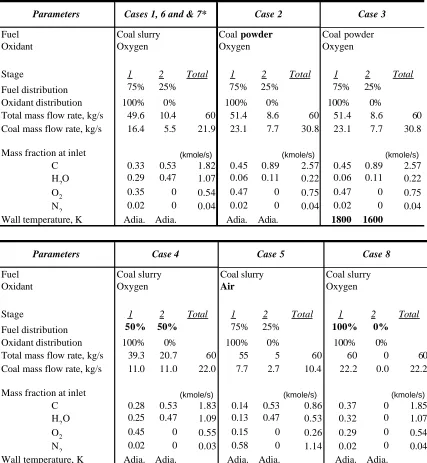
Table 2.1 Parameters and operating conditions for simulated cases...35

Table 3.1 Gas temperature and species fractions for three different grids...45

Table 4.1 Parameters and operating conditions for simulated cases...48

ix

NOMENCLATURE

a local speed of sound (m/s)

c concentration (mass/volume, moles/volume)

cp heat capacity at constant pressure (J/kg-K) cv heat capacity at constant volume (J/kg-K) D mass diffusion coefficient (m2/s)

DH hydraulic diameter (m)

Dij mass diffusion coefficient (m2/s) Dt turbulent diffusivity (m2/s)

E total energy (J)

g gravitational acceleration (m/s2)

G incident radiation

Gr Grashof number (L3.ρ2.g.β.∆T/µ2)

H total enthalpy (W/m2-K)

h species enthalpy (W/m2-K)

J mass flux; diffusion flux (kg/m2-s)

k turbulence kinetic energy (m2/s2)

k thermal conductivity (W/m-K)

m mass (kg)

MW molecular weight (kg/kgmol)

M Mach number

p pressure (atm)

Pr Prandtl number (ν/α)

q heat flux

qr radiation heat flux R universal gas constant

x

t time (s)

T temperature (K)

U mean velocity (m/s)

X mole fraction (dimensionless)

Y mass fraction (dimensionless)

x, y, z coordinates

Greek letter

β coefficient of thermal expansion (K-1)

ε turbulence dissipation (m2/s3)

εw wall emissivity

κ von Karman constant

µ dynamics viscosity (kg/m-s)

µk turbulent viscosity (kg/m-s)

v kinematic viscosity (m2/s)

v’ stoichiometric coefficient of reactant

v” stoichiometric coefficient of product

ρ density (kg/m3)

ρw wall reflectivity

σ Stefan-Boltzmann constant

σs scattering coefficient τ stress tensor (kg/m-s2)

Subscript

i reactant i

j product j

xi ABSTRACT

Gasification is a very efficient method of producing clean synthetic gas (syngas)

which can be used as fuel for electric generation or chemical building block for

petrochemical industries. This study performs detailed simulations of coal gasification

process inside a generic two-stage entrained-flow gasifier to produce syngas carbon

monoxide and hydrogen. The simulations are conducted using the commercial

Computational Fluid Dynamics (CFD) solver FLUENT. The 3-D Navier-Stokes

equations and seven species transport equations are solved with eddy-breakup

combustion model. Simulations are conducted to investigate the effects of coal mixture

(slurry or dry), oxidant (oxygen-blown or air-blown), wall cooling, coal distribution

between the two stages, and the feedstock injection angles on the performance of the

gasifier in producing CO and H2. The result indicates that coal-slurry feed is preferred

over coal-powder feed to produce hydrogen. On the other hand, coal-powder feed is

preferred over coal-slurry feed to produce carbon monoxide. The air-blown operation

yields poor fuel conversion efficiency and lowest syngas heating value. The two-stage

design gives the flexibility to adjust parameters to achieve desired performance. The

horizontal injection design gives better performance compared to upward and downward

CHAPTER ONE

INTRODUCTION

1.1 Background

Gasification is the process of converting various carbon-based feedstocks to clean

synthetic gas (syngas), which is primarily a mixture of hydrogen (H2) and

carbon-monoxide (CO). This conversion is achieved through the reaction of the feedstock with

oxygen and steam at high temperature and pressure with only less than 30% of the

required oxygen for complete combustion being provided. The syngas produced can be

used as a fuel, usually as a fuel for boilers or gas turbines to generate electricity, or can be

used to make a synthetic natural gas hydrogen gas or other chemical products. The

gasification technology is applicable to any type of carbon-based feedstock, such as coal,

natural gas, heavy refinery residues, petroleum coke, biomass, and municipal wastes.

The gas produced from coal gasification can be used for syngas or as a source for

methanol and hydrogen, which are used in the manufacturing process of ammonia or

hydrogenation applications in refineries. Another usage of syngas, which is gaining more

popularity recently, is using syngas as fuel in electricity generation by employing the

Integrated Gasification Combined Cycle (IGCC). The syngas produced in the gasifier is

cleaned and used as a fuel for gas turbines. The gas is burned with compressed air in the

combustor of the gas turbine. The high pressure and hot gases produced in the combustor

The hot exhaust gases from the gas turbine are sent to a boiler that heats water

producing steam that expands through a steam turbine to drive another electric

generator.

IGCC plants can achieve efficiencies of about 50% and low emissions, compared

to 43-45% efficiencies and high emissions for regular or critical pulverized coal

combustion power plants. Gasification integrated in IGCC is considered a clean and

efficient alternative to coal combustion for power generation. The high-pressure and

high-temperature syngas from the gasifier can especially take advantage of the new

generation of advanced turbine systems (ATS), which require high compression ratio and

high turbine inlet temperature to produce up to 60% combined cycle efficiency.

Furthermore, the syngas stream can also be tapped to produce methanol and hydrogen.

1.2 Literature Survey

1.2.1 Basic Gasification Reactions

Coal gasification reactions occur when coal is heated with limited oxygen and

usually steam in a gasification reaction chamber. The main global reactions in a

gasification process are as follows:

Heterogeneous (solid and gas) phase

C(s) + ½ O2→ CO ∆H°R = -110.5 MJ/kmol (R1.1)

C(s) + CO2 → 2CO ∆H°R = +172.0 MJ/kmol (R1.2)

(Gasification, Boudouard reaction)

C(s) + H2O(g) → CO + H2 ∆H°R*= +131.4 MJ/kmol (R1.3)

Homogenous gas phase

CO + ½ O2→ CO2 ∆H°R = -283.1 MJ/kmol (R1.4)

CO + H2O(g) → CO2 + H2 ∆H°R = -41.0 MJ/kmol (R1.5)

(Watershift)

Reactions given in R1.1 and R1.4 are two exothermic reactions that provide the

complete energy for the gasification. Based on these global reactions, approximately

22% of the stoichiometric oxygen is required to provide sufficient energy for gasification

reactions. In real applications, 25~30% of the stoichiometric oxygen is provided to

ensure high-efficient carbon conversion.

Partial combustion occurs when the coal mixes with oxygen (R1.1). The energy

released from (R1.1) also heats up any coal that has not burned. When the coal is heated

without oxygen, it undergoes pyrolysis during which phenols and hydrocarbon gases are

released. At the same time, char gasification (R1.2) takes place and releases CO. If a

significant amount of steam exists, gasification (R1.3) and water shift reaction (R1.5)

occur and release H2.

1.2.2 Gasification Methods

The formation of volatile components from coal was observed in the 17th century.

Murdoch used partial gasification to produce coal gas (town’s gas) for gas lighting in

1797, which led to a major industry in many countries. In the mid-19th century, Siemens

step is also gasified.. Oxygen gasification, where pure oxygen is used, was introduced

around 1925 as a means of producing a high-calorific-value town’s gas.

As technology progressed, the next phase was the development of gasification to

meet the needs of the petroleum industry. The goal was to produce synthetic gas or

substitute natural gas for

• synthesis of gasoline,

• hydrogen for refinery purposes,

• synthetic, sulfur-free, diesel fuel, and

• chemical feedstocks for methanol and amonia were emphasised.

The next development was the power generation using gas turbines. The current

preferred choice of fuel for gas turbines is natural gas. However, this may not be the

most economic choice as future natural gas prices rise. . On the other hand, coal has a

reserve of more than 250 years and the cost of coal is expected to be low for many years

to come. The use of syngas produced from coal gasification reactions as a fuel for gas

turbines has led to the interest and development of coal gasification technology.

Commercial gasifiers have been extensively studied and can be classified based

on flow speeds, feedstock feeding direction, and oxidant feeds. Based on the flow

speeds, gasifiers are classified as:

a. Fluidized-bed gasifier

b. Moving-bed gasifier

c. Entrained-flow gasifier

Based on the direction of feedstock feeding, gasifiers are divided into:

b. Counter-current: the coal and the oxidant move in opposite directions.

c. Updraft: the oxidant is supplied from the bottom, and syngas is extracted on the

top of the gasifier.

d. Downdraft: the oxidant is supplied from the top, and syngas is extracted fromthe

bottom.

Based on the oxidant feed, gasifiers are categorized into:

a. Oxygen blown

b. Air blown

Each type of gasifier, in terms of the flow speed, is discussed briefly below.

a) Fluidized-Bed Gasifier

The flow speed in a fluidized-bed gasifier is about 0.9 m/s. Figure 1.1 shows the

schematic of a fluidized-bed gasifier. Due to the low flow speed, a fluidized-bed gasifier

has long residence time (several minutes). Coal particles with diameters less than 5 mm

are thoroughly mixed with steam and oxygen at the lower part of the reactor. The syngas

formed from the gasification reaction leaves the reactor from the top. The fluidized-bed

gasifier is operated at a constant low temperature, which is below the ash fusion

temperature to avoid agglomeration and clinker formation in the fluidized bed. The

advantage that the fluidized-bed gasifier has over the moving-bed gasifier is the small

temperature difference between the fuel particles and the oxidant due to the thorough

mixing, which results in higher efficiency. Fluidized-bed gasifiers have mid-size

capacity with an operating temperatureof 870-1038°C (1600-1900°F). This small range

of operating temperature is the biggest drawback to fluidized-bed gasifiers. The

enough to avoid formation of tar. Currently, there are 3 types of high-pressure

fluidized-bed gasifier (Kellogg KRW, HT Winkler and U Gas)and one type of low-pressure

fluidized-bed gasifier (Winkler) available commercially.

b) Moving-Bed Gasifier

In a typical moving-bed gasifier, coal is fed into the reactor from the top while

steam and oxygen are fed at the bottom. Steam and oxygen react with coal as they move

up the reactor to form syngas, which then exits from the top. Compared to other types of

gasifiers, the moving-bed gasifier produces the highest heating value fuel gas and

requires the least amount of oxygen. However, a non-uniform mixing and temperature

distribution is a disadvantage; therefore, very high temperature to maintain the

equilibrium of the gasification reaction is required. Due to the countercurrent operation,

there is a significant temperature drop in the reactor and a significant temperature

difference of coal and of gas. This means coal particles and gasses do not mix

thoroughly and results in low efficiency. A moving-bed gasifier can be operated either as

dry-ash bed or slagging bed, depending on temperature and the steam/oxygen ratio

injected into the gasifier. The operating temperature for a slagging bed ranges from

430°C to 1540°C (800-2800°F). The temperature in the reactor must be higher than the

ash melting temperature before quenching is applied. The by-products, tar and liquid

volatile, flow down to the slagging area and decompose. Slagging bed is usually used

with fine coal particles, and dry-ash bed is usuallyused for coarse coal particles. The

design operating temperature for a dry ash bed ranges from 430°C to 1095°C

(800-2000°F), which is below the ash melting temperature.

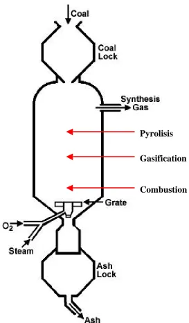
Figure 1.2 shows the schematic of a Lurgi dry ash moving-bed gasifier. A Lurgi

gasifier is a high-pressure and dry-fed moving-bed gasifier. Coal with a diameter

between ¼” to 2” (6~50 mm) is fed from the top of the gasifier through a lock hopper.

Combustion Gasification Pyrolisis

Figure 1.2 Schematic of a Lurgi dry ash moving-bed gasifier.

gasifier. The temperature in the combustion region (bottom part) is around 2000°F, and

the temperature of raw syngas leaving the gasifier from the top is approximately

be injected into the bottom of the gasifier to keep the temperature lower than the melting

point of ash.

Among different types of gasifiers, moving-bed gasifier has the longest history

and is the most widely used commercially. Some examples of moving-bed gasifier are

high-pressure Lurgi dry ash gasifier, British Gas Lurgi (BGL) slagging gasifier, and

low-pressure Wellman Balusha gasifier. Lurgi’s are the predominant gasifiers used by the

South African Coal, Oil, and Gas Corporation (SASOL) to produces a variety of

chemicals and syngas from coal. Although Lurgi is widely used, relatively low capacity

and the inability to handle fine coal powders limit its application. On the other hand,

BGL, co-developed by British Gas and Lurgi, is well fitted to anthracite, and there are

commercial applications showing success.

c) Entrained-Bed Gasifier

The flow speed in an entrained-bed gasifier is the highest among all gasifiers, and

the flow resident time is about 3~5 seconds. Very fine coal particles with diameters less

than 0.13 mm are injected into the reactor together with steam and oxygen. Coal

particles mix and react thoroughly with steam and oxygen in the gasifier, and the syngas

produced exits through the outlet. The operating temperature is high, ranging between

930-1650°C, making efficiency very high. Because the temperature is above the melting

point of ash, most of the ash forms slag and is discharged from the bottom of the gasifier.

The temperature distribution is pretty uniform, and there is nearly no temperature

difference between gas and syngas. The entrained-bed gasifier produces a better mixing

fluidized-bed gasifiers. This makes it widely used in power generation plant. However,

an entrained-bed gasifier does have disadvantages as it requires the highest amount of O2

and produces the lowest heating values gas. Entrained-flow gasifiers predominantly used

in commercial applications are Texaco*, E-Gas**, Shell, Prenflo, and GSP. The first three

gasifiers are briefly described below.

Figure 1.3 shows a schematic of a Texaco gasifier. The Texaco gasifier is a

single-stage, high-pressure, oxygen-blown, downward firing entrained gasifier.

Coal-water slurry and oxygen enters the hot gasifier from the top. The mass fraction of coal in

the coal-water slurry is 60-70%, and the oxidant is 95% pure oxygen. At a temperature

of about 1500°C (2700°F), gasification occurs rapidly. The coal slurry reacts with

oxygen to produce syngas and molten ash. The hot syngas flows downward into a radiant

syngas cooler or a water quench section where high-pressure steam is produced. The

syngas passes over the surface of a pool of water at the bottom of the radiant syngas

cooler and exits the reactor. The slag drops into the water pool and cools down. It is

then fed from the radiant syngas cooler sump to a lock hopper. The black water flowing

out with the slag is separated and recycled after processing in a dewatering system.

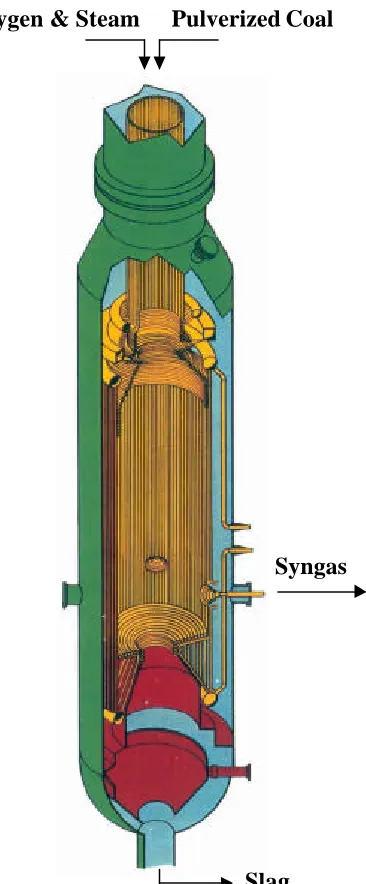
The Shell gasifier is a high-pressure, dry-fed, oxygen-blown, downdraft

entrained-flow gasifiers. Figure 1.4 illustrates a schematic of the Shell gasifier.

Pulverized, dried coal is fed into the high-pressure vessel with transport gas through a

lock hopper system. The transport gas is usually nitrogen. Steam and oxygen enter into

*

Texaco: Texaco Inc merged with Chevron Corp to form ChevronTexaco in 2001. The ChevronTexaco gasificatin division was purchased by General Electric in 2004.

**

Figure 1.3 Schematic of Texaco entrained-flow gasifier (US Department of Energy, 2000(a)).

the gasifier together with dry coal particles. At about 1370°C (2500°F), reaction of coal

and oxygen occurs with the main products of H2, CO, and a small amount of CO2.

temperature, the ash is converted into molten slag that flows down the refractory wall

into a water bath at the bottom of the vessel and then discharged with the water through a

lock hopper. When the raw syngas at the temperature of 1370-1650°C (2500-3000°F)

leaves the vessel, it contains a small amount of unburned carbon as well as about half of

the molten ash. To prevent the molten ash from sticking to the wall, the raw syngas is

partially cooled down to around 870°C (1600°F) by quenching it with cooled recycle

product gas. The raw syngas goes through a further cooling process in the syngas cooler

unit for further clean up.

The E-Gas gasifier is a two-stage, high-pressure, oxygen-blown, slurry-fed,

upflow, slagging entrained gasifier. Figure 1.5 shows the E-Gas gasifier. Its two-stage

operation and the large combustion chamber make it unique. Feed coal is mixed with

water in coal mills and becomes slurry. The water fraction in the slurry depends upon the

water content of the coal, which generally ranges from 50% to 70% by weight. About

80% of the slurry and all the oxygen are fed to the first stage of the gasifier. The first

stage is located at the bottom part of the gasifier, a horizontal cylinder with one burner at

each end. One is used for fresh coal slurry and the other is for recycled unburned

charcoal. Gasification and oxidation take place rapidly increasing the temperature to

about 1316-1427°C (2400-2600°F). The coal ash melts and forms molten slag, which

flows down and out of the vessel through a tap hole. The molten ash is quenched in

water and removed.

The hot syngas from the first stage flows up to the second stage consisting of a

vertical cylinder perpendicular to the first stage cylinder. The remaining 20% of the coal

Slag Pulverized Coal Oxygen & Steam

Syngas

occur in this stage and reduce the temperature to 1035°C (1900°F). The amount of char

produced in the second stage is relatively small because only 20% of the coal slurry is fed

to the second stage. The char is recycled down to the first stage and gasified. The syngas

leaves the vessel from the top.

Chen et al. [Chen et al., 1999] developed a comprehensive three-dimensional

simulation model for entrained coal gasifiers. Chen et al. applied an extend coal gas

mixture fraction model with the Multi Solids Progress Variables (MSPV) method to

simulate the gasification reaction and reactant mixing process. Four mixture fractions

were employed to separately track the variable coal off-gas from the coal devolatilization,

char-O2, char-CO2, and char-H2O reactions. Chen et al. performed a series of numerical

simulations for a 200 tpd two-stage air blown entrained flow gasifier developed for an

IGCC process under various operation conditions (heterogenous reaction rate, coal type,

particle size, and air/coal partitioning to the two stages). The predicted gas temperature

profile and the exit gas composition were in general agreement with the measured data.

The model predicts a combustion zone, a gasification zone and a devolatilization

zone in the two-stage gasifier. The results show that coal devolatilization and char

oxidation were responsible for most of the carbon conversion (up to 80%) in the

two-stage air blown entrained flow gasifier. The predicted carbon conversion was

independent of devolatilization rate, sensitive to the chemical kinetics of heterogenous

reactions on the char surface, and less sensitive to a change in coal particle size. Chen et

al. found that the increasing air ratio leads to increased CO2 and decreased CO and H2

concentrations and there exists a best air ratio for each coal type depending on the

carbon conversion and the heating value of the product gas were found to be nearly

independent of air/coal partitioning between the combustor and the reductor, and also the

feed rate of recycle char.

Bockelie et al. [Bockelie et al., 2002(b)] of Reaction Engineering International

developed a CFD modeling capability for entrained flow gasifiers that focus on two

gasifier configurations: single-stage down fired system and two-stage with multiple feed

inlets. The model was constructed using GLACIER, an REI in-house comprehensive

coal combustion and gasification tool. The basic combustion flow field was established

by employing full equilibrium chemistry. Gas properties were determined through local

mixing calculations and are assumed to fluctuate randomly according to a statistical

probability density function (PDF) which is characteristic of the turbulence. Gas-phase

reactions were assumed to be limited by mixing rates for major species as opposed to

chemical kinetic rates. Gaseous reactions were calculated assuming local instantaneous

equilibrium. The particle reaction processes include coal devolatization, char oxidation,

particle energy, particle liquid vaporization and gas-particle interchange. The model also

includes a flowing slag model.

Chen et al. predicted that increasing the average coal particle size decreases the

carbon conversion, which results in an increase in the exit gas temperature and lower

heating value. They also predicted that dry feed yields more CO mole fraction than wet

feed does due to injecting less moisture into the system. Chen et al.’s study of the effect

of system pressure shows that an increase in the system pressure increases the average

residence time due to the reduced average gas velocity which further results in increased

1.3 Research and Development (R&D) in Gasification Industry

To achieve wider acceptance of gasification technology, reliability has been

identified as the most important technical limitation. . The following are technologies

that need R&D and improvement (US Department of Energy 2000(b)).

a. Feed Injectors - Gasifier users claim that short injector life is a major problem in

the reliability of the gasification system. A typical injector nozzle generally lasts

from two to six months only. Improvement of the injectors would involve (1) a

comprehensive study to determine the cause of the failure of gasifier feed

injectors, (2) development of new injector material that can increase the injector

life while reducing the manufacturing and refurbishing costs, (3) development of

reliable and cost effective orifice injectors and multiple-fuel injectors that can

adjust to load and feedstock changes, and (4) use CFD to study the combustion

and thermal flow behavior surrounding the injectors.

b. Refractory Liners - Gasifiers users want new refractory liner materials that have

an expected useful life of at least three years with 50 % t reduction costs. The

current refractory liners deteriorate in only 6-18 months of operation. Additional

R&D on water-cooled refractories needs to be conducted. CFD calculations of

flow patterns and temperature are important for providing accurate boundary

conditions for refractory analysis.

c. Ash/Slag Removal – A comprehensive study needs to be conducted to achieve a

better understanding of the properties and characteristics of the molten slag and

effectiveness for slid feedstock units, and new fluxing agents that reduce the ash

fusion temperature to 1200°C (2000°F) or less need to be developed.

d. Gasification Modeling – More accurate modeling of the gasification process in

3-D is required by developing gasifier comprehensive CF3-D technology in

conjunction with improved reaction rates.

1.4 Objectives

Coal gasification is a very complicated process. There are many parameters that

affect the efficiency of syngas production in coal gasifiers, such as fuel type (coal powder

or coal-slurry), oxidant type (pure oxygen or air), and the distribution of fuel. To help

industry resolving concerns and improve gasifiers’efficiency and reliability, this research

will study gasification/thermal flow interactions and investigate the effects these different

input parameters have on the performance of entrained-bed coal gasifiers by modeling

the gasification process and employing the Computational Fluid Dynamics (CFD)

technology. The specific goals are:

1. Incorporate the gasification models into a commercial CFD code

2. Simulate a two-stage entrained-bed coal gasifier

3. Investigate the effects of the following parameters:

a. Slurry vs. dry coal feed

b. Different arrangement of coal feeding ratio between the first and the

second stages

c. Effects of wall cooling

CHAPTER TWO

COMPUTATIONAL MODEL

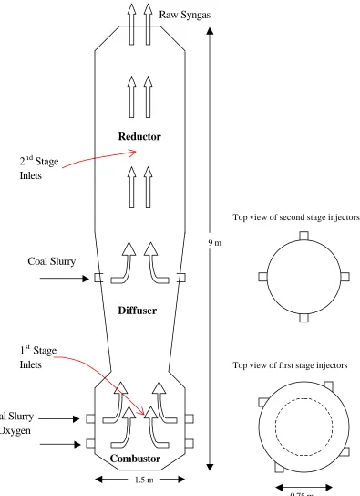
This research studies a two-stage entrained gasifiers. The geometry of the

gasifier used in the simulation is shown in Fig 2.1. The geometry and the operating

conditions are based on papers by Bockelie et al. [Bockelie et al., 2002] and by Chen et

al. [Chen et al., 1999]. The gasifier is divided into two regions: a combustion region

(combustor) in the first or the lower stage and a reduction region (reductor) in the second

or the upper stage. The gasifier has three levels of injectors that are positioned

symmetrically with two levels in the first stage, and the other is in the second stage of the

gasifier. To create swirling inside the gasifier, the lower injectors are placed similar to a

tangential firing system. . The upper injectors are aimed directly at the center of the

reductor. All oxidant and a fraction of the coal-slurry mixture are injected through the

lower injectors, and the remaining coal-slurry mixture is injected through the upper

injectors. Neither paper by Bockelie et al. [Bockelie et al., 2002] nor Chen et al. [Chen et

al., 1999] gives gasifier dimension details; therefore, some engineering judgments were

Diffuser Reductor

Combustor

1.5 m

9 m

0.75 m

Top view of second stage injectors

Top view of first stage injectors 2nd Stage

Inlets

1st Stage Inlets

Coal Slurry & Oxygen

Coal Slurry

Raw Syngas

2.1 Physical Characteristics of the Problem and Assumptions Made

The physical characteristics of the problem are as follow:

1. Three-dimensional

2. Bouyancy force considered

3. Varying fluid properties

4. Impermeable walls

The following are the general assumptions made in this study:

1. The flow is steady.

2. No-slip condition (zero velocity) is imposed on wall surfaces.

3. Chemical reaction is faster than the time scale of the turbulence eddies.

2.2 Governing Equations

The equations for conservation of mass, conservation of momentum, and energy

equation are given as:

∇⋅

( )

( )

     ⋅ ∇ + −∇ = ⋅

∇ ρ τ= ρ (2.2)

(

(

)

)

j

eff j j

eff T h J v S

p E

v _+

            _⋅ + − ∇ ⋅ ∇ = + ⋅

∇ v ρ λ

∑

where λeff is the effective conductivity (λ+λt, where λt is the turbulence conductivity) and

The stress tensor τ= is given by

(

)

vv T v

3 2

µ

τ . (2.4)

where µ is the molecular dynamic viscosity, I is the unit tensor, and the second term on

the hand side is the effect of volume dilatation. The first three terms on the

right-hand side of equation (2.3) represent heat transfer due to conduction, species diffusion,

and viscous dissipation. Sh is a source term including the enthalpy formation from the

chemical reaction of the species. The energy E is defined as

2

2

v p h

E= − +

ρ (2.5)

where h is the sensible enthalpy and for incompressible flow and is given as

ρ p h Y h j j j +

=

∑

Yj is the mass fraction of species j and

=

∫

h _, (2.7)

where Tref is 298.15 K.

2.3 Turbulence Model

The velocity field in turbulent flows always fluctuates. As a result, the

transported quantities such as momentum, energy, and species concentration fluctuate as

well. The fluctuations can be small scale and high frequency, which is computationally

computationally less expensive to solve can be obtained by replacing the instantaneous

governing equations with their time-averaged, ensemble-averaged, or otherwise

manipulated to remove the small time scales. However, the modifications of the

instantaneous governing equations introduce new unknown variables. Many turbulence

models have been developed to determine these new unknown variables in terms of

known variables. General turbulence models widely available are:

a. Spalart-Allmaras

b. k-ε models:

- Standard k-ε model

- RNG k-ε model

- Realizable k-ε model

c. k-ω model

- Standard k-ω model

- Shear-stress transport (SST) k-ω model

d. Reynolds Stress

e. Large Eddy Simulation

The standard k-ε turbulence model, which is the simplest two-equation turbulence model,

is used in this simulation due to its suitability for a wide range of wall-bound and

free-shear flows. The standard k-ε turbulence is based on the model transport equations for

the turbulence kinetic energy, k, and its dissipation rate, ε. The model transport equation

for k is derived from the exact equation; however, the model transport equation for ε is

obtained using physical reasoning and bears little resemblance to its mathematically exact

The standard k-ε turbulence model is robust, economic for computation, and

accurate for a wide range of turbulent flows. The turbulence kinetic energy, k, and its

rate of dissipations, ε, are calculated from the following equations

(

)

j k t j i i S Y G G x k x ku

x __+ + − − +

     ∂ ∂     ₊ ∂ ∂ = ∂ ∂ _ρε σ µ µ

ρ (2.8)

and

(

)

(

)

x j k b

t j i i + − + +         ∂ ∂     ₊ ∂ ∂ = ∂ ∂ 2 2 3

1 . (2.9)

In equations (2.8) and (2.9), Gk represents the generation of turbulence kinetic energy due

to the mean velocity gradients and is defined as

i j j i x u u u G ∂ ∂ − = −_ρ−−−'−'

κ . (2.10)

Gb represents the generation of turbulence kinetic energy due to buoyancy and is

calculated as i t t i b x T g G ∂ ∂ = Pr µ

β . (2.11)

Prt is the turbulent Prandtl number and gi is the component of the gravitational vector in

the i-th direction. For standard k-e model the value for Prt is set 0.85 in this study. The

coefficient of thermal expansion, β, is given as

p T

    ∂ ∂ − = ρ ρ

β 1 . (2.12)

YM represents the contribution of the fluctuating dilatation in compressible turbulence to

the overall dissipation rate, and is defined as

2

2 _t

M M

where Mt is the turbulent Mach number which is defined as

2 a

k

M = (2.14)

where a

(

)

The turbulent viscosity, µk, is calculated from equation

µ ρ µ _ε

2

k C

k = . (2.15)

The values of constants C1ε, C2ε, Cµ, σk, and σε used are

C1ε = 1.44, C2ε = 1.92, Cµ = 0.09, σk = 1.0, σε = 1.3.

The turbulence models are valid for the turbulent core flows, i.e. the flow in the

regions somewhat far from walls. The flow very near the walls is affected by the

presence of the walls. Viscous damping reduces the tangential velocity fluctuations and

the kinematic blocking reduces the normal fluctuations. The solution in the near-wall

region can be very important because the solution variables have large gradients in this

region.

However, the solution in the boundary layer is not important in this study.

Therefore, the viscous sublayer, where the solution variables change most rapidly, does

not need to be solved. Instead, wall functions, which are a collection of semi-empirical

formulas and functions, are employed to connect the viscosity-affected region between

the wall and the fully-turbulent region. The wall functions consist of:

§ laws-of-the-wall for mean velocity and temperature (or other scalars)

There are two types of wall function: (a) standard wall function and (b)

non-equilibrium wall function. The former is employed in this study. The wall function for

the momentum is expressed as

( )

U ln κ 1 _(2.16) where ρ τϖ µ 2 1 4 1 P PC k

U

U+ ≡ (2.17)

µ ρCµ kP yP

y 2 1 4 1 ≡ + _(2.18) and

κ = von Karman constant (= 0.42)

E = empirical constant (= 9.793)

UP= mean velocity of fluid at point P

kP = turbulence kinetic energy at point P

yP = distance from point P to the wall µ = dynamic viscosity of the fluid.

The wall function for the temperature is given as

(

)

( )

where P is given as

[

]

e P T P r P r 007 . 4 3 28 . 0 1 1 Pr Pr 24 .

9 + −

and

r = density of the fluid

cp = specific heat of fluid

q = wall heat flux

TP = temperature at cell adjacent to the wall

TW = temperature at the wall

Pr = molecular Prandtl number

Prt = turbulent Prandtl number (0.85 at the wall)

A = 26 (Van Driest constant)

κ = 0.4187 (von Karman constant)

E = 9.793 (wall function constant)

Uc = mean velocity magnitude at y+ = y+T

y+T = non-dimensional thermal sublayer thickness.

The species transport is assumed to behave analogously to the heat transfer. The

equation is expressed as

(

)

( )

where Yi is the local mass fraction of species i, Sc and Sct are the Schmidt numbers, and

Ji,w is the diffusion flux of species i at the wall. The turbulent Schmidt number, Sc, is

given as

D ρ

µ

, where µ is the viscosity and D is the diffusivity. The Pc and y+c are

calculated in a similar way as P and y+T, with the difference being that the Prandtl

In the k-ε model, the k equation is solved in the whole domain, including the

wall-adjacent cells. The boundary condition for k imposed at the wall is

₌₀

∂ ∂

n

k _(2.22)

where n is the local coordinate normal to the wall. The production of kinetic energy, Gk,

and its dissipation rate, ε, at the wall-adjacent cells, which are the source terms in k

equation, are computed on the basis of equilibrium hypothesis with the assumption that

the production of k and its dissipation rate assumed to be equal in the wall-adjacent

control volume. The production of k and ε is computed as

P p w w w k

y

k

C

y

U

G

κρ

τ

τ

τ

=

∂

∂

≈

ky

k

C

τ

ε

=

2.4 Radiation Model

The P-1 radiation model is used to calculate the flux of the radiation at the inside

walls of the gasifier. The 1 radiation model is the simplest case of the more general

P-N radiation model that is based on the expansion of the radiation intensity I. The P-1

model requires only a little CPU demand and can easily be applied to various

complicated geometries. It is suitable for applications where the optical thickness aL is

large where a is the absorption coefficient and L is the length scale of the domain.

4

4aG T

aG

q_r = − σ

∇

− (2.25)

where

(

)

q

s s

r =− _{+σ − σ} ∇

3

1 _(2.26)

and qr is the radiation heat flux, a is the absorption coefficient, σs is the scattering

coefficient, G is the incident radiation, C is the linear-anisotropic phase function

coefficient, and σ is the Stefan-Boltzmann constant.

The flux of the radiation, qr,w, at walls caused by incident radiation Gw is given as

(

)

(

)

where εw is the emissivity and is defined as

w

w ρ

ε =1− (2.28)

and ρw is the wall reflectivity.

2.5 Combustion Model

The global reaction mechanism is modeled to involve the following chemical

species: C, O2, N2, CO, CO2, H2O and H2 (see reactions R1.1 through R1.5 in Chapter 1).

All of the species are assumed to mix in the molecular level. The chemical reactions

inside the gasifier are modeled by calculating the transport and mixing of the chemical

species by solving the conservation equations describing convection, diffusion, and

reaction of each component species. The general form of the transport equation for each

( )

(

)

t +∇⋅ =−∇⋅ +

∂∂

r v

ρ

ρ . (2.29)

Ri is the net rate of production of species i by chemical reaction. Ji

r

is the diffusion flux

of species i, which arises due to concentration gradients. Mass diffusion for laminar flows

is given as

i m i

i D Y

Jr =−ρ _, ∇ (2.30)

For turbulent flows, mass diffusion flux is given as

_i t t m i i Y Sc D J ∇     + − = ρ , µ r (2.30

where Sct is the turbulent Schmidt number.

So, the transport equations for each chemical species are

(

)

(

)

t +∇⋅ =−∇⋅ +

∂

∂ _v r

ρ

ρ (2.32a)

( ) (

)

t +∇⋅ =−∇⋅ +

∂

∂ _v r

ρ

ρ (2.32b)

( ) (

)

t +∇⋅ =−∇⋅ +

∂

∂ _v r

ρ

ρ (2.32c)

(

)

(

)

t +∇⋅ =−∇⋅ +

∂

∂ _v r

ρ

ρ (2.32d)

(

) (

)

t +∇⋅ =−∇⋅ +

∂∂

r v

ρ

ρ (2.32e)

(

) (

)

t 2 +∇⋅ 2 =−∇⋅ 2 + 2

∂

∂ _v r

ρ

ρ (2.32f)

( ) (

)

t +∇⋅ =−∇⋅ +

∂

∂ _v r

ρ

The reaction equations that need to be solved are given below.

C(s) + ½ O2→ CO (2.33)

C(s) + CO2→ 2CO (2.34)

C(s) + H2O(g) → CO + H2 (2.38)

CO + ½ O2→ CO2 (2.36)

CO + H2O(g) → CO2 + H2 (2.37)

There are three approaches to solving these reactions.

(a) Eddy-dissipation model: The assumption in this model is that the chemical

reaction is faster than the time scale of the turbulence eddies. Thus, the reaction

rate is determined by the turbulence mixing of the species. The reaction is

assumed to occur instantaneously when the reactants meet.

(b) Equilibrium model: The rate of chemical reaction is governed by the rate of

mixing of gaseous oxidant and reactant. The reactions are fast compare to the

time scale of turbulence. The gaseous properties become functions of the

turbulent mixing rate and can be calculated using equilibrium considerations

[Fletcher, 1983].

(c) Reaction rate model: The rate of chemical reaction is computed using an

expression that takes into account temperature and pressure and ignores the

effects of the turbulent eddies.

In this study, the eddy-dissipation model is used. The sources term Ri in equation

(2.29) is calculated using the eddy-dissipation model based on the work of Magnussen

species i as the result of reaction r, Ri,r, is given by the smaller of the two expressions below.         ′ ′ = R w r R R R r i r i r i M Y k A M R , , , ,

, ν ρε min _ν (2.38)

and         ′′ ′ =

∑

∑

j jr w j P P r i r i r i M Y k B M R , , , , , ν ε ρ ν (2.39) where,

YP is the mass fraction of any product species, P

YR is the mass fraction of a particular reactant, R

A is an empirical constant equal to 4.0

B is an empirical constant equal to 0.5

v’i,r is the stoichiometric coefficient of reactant i in reaction r

v”j,r is stoichiometric coefficient of product j in reaction r.

In equations (2.12) and (2.13), the chemical reaction rate is governed by

large-eddy mixing time scale, k/ε. The smaller of the two expressions (2.12) and (2.13) is used

because it is the limiting value that determines the reaction rate.

The procedure to solve the reactions is as follows.

1. The net local production or destruction of species i in each reaction is calculated

by solving equations (2.12) and (2.13).

2. The smaller of these values is substituted into the corresponding species transport

3. Yi is then used in equation (2.11) to calculate the net enthalpy production of each

reaction equation.

4. The net enthalpy production becomes the source term in energy equation (2.3)

that affects the temperature distribution. In an endothermic process, the net

enthalpy production is negative, which becomes a sink term in the energy

equation.

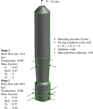
2.6 Boundary Conditions

Figure 2.3 shows the boundary conditions for the baseline case of the generic

two-stage entrained-flow gasifier. Boundary conditions for all the cases simulated in this

P = 24 atm

§ Operating pressure 24 atm.

§ No slip condition at the wall. u = 0, v = 0, w = 0

§ Adiabatic walls

§ Inlet turbulence intensity: 10%

Stage 1

Mass flow rate: 49.6 kg/s

Temperature: 425K Mass fraction:

C : 0.33 H2O : 0.29

O2 : 0.35

N2 : 0.02

Stage 2

Mass flow rate: 10.4 kg/s

Temperature: 425K Mass fraction:

C : 0.53 H2O : 0.47

O2 : 0

N2 : 0

Table 2.1 Parameters and operating conditions for simulated cases

* In Cases 6 & 7, the injectors in Stage 1 are modified to tilt 30 degrees downward (Case 6) and 30 degrees upward (Case 7).

Fuel Oxidant

Stage 1 2 Total 1 2 Total 1 2 Total

75% 25% 75% 25% 75% 25%

100% 0% 100% 0% 100% 0%

49.6 10.4 60 51.4 8.6 60 51.4 8.6 60

16.4 5.5 21.9 23.1 7.7 30.8 23.1 7.7 30.8

(kmole/s) (kmole/s) (kmole/s)

C 0.33 0.53 1.82 0.45 0.89 2.57 0.45 0.89 2.57

H₂O 0.29 0.47 1.07 0.06 0.11 0.22 0.06 0.11 0.22

O₂ 0.35 0 0.54 0.47 0 0.75 0.47 0 0.75

N₂ 0.02 0 0.04 0.02 0 0.04 0.02 0 0.04

Adia. Adia. Adia. Adia. 1800 1600

Fuel distribution

Total mass flow rate, kg/s

Wall temperature, K Oxidant distribution

Mass fraction at inlet Coal mass flow rate, kg/s

Parameters

Oxygen

Cases 1, 6 and & 7*

Oxygen Oxygen

Case 3

Coal powder

Coal slurry Coal powder

Case 2

Fuel Oxidant

Stage 1 2 Total 1 2 Total 1 2 Total

50% 50% 75% 25% 100% 0%

100% 0% 100% 0% 100% 0%

39.3 20.7 60 55 5 60 60 0 60

11.0 11.0 22.0 7.7 2.7 10.4 22.2 0.0 22.2

(kmole/s) (kmole/s) (kmole/s)

C 0.28 0.53 1.83 0.14 0.53 0.86 0.37 0 1.85

H₂O 0.25 0.47 1.09 0.13 0.47 0.53 0.32 0 1.07

O₂ 0.45 0 0.55 0.15 0 0.26 0.29 0 0.54

N₂ 0.02 0 0.03 0.58 0 1.14 0.02 0 0.04

Adia. Adia. Adia. Adia. Adia. Adia.

Case 8 Coal slurry Oxygen Air Case 5 Coal slurry Case 4 Coal slurry Parameters Oxygen Fuel distribution

Total mass flow rate, kg/s

Wall temperature, K Oxidant distribution

CHAPTER THREE

COMPUTATIONAL PROCESS

3.1 Solution Methodology

The major steps taken in performing the computational simulation are given as

follows:

1. Preprocessing:

The preprocessing phase starts with the geometry generation. This phase includes

geometry generation, mesh generation, fluid properties specifications, physical model

selection, and boundary condition specifications.

2. Processing:

In the processing phase, the equations and models set up in the preprocessing phase

are solved using the CFD code. The progress of the calculation to achieve a

converged result is observed. Sometimes adjustments on under-relaxation factors

need to be made to help reach the convergence.

3. Postprocessing:

The postprocessing phase includes the analysis and interpretation of the results. The

results can be presented in the form of x-y plots, contour plots, velocity vector plots,

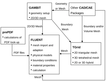
The preprocessing tool used in this study is GAMBIT, which provides one

interface to build and mesh the geometry. The CFD solver is the commercial CFD code

FLUENT Version 6.1.22. FLUENT is a finite-volume-based CFD solver written in C

language, and has the ability to solve fluid flow, heat transfer and chemical reactions in

complex geometries and supports both structured and unstructured mesh. Figure 3.1

illustrates the basic program structure that can be used to support CFD simulation in

FLUENT.

3.2 Computational Grid

The geometry is generated and meshed in GAMBIT. Three-dimensional

hexahedral mesh is used for meshing the gasifier (Figure 3.2). A total of 95,185 grids are

employed. After the model has been meshed, it is exported to FLUENT.

3.3 Numerical Procedure

The procedure for performing the simulation in FLUENT is outlined below.

1. Create and mesh the geometry model using GAMBIT

2. Import geometry into FLUENT

3. Define the solver model

4. Define the turbulence model

5. Define the species model

6. Define the materials and the chemical reactions

7. Define the boundary conditions

9. Iterate/calculate until convergence is achieved.

10. Postprocess the results

FLUENT offers two solution methods: (a) segregated solution and (b) coupled

solution. Segregated solution solves the governing equations of continuity, momentum,

energy, and species transport sequentially (segregated from one another). On the other

hand, coupled solution solves the governing equations of continuity, momentum, energy,

and species transport simultaneously. The equations for scalars such as turbulence and

radiation are solved using the previously updated values from the momentum equations.

Segregated solution is chosen for this study. The detailed steps of segregated solution are

given below.

(i) Fluid properties are updated based on the current solution or the initialized

solution.

(ii) The momentum equations are solved using the current values of pressure and

face mass fluxes to get the updated velocity field.

(iii) Equation for the pressure correction is calculated from the continuity equation

and the linearized momentum equations since the velocity field obtained in step

(ii) may not satisfy the continuity equation.

(iv) The pressure correction equations obtained from step (iii) are solved to correct

the pressure and velocity fields, and face mass such that the continuity equation

is satisfied.

(v) The equations for scalars such as turbulence, energy, radiation, and species are

(vi) The equation is checked for convergence.

These steps are repeated until the convergence criteria are met. Figure 3.3 shows the

flow chart of the above steps.

GAMBIT

•geometry setup

•2D/3D mesh

Other CAD/CAE

Packages

FLUENT

•mesh import and

adaption

•physical models

•boundary conditions

•material properties

•_calculation •postprocessing

TGrid

•2D triangular mesh

•3D tetrahedral mesh

•2D or 3D hybrid prePDF

•_{calculations of}

PDF look-up 2D/3D Mesh PDF files Mesh Mesh Boundary Mesh Boundary and/or Volume Mesh Geometry or Mesh

Update Properties

Solve momentum equations.

Solve pressure-correction (continuity) equation. Update pressure, face mass flow rate.

Solve energy, species, turbulence and other scalar equations.

Converged? Stop

No Yes

Figure 3.3 Overview of the Segregated Solution Method.

The non-linear governing equations can be linearized implicitly or explicitly with

respect to the dependent variables. If linearized implicitly, the unknown value in each

cell is computed using a relation that includes both existing and unknown values from

neighboring cells. If linearized explicitly, the unknown value in each cell is computed

using a relation that includes only existing values. In the segregated solution, the

linearization is implicit. Therefore, each unknown will appear in more than one equation

in the linear system, and these equations must be solved simultaneously to give the

unknown quantities.

FLUENT uses a control-volume-based technique to convert the governing

equations to algebraic equations, which are then solved mathematically. The

quantity on a control-volume basis. There are several discretization schemes available in

FLUENT: (a) First Order, (b) Second Order, (c) Power Law, and (d) QUICK.

The first order discretization scheme is applied for the momentum, the turbulence kinetic

energy, the turbulence kinetic dissipation, the energy, and all the species.

FLUENT provides three algorithms for pressure-velocity coupling in the

segregated solver: (a) SIMPLE, (b) SIMPLEC, and (c) PISO. The SIMPLE algorithm

[Patankar et. al, 1980] is used in this study.

The built-in standard k-ε turbulence model is used, and the model constants are as

follow: Cµ = 0.09, C1ε = 1.44, C2ε = 1.92, σk = 1.0, σε = 1.3.

FLUENT offers several species model:

• Species transport: laminar finite-rate, eddy-dissipation, or

eddy-dissipation-concept (EDC)

• Non-premixed combustion

• Premixed combustion

• Partially premixed combustion

• Composition PDF combustion

The species model and transport model with volumetric reaction are chosen to

simulate the diffusion and production/destruction of the chemical species. The

eddy-dissipation model is utilized to calculate the net production and destruction of the species.

Eddy-dissipation model assumes that chemical kinetics are fast compared to the mixing

A mixture material that consists of seven chemical species (C, O2, N2, CO, CO2,

H2O and H2) is defined. All the species, including C, are defined as fluid species and are

assumed to mix at the molecular level. The specific heat of the species is temperature

dependant and is defined as a piecewise-polynomial function of temperature. The

chemical reactions (R1.1) through (R1.5) in Chapter 1 are then defined in the reaction

window.

The types of boundary conditions on the surface geometry have been assigned in

GAMBIT. There are three types of boundary conditions for the model.

a. Mass flow rate inlet --- All the inlet surfaces are defined as mass flow rate

inlets. The mass flow rate, temperature of the mixture, and the mass fractions of

all species in the mixture are specified according to the values given in the Table

2.1 in Chapter Two.

b. Pressure outlet --- The outlet surface is assigned as a pressure outlet boundary.

The pressure, temperature, and species mass fractions of the gas mixture outside

the computational domain are specified. This information does not affect the

calculations inside the computational domain but will be used if backflow occurs

at the outlet.

c. Walls --- The outside surfaces are defined as wall boundary. The walls are

stationary with no-slip condition imposed (zero velocity) on the surface. For

adiabatic case, the heat flux on the wall is set to 0 (zero). For constant wall

temperature, the wall temperature is set to a certain constant value as specified in

The complete inlet and boundary conditions for all the cases conducted in this study are

listed in Table 2.1.

Before FLUENT can begin solving governing equations, flow field guessed initial

values, used as the initial values of the solution, have to be provided. Once the initial

values have been provided, the iteration is performed until a converged result is obtained.

An example of the step-by-step procedure for performing the baseline case is given in

Appendix A.

3.4 Grid Independence Study

A grid independence study was conducted using three different grids: coarse grid

(35,168 grids), medium grid (95,182 grids), and fine grid (160,170 grids). Parameters

and operating conditions for Case 1 given in Table 2.1 were used in this grid

independence study. The calculations were performed by a personal computer with

Pentium 4, 2.8 GHz CPU. Table 3.1 shows the mass-weighted average temperature and

species mole fractions of the exit gas for all grids. It can be seen that the exit gas

temperature for the coarse grid is the highest at 763 K followed by fine grid at 723 K and

medium grid 717 K. The temperatures for the medium and fine grids only differ by 8 K,

which is less than 1.5%. The differences in the species mole fractions for the medium

and fine grids are less than 2 percentage points, which are small and acceptable to this

study. Therefore, to ensure obtaining good results with reasonable computational time,

the medium grid is used for this study.