N. Champagnat, T. Leli`evre, A. Nouy, Editors
A FAST BOUNDARY ELEMENT METHOD FOR THE SOLUTION OF
PERIODIC MANY-INCLUSION PROBLEMS VIA HIERARCHICAL MATRIX
TECHNIQUES
∗,∗∗,∗∗∗Paul Cazeaux
1and Olivier Zahm
2Abstract. Our work is motivated by numerical homogenization of materials such as concrete, modeled as composites structured as randomly distributed inclusions imbedded in a matrix. In this paper, we propose a method for the approximation of the periodic corrector problem based on boundary integral equations. The fully populated matrices obtained by the discretization of the integral operators are successfully dealt with using theH-matrix format.
R´esum´e. Nous nous int´eressons `a l’homog´en´eisation de mat´eriaux de type b´eton, c’est `a dire com-pos´es d’agr´egats distribu´es al´eatoirement dans une matrice. Nous proposons une m´ethode pour la r´esolution du probl`eme de correcteur p´eriodique en s’appuyant sur une formulation int´egrale surfacique. Les matrices pleines obtenues par la discr´etisation des op´erateurs int´egraux sont trait´ees avec succ`es `a l’aide de matrices hi´erarchiques.
Introduction
Understanding the macroscopic properties of composite materials is of great interest in a number of industrial applications. One such example is the study of the aging of electrical nuclear plants due to the long-term behavior of concrete. Homogenization techniques have become widely used to predict this macroscopic behavior, based on the knowledge of the distribution and characteristics of the constituting elements in the microstructure of such materials. A number of different homogenization frameworks exist, ranging from qualitative methods proposed by physicists and engineering, see e.g. [21], to more rigorous mathematical methods developed for example in the periodic case [6, 29] or the stationary random case [6, 24], giving rise to a vast body of literature.
Using these techniques, the effective (macroscopic) properties of the composite are typically deduced from the solution of an elliptic boundary value problem, called corrector problem. Formulated on a representative volume element (RVE) of the microstructure, solving numerically this problem enables us to sample the local behavior of the microstructure under a macroscopic forcing. Approximate effective parameters are then obtained by averaging the computed local quantities over the RVE [6]. In the case of idealized structures such as perfect crystals, the geometry of the RVE is simple. However, in the case of composite materials such as concrete,
∗Thanks to A. Nouy, F. Legoll, Y. Assami, A. Obliger, W. Minvielle for fruitful discussions. ∗∗ The authors would like to thank the CEMRACS organizers and participants for a great stay. ∗∗∗This work was financially supported by EDF R&D.
1 MATHICSE, Chair of Computational Mathematics and Simulation Sciences, Ecole Polytechnique F´ed´erale de Lausanne,
Station 8, CH-1015 Lausanne, Szitwerland. ([email protected])
2GeM, UMR CNRS 6183, ´Ecole Centrale de Nantes, 1 rue de la No¨e, BP92101, 44321 Nantes Cedex 3, France.
c
EDP Sciences, SMAI 2015
this geometry can become quite complex. In fact, when the composite is modeled as a matrix containing a stationary random distribution of inclusions, the corrector problem is effectively set on the whole space [24]. In this case, a sequence of corrector problems is usually solved in a bounded box of increasing size. The sequence of approximate effective parameters computed in this way are known to converge to the true effective parameters as the size of the box goes to infinity [14]. Thus it is necessary to develop efficient numerical methods able to deal with complex three-dimensional geometries, induced by large numbers of inclusions in the RVE, see e.g. [9]. A number of numerical methods can be used to approach the solution of the corrector problem. A widely used approach is the direct discretization of the elliptic PDE system, either by finite differences or by the finite elements method. However, such full field simulations remain computationally limited by the large number of degrees of freedom that is required, in particular in a three dimensional setting.
We present a boundary integral reformulation of the corrector problem. We propose a numerical approach for its solution, using the boundary element method (BEM) [23], accelerated by the use of hierarchical matrices. Such methods are known to easily handle jumps in the parameters in a complicated geometry, avoid having to discretize the entire domain in a manner that accurately resolves the geometry of the inclusions, can achieve rapid convergence, and have a robust mathematical foundation [2, 23]. Specific difficulties in this framework involve in particular dealing with:
• periodic boundary conditions,
• a three-dimensional setting,
• complex geometries involving large numbers of randomly distributed inclusions in a representative pe-riodic cell.
While the overwhelming majority of works devoted to the numerical evaluation of effective properties of com-posite materials employ the finite element method [26], the BEM has been proposed in a few publications as a promising alternative to study the homogenization of composites, see e.g. [12, 16, 25]. A related investigation on periodic problems for the Stokes equation can be found in [17]. In particular, fast multipole methods have recently been designed to increase the efficiency of this approach while dealing with the periodic boundary conditions in the case of rigid inclusions for linear elasticity with applications to the homogenization of carbon nanotube materials in two or three dimensions [22, 27], based on the original fast multipole algorithms [18], see also [28].
A closely related problem is the calculation of band structure in periodic crystals or materials, to which boundary integral methods have been recently applied, see e.g. [32]. In particular, our approach is inspired by ideas proposed in [2] in a two-dimensional setting. There is also an extensive literature on the subject of integral equations for scattering from periodic structures, see e.g. [11].
The BEM discretization results in linear systems involving fully populated matrices, by contrast with the sparse systems obtained with the finite differences or finite elements methods. An algebraic tool designed to deal efficiently with such fully populated matrices is the hierarchical matrix (orH-matrix) format introduced by Hackbusch and his collaborators, see e.g. [5, 7, 19]. The main advantages of theH-matrix format are:
• the controlled approximation of the matrix with respect to a given precision,
• the reduced computational and memory cost compared to the usual matrix storage,
• and the accelerated algebraic operations (matrix-vector product, linear solvers,etc).
1.
The periodic corrector problem
1.1.
Reformulation of the corrector problem as a boundary integral problem
In this section we derive a boundary integral formulation for the corrector problem associated to the Laplace equation. Let Ω = (−1/2,1/2)d be an open unit periodic cell in
Rd,d= 2,3. We decompose Ω as a set of closed
inclusions Ωint ⊂Ω and a connected matrix Ωext = Ω\Ωint, see figure 1. In the following, Γ =∂Ωint denotes
the boundary of the set of inclusions.
Figure 1. Example of the geometry of a set of inclusions.
Remark 1.1. It is not necessary to suppose that the inclusions are distributed strictly inside the periodic cell. Let κ(x) be a scalar diffusion coefficient which takes two different values κint,κext >0 respectively in the
inclusions and in the matrix:
κ(x) = (
κint in Ωint,
κext in Ωext.
(1)
We are interested in the periodic correctoru∈H1(Ω)/Rsolution of the following boundary value problem:
(
−div(κ(E+∇u)) = 0, in Ω,
uis Ω-periodic, (2)
where E∈R3 is a given macroscopic gradient of some diffusive quantity
e
u. The problem (2) is the system of equilibrium equations on the RVE for the Laplace equation, assuming that the real gradient is split into two parts as
∇ue=E+∇u,
where Eis the overall gradient and∇uthe fluctuating terms. It is well–known that problem (2) has a unique solution, see e.g. [1]. Note that the solutionuis harmonic in Ω\Γ and satisfies continuity conditions:
u, κ(∇u+E)·nextcontinuous across Γ, (3) where next is the exterior normal to Γ. An elegant approach for the integral representation of periodic fields
delta function centered at the origin. The periodic Green’s functionGperis then defined by−∆Gper=δ0−1 over
Ω (note that the right-hand side must have zero mean over the periodic cell). Let us introduce the single-layer potential [23] as an operatorH−1/2(Γ)→H1(Ω) defined by:
(ΨSLσ)(x) =
Z
Γ
Gper(x−y)σ(y)ds(y) forx∈Ω\Γ. (4)
We can represent the solution to the PDE problem (2) asu= ΨSLσ with a single-layer densityσ. It remains
to solve for the density σ∈H−1/2(Γ) so that the matching conditions (3) are satisfied. We use the standard
jump relations for single layer potential [23] to write
κext(−1/2Id+K00)σ−κint(1/2Id+K00)σ=−(κext−κint)E·next on Γ, (5)
where Idis the identity operator andK00 is the adjoint double layer boundary integral operatorH−1/2(Γ)→ H1/2(Γ) formally defined as:
(K00σ)(x) = Z
Γ
σ(y)∇xGper(x−y)·next(y)ds(y). (6)
Finally, we obtain the following boundary integral equation:
κ
ext+κint κext−κint
Id−K00
σ=E·next, (7)
where the operator appearing on the left–hand side is a compact perturbation of the identity.
1.2.
Approximation of the periodic Green’s function
A Galerkin approach is used to discretize (7) given a mesh of the boundary Γ. Functions in H−1/2(Γ) are
approximated by constant-by-cell functions. The main difficulty is the computation of values of the periodic Green’s function necessary to the discretization of the boundary integral operator K00 defined by (6). Indeed, while the free–space Green’s function is given by an analytical expression, the periodic Green’s function is not known explicitely. It is rather given by a Fourier series,
Gper(x) =
X
k∈Zd; k6=0
e2iπk·x
|k|2 .
Because such sums converge too slowly to be numerically useful, a number of schemes have been devised for their evaluation, see e.g. [8, 13]. We use here a different, new approach, based on an idea proposed recently by Barnett and Greengard [2] for the Helmholtz two–dimensional case. Observe that the periodic Green’s function can be represented in Ω as
Gper(x) =G∞(x) + |x|2
6 +G
r
per(x), (8)
whereG∞is the free-space Green’s function (satisfying−∆G∞=δ0 over the whole domainRd), andGrper, the
”regular” part of the periodic Green’s function, is a smooth, harmonic function in Ω. It can thus be expanded on the basis of the solid spherical harmonics as a series converging uniformly in Ω:
Grper(x) = ∞
X
l=0 l
X
m=−l αml Φ
m
where Φm
l is the regular solid harmonics of degree l and order m and the α m
l are scalar coefficients. An
approximation toGr
per can then be computed by truncating the expression (9) up to some degreeL∈N, given
that we tabulate beforehand the coefficients of the expansionαm
l forl≤L.
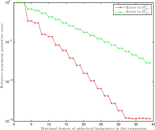
0 5 10 15 20 25 30 35 40
10−15 10−10 10−5 100 R e la t iv e m a x im u m p o in t w is e e r r o r
M a x i m a l d e g r e e o f s p h e r i c a l h a r m o n i c s i n t h e e x p a n s i o n E r r o r t oGgr
p e r E r r o r t oGr
p e r
Figure 2. Convergence in pointwise error, sampled in Ω, for the periodic Green’s function scheme.
To achieve this, we construct a small linear system that enables us to compute an approximation to the coefficientsαm
l easily, as in [2], paragraph 3.2. The general idea is to enforce numerically the periodic boundary
conditions on the approximation toGper based on the representation (8) and (9). In practice, we use a least–
squares algorithm, minimizing the L2-norm of the deviation from periodicity of the function and its normal
derivative on ∂Ω, sampled at Gaussian quadrature points. We refer to the forthcoming paper [10] for a more complete description and analysis of this method.
This method, implemented in Matlab, allows us to achieve an exponential convergence rate as shown by the green curve in figure 2. It can be further accelerated by removing from the regular part Gr
per copies of the
free-space Green’s function centered in the nearest neighbor cells. We then compute and use the coefficientsβlm
in the following expansion:
] Gr
per(x) = ∞
X
l=0 l
X
m=−l
βlmΦml (x) =Gper(x)−
X
m∈{−1,0,1}3
G∞ x+
3
X
i=1 miei
!
−|x| 2
6 , (10)
where the ei are the vectors of the standard basis ofR3. The convergence rate is much improved as seen in
figure 2. Note that, due to the symmetry of the square unit cell, only harmonics of even degreel≥4 and order
m multiple of 4 have a nonzero coefficientβm
l in (10). We use this approximation below, fixingL= 8, which
ensures a relative error in the computation of the corrective termG]r
per of about 10−4.
reduce the complexity of the computation, compression techniques such as multipole expansions (e.g. the fast multipole method) or hierarchical matrices can be used; in this paper, this latter approach is investigated (see section 2).
Remark 1.2. Since the goal of this study is to explore the use of the hierarchical matrix format in the context of the solution of the corrector problem, we do not fully detail here the numerical discretization method which is quite standard, see e.g. [30] and we refer to a forthcoming paper [10] for the full description of the approach. We limit ourselves to the case of a smooth boundary Γ in dimension d= 3.
2.
H
-matrix
In this section we recall the main properties of the hierarchical matrix format, also calledH-matrix. This format, first introduced by Hackbusch in [19], is an algebraic tool designed mainly to manage large linear systems with fully populated matrices. For a more in-depth description, we refer to [5, 7]. This format as two main advantages for numerical computation:
• it provides a controlled approximation of the matrix that reduces the memory requirements,
• all algebraic operations (matrix-vector product, LU-factorization, etc) can be accelerated compared to the full storage.
2.1.
Motivations
The H-matrix format can be introduced as a data-sparse approximation of matrices resulting from the discretization of non local integral operators [20] of type:
Z
Ω
g(x,y)u(y)dy=f(x), ∀x∈Ω, (11)
where the kernelg (possibly singular) is assumed to be asymptotically smooth, that is to satisfy :
|∂xα∂yβg(x,y)| ≤C1(C2kx−yk)−|α|−|β||g(x,y)|, C1, C2∈R withα, β∈Nd. (12)
In the present paper, the considered integral equation is the boundary integral equation (7). We look for the weak solutionu∈V (withV an appropriate Hilbert space) of problem (11) which satisfiesa(u, v) =b(v) for all
v∈V, where a(·,·) andb(·) are defined by :
a(u, v) = Z
Ω
Z
Ω
g(x,y)v(x)u(y)dydx, b(v) =
Z
Ω
f(x)v(x)dx.
Under classical assumptions on the kernel g(·,·), the bilinear form ais coercive and (by the Lax-Milgram lemma) the variational problem is well posed [20]. The Galerkin approximationuhon a finite element subspace
Vh = span{φi}1≤i≤n (φi being shape functions with compact, localized support) is defined by the relation uh=Pn
i=1Uiφi, where the coefficients{Ui}1≤i≤n are the solution of the linear system
AU =B, (13)
withAi,j =a(φi, φj) andBi=b(φi).
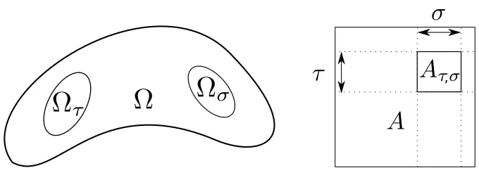
In order to motivate the following, let us consider two subsets of indices τ, σ ⊂ {1, . . . , n}, and Ωτ = ∪i∈τsupp(φi) and Ωσ=∪i∈σsupp(φi) two clusters of Ω such that :
withη >0. This last condition is called theadmissibility condition.
,
Figure 3. Representation of two admissible clusters Ωτ and Ωσ (left) and the corresponding
block in the matrixA(right).
In such a situation (see figure 3), the restriction of the kernelgon Ωτ×Ωσ usually has a low rank structure:
for anyε >0 there exists k∈N, depending on εand relatively small [15], and there exists pairs of functions
(h1l, h2l)∈L2(Ωτ)×L2(Ωσ) withl ∈ {1, . . . , k} such that the sumge(x,y) =P k l=1h
1 l(x)h
2
l(y), called ak-rank
function, is such that:
kg(x,y)−eg(x,y)kL2(Ωτ×Ωσ)≤εkg(x,y)kL2(Ωτ×Ωσ). (15)
For example,egcan be expressed e.g. with a truncated Taylor series or an interpolation scheme, see [5,7]. The existence of such a low rank approximation ensures that the block Aτ,σ also has a low rank structure. Indeed,
replacingg byegin the definition of the blockAτ,σ, we obtain:
(Aτ,σ)i,j≈
Z
Ω
Z
Ωe
g(x,y)φσ(j)(x)φτ(i)(y)dydx
=
k
X
n=1
Z
Ω
h1n(x)φσ(j)(x)dx
| {z }
Bi,k
Z
Ω
h2n(y)φτ(i)(y)dy
| {z }
Cj,k
= (BCt)i,j.
Thus, for anyε >0 there existsB∈R|σ|,k andC∈R|τ|,k withksmall (i.e. k |σ|andk |τ|) such that:
kAτ,σ−BCtkF ≤εkAτ,σkF, (16)
where k · kF denotes the Frobenius norm, and we denote by | · |the cardinal of a set of indices. The storage
requirement of the approximation isk(|τ|+|σ|), which is significantly lower than the|τ|.|σ|needed for the full storage ofAτ,σ.
TheH-matrix format relies on:
• a block partition of the matrix that contains blocks satisfying the admissibility condition (14),
• a low-rank approximation of those admissible blocks with respect to a given precision (16).
In the following, we present the classical procedure for the approximation of an integral operator in theH-matrix format [5].
2.2.
Cluster tree and block tree partition
TI ofI, defined in the following paragraph. Each node of that tree is a set of indicesσ⊂I that corresponds
to a subdomain Ωσ =∪i∈σsupp(φi) of Ω, so thatTI equivalently define a partition tree of Ω. The creation of TI is so that the partition of Ω contains a large number of subdomains that are potentially admissible. The
second step is the detection of admissible blocks : if σ, τ ∈ TI are so that Ωσ and Ωτ satisfy (14), then those
indices corresponds to a block ofA. In practice, the detection of admissible blocks is done recursively in order to optimize the block partition of A. It results in a block tree partition presented in the next paragraph.
Remark 2.1. Only geometrical information is needed for the creation of the block partition.
Cluster tree partition.A treeTI, with nodesTI, is called a cluster tree if the following conditions hold :
(1) TI ⊂ P(I)\{∅}, i.e. each node ofTI is a subset of the index setI,
(2) I is the root ofTI,
(3) Ifτ∈TI is a leaf, then|τ| ≤Cleaf, i.e. the leaves consist of a relatively small number of indices,
(4) Ifτ∈TI is not a leaf, then it has two sons and their union is disjoint.
The cluster tree TI is recursively constructed with a functionsplit. Starting from the root τ =I and from
an initial treeTI that contains only the rootI, the algorithm proceeds as follow :
procedure TI =build cluster tree(τ,TI):
if|τ| ≥Cleaf,
[τ1, τ2] = split(τ),
addτ1,and τ2 inTI as sons ofτ,
callTI =build cluster tree(τ1,TI),
callTI =build cluster tree(τ2,TI),
end.
Remark 2.2. The valueCleaf = 15 classically leads to optimal computation time [5].
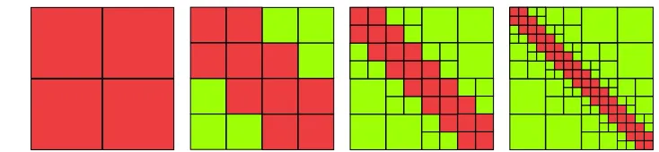
Note that the function [τ1, τ2] = split(τ) typically uses geometrical information to split the node τ. For
each index i∈τ, let xi be the center of the support ofφi. For example, a well balanced tree can be obtained
with a geometric bisection on the collection of pointsxi, meaning that ifxi is on one side of the corresponding
hyperplane,iwill be assigned inτ1; otherwise inτ2. In figure 4 we illustrate the algorithm for the construction
of the cluster tree partition.
Figure 4. Construction of the cluster partitioning of Ω
Block tree partition. Given a cluster tree partitionTI, the block tree partitionBI,IofAis a tree that contains
at each node a pair (τ, σ) of indices ofTI. The leaves ofBI,I corresponds to admissible blocks (14). It can be
constructed by the following procedure (see figure 5) initialized with τ =σ =I and BI,I the block tree that
contains only the root (I, I):
procedure BI,I =build block tree(τ, σ,BI,I)
if (τ, σ) is not admissible, and|τ| ≥Cleaf, and|σ| ≥Cleaf S={(τ∗, σ∗), τ∗ son ofτ, σ∗ son ofσ},
addS in BI,I as son of (τ, σ),
BI,I =build block tree(τ∗, σ∗,BI,I)
end for end.
Figure 5. Construction of the block tree partition at level 1,2,3,4 of call of thebuild block tree
function. The green blocks are admissible : at the end, only blocks of size < Cleaf are not
admissible (pink). This matrix corresponds to a discretized 1D Laplace operator.
The complexity of algorithms for the creation of suitable cluster trees and block tree partitions has been analyzed in detail in [15]. For typical quasi-uniform grids, a “good” cluster tree can be created in O(nlogn) operations, the computation of the block partition can be accomplished inO(n) operations.
2.3.
Approximation of the blocks
We continue this presentation by giving here some details on the construction of a low-rank approximation of each matrix block Aτ,σ. The truncated singular value decomposition (SVD) is the optimal decomposition
meaning that the relative precision ε of (16) is archieved with minimal rank kτ,σ. But the SVD procedure
requires the knowledge of the entire blockAτ,σ.
To reduce the computational cost, the adaptive cross approximation (ACA) algorithm constructs a low rank approximation based on the knowledge of only a few particular rows and lines of the block. A first method for choosing these rows and lines, called ACA with full pivoting, has been proposed in [31]. In particular, it results in a quasi-optimal approximation. The drawback of this algorithm is that the determination of the ideal pivot requires the knowledge of the entire block, as described in the next paragraph. In [3] the authors proposed a different algorithm, called ACA with partial pivoting. In this case, the choice of the pivot is made in such a way that fewer block entries are needed.
ACA with full pivoting.We consider a n-by-m matrix M. The adaptive cross approximation is a greedy procedure on the approximationMk=Pk
ν=1a
ν⊗bν ofM. Each iteration consists in the following steps :
(1) Find the pivot (i∗, j∗) such that :
(i∗, j∗) = arg max
ij |Mij−M k
ij| (17)
(2) Compute the two vectorsaki = (Mij∗−Mijk∗)/(Mi∗j∗−Mik∗j∗) andbkj = (Mi∗j−Mik∗j)
(3) Update the approximationMk+1=Mk+ak⊗bk.
The iterations are stopped when the desired precision is achieved using the condition (16).
In the general case there is no result on the rate of convergence. But when the matrix corresponds to a block of an discretized integral operator with asymptotically smooth the kernel g, it is proved that the convergence is exponential [5]. Moreover, this approximation is quasi-optimal. However the first step is to find the largest matrix entry (full pivoting (17)), which, as for the SVD, requires the knowledge of the full matrixM. The ACA algorithm with partial pivoting uses a different approach for the selection of the pivot (i∗, j∗) which enables a
ACA with partial pivoting.The idea of partial pivoting is to maximise|Mij−Mijk|only for one of the two
indices i or j and keep the other one fixed, i.e., we determine the maximal element in modulus in one particular row or one particular column. The new pivoting strategy consists at each iteration in:
(1) For a given indexi∗, find the indexj∗ such that :
j∗= arg max
j |Mi
∗j−Mik∗j| (18)
(2) Compute the two vectorsaki = (Mij∗−Mijk∗)/(Mi∗j∗−Mik∗j∗) andbkj = (Mi∗j−Mik∗j)
(3) Update the approximationMk+1=Mk+ak⊗bk, (4) Find the indexi∗ such that :
i∗= arg max
i |Mij
∗−Mijk∗|= arg max i |b
k
j| (19)
The stopping criterion (16) is replaced by a stagnation-based error estimator:
kak⊗bkkF ≤εkMkkF. (20)
The particularity of this algorithm is that we do not have to compute all matrix entries ofM. On the other hand, convergence is not guaranteed: one can find in [7] several counterexamples where ACA with partial pivoting is unable to reach the desired precision (16). Note that there exists a number of variants of this algorithm, such as the improved ACA and the Hybrid Cross Approximation [5, 7]: using additional heuristics, they try to improve on some typical failures of the basic ACA algorithm.
3.
Numerical results
3.1.
Implementation
We present here some numerical results to illustrate the proposed method for the resolution of the corrector problem. For the implementation, we used the open-source boundary element library BEM++ [30] interfaced with the library Ahmed [4] for an efficient representation of the discretized integral operators by H-matrices. All timings are reported for a laptop running the Python / C++ code with a 2.7 GHz Intel Core i7 CPU. Three different microstructures are studied containing respectively 42, 98 and 203 randomly distributed inclusions, with nine different meshes ranging from 1344 to 89140 elements. The diffusion coefficient κtakes the value 1 in the matrix and 100 in the inclusions. The precision used for theH-matrix compression with ACA algorithm (see section 2) is set toε= 1e−3.
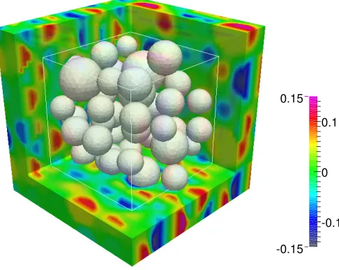
Some graphical representations of the solution are shown in figure 6. In particular, we can observe the perturbation on the corrector field induced by the periodic copies of the inclusions where the diffusion coefficient is much higher than in the matrix.
3.2.
Analysis of the
H
-matrix approximation efficiency
We finally investigate here the scalability of the boundary element approach presented above. As a bench-mark, we will also include results obtained with the same data, but replacing the periodic by the free-space Green’s function. The behavior and scaling of the method with the number of degrees of freedom is well-known in this case, see e.g. [30].
We present in table 1 some data collected during the calculations. We observe that the memory storage for the
-0.1 0 0.1
-0.15 0.15
(a)Microstructure with 42 inclusions (meshed with 18424 triangles)
-0.1 0 0.1
-0.15 0.15
(b)Microstructure with 98 inclusions (43034 triangles)
-0.1 0 0.1
-0.15 0.15
(c)Microstructure with 203 inclusion (89140 triangles)
Figure 6. Representation of the reconstructed field of the correctoru, computed by the
bound-ary element method for the three studied microstructures.
the much higher cost of evaluation of the periodic Green’s function using the representation (8), by a factor of about 50.
While no specific optimization effort has been made in the implementation of the periodic Green’s function using formula (10), let us stress that a large part of the additional computational cost is due to the direct summation over the 27 free-space Green’s function centered in the neighboring cells. In fact, due to the symmetry of the unit cell, only harmonics of even degree l ≥ 4 and order m multiple of 4 have a nonzero coefficient βm
l in (10) thus already limiting the impact of their (relatively expensive) evaluation in the total
mesh size Case storage compression ACA time solver 44784 triangles Free-space 615 Mb / 15301 MB 4.02% 63s 76s 44784 triangles Periodic 1012 Mb / 15301 MB 6.6% 3146s 118s 89140 triangles Free-space 1374 MB / 60622 MB 2.26% 128s 190s 89140 triangles Periodic 2210 MB / 60622 MB 3.6% 6402s 288s
Table 1. Data for the solution of the boundary element problem in a geometry with 203 inclusions
tabulated values of the periodic Green’s function, precomputed using (10) and using the symmetry of the cell to reduce the memory requirements.
Figure 7 illustrates however that the scaling in performance with problem size is independent of the kernel and also of the number of inclusions in the computational geometry: in all cases we observe a memory and time cost scaling approximately asO(N1.3).
103 104 105
100
101
102
103
104
Number of triangles in the mesh
Time
(s)
free-space case periodic case
(a)Assembly time for the discrete operator
103 104 105
100
101
102
103
104
Number of triangles in the mesh
Memory
(MB)
free-space case periodic case
(b)Storage for the discrete operator
Figure 7. Computational cost scaling as a function of mesh size for the periodic and the
free-space cases.
4.
Conclusion
We have proposed a new approach to the solution of the corrector problem by the use of boundary integral equations. The periodic boundary conditions are ensured through an approximation of the periodic Green’s function. Then, theH-matrix technique has been successfully applied for the resolution of the fully populated linear system araising from the Galerkin approximation of the corresponding boundary integral equation. The gain of memory and of computational costs provided by the H-matrix format has allowed to deal with a very large number of degrees of freedom in the simulation. The first results are very promising, and we hope to further develop this method which will be presented in details and compared to existing approaches in [10].
References
[1] G. Allaire. Homogenization and two–scale convergence.SIAM J. Math. Anal., 23(6):1482–1518, 1992.
[2] A. Barnett and L. Greengard. A new integral representation for quasi-periodic fields and its application to two-dimensional band structure calculations.Journal of Computational Physics, 229(19):6898 – 6914, 2010.
[4] M. Bebendorf. Another software library on Hierarchical Matrices for elliptic differential equations (AHMED). Universit¨at Leipzig, Fakult¨at f¨ur Mathematik und Informatik, 2005.
[5] M. Bebendorf.Hierarchical matrices: a means to efficiently solve elliptic boundary value problems, volume 63 ofLecture Notes in Computational Science and Engineering. Springer, 2008.
[6] A. Bensoussan, J.-L. Lions, and G. Papanicolaou.Asymptotic analysis for periodic structures, volume 5 ofStudies in Mathe-matics and its Applications. North-Holland Publishing Co., Amsterdam, 1978.
[7] S. B¨orm, L. Grasedyck, and W. Hackbusch. Hierarchical matrices. Lecture notes, Max Planck Institut f¨ur Mathematik, 2004. [8] J. M. Borwein, M. L. Glasser, R. C. McPhedran, J.G. Wan, and I. J. Zucker.Lattice Sums Then and Now, volume 150 of
Encyclopedia of Mathematics and its Applications. Cambridge University Press, 2013.
[9] S. Brisard.Analyse morphologique et homog´en´eisation num´erique, application `a la pˆate du ciment. PhD thesis, Universit´e Paris-Est, 2011.
[10] P. Cazeaux and O. Zahm. Solving three-dimensional corrector problems in random homogenization with the boundary element method. in preparation, 2014.
[11] W. C. Chew, J. M. Jin, E. Michielssen, and J. Song.Fast and Efficient Algorithms in Computational Electromagnetics. Artech House, Boston, MA, 2001.
[12] J. W. Eischen and S. Torquato. Determining elastic behavior of composites by the boundary element method. Journal of applied physics, 74(1):159–170, 1993.
[13] P.P. Ewald. Die Berechnung optischer und elektrostatischer Gitterpotentiale.Ann. Physik., 369(3):253–287, 1921.
[14] A. Gloria and F. Otto. An optimal error estimate in stochastic homogenization of discrete elliptic equations.The Annals of Applied Probability, 22(1):1–28, 2012.
[15] L. Grasedyck.Theorie und Anwendungen Hierarchischer Matrizen. PhD thesis, University of Kiel, 2001.
[16] L. Greengard and J. Helsing. On the numerical evaluation of elastostatic fields in locally isotropic two-dimensional composites.
Journal of the Mechanics and Physics of Solids, 46(8):1441–1462, 1998.
[17] L. Greengard and M. C. Kropinski. Integral equation methods for stokes flow in doubly-periodic domains.Journal of engineering mathematics, 48(2):157–170, 2004.
[18] L. Greengard and V. Rokhlin. A fast algorithm for particle simulations.Journal of computational physics, 73(2):325–348, 1987. [19] W. Hackbusch. A Sparse Matrix Arithmetic Based on H-Matrices. Part I: Introduction to H-Matrices.Computing, 62(2):89–108,
1999.
[20] W. Hackbusch and L. Grasedyck. An introduction to hierarchical matrices.Mathematica Bohemica, 127(2):229–241, 2002. [21] Z. Hashin and S. Shtrikman. A variational approach to the theory of the elastic behaviour of multiphase materials.Journal of
the Mechanics and Physics of Solids, 11(2):127–140, 1963.
[22] K Houzaki, N. Nishimura, and Y. Otani. An fmm for periodic rigid-inclusion problems and its application to homogenisation.
Contemporary mathematics, 408:81–98, 2006.
[23] G. C. Hsiao and W. L. Wendland.Boundary integral equations, volume 164 ofApplied Mathematical Sciences. Springer-Verlag, Berlin, 2008.
[24] S.M. Kozlov. Averaging of random operators.Mathematics of the USSR-Sbornik, 37(2):167, 1980.
[25] Y. J. Liu, S. Mukherjee, N. Nishimura, M. Schanz, W. Ye, A. Sutradhar, E. Pan, N. A. Dumont, A. Frangi, and A. Saez. Recent advances and emerging applications of the boundary element method.Applied Mechanics Review, 64(3), 2011. [26] V. P. Nguyen, M. Stroeven, and L. J. Sluys. Multiscale continuous and discontinuous modeling of heterogeneous materials: a
review on recent developments.Journal of Multiscale Modelling, 3(4):1–42, 2011.
[27] Y. Otani and N. Nishimura. A fast multipole boundary integral equation method for periodic boundary value problems in three-dimensional elastostatics and its application to homogenization. International Journal for Multiscale Computational Engineering, 4(4), 2006.
[28] G. J. Rodin and J. R. Overfelt. Periodic conduction problems: the fast multipole method and convergence of integral equations and lattice sums.Proceedings of the Royal Society of London. Series A: Mathematical, Physical and Engineering Sciences, 460(2050):2883–2902, 2004.
[29] E. Sanchez-Palencia. Homogenization in mechanics. a survey of solved and open problems.Rend. Sem. Mat. Univers. Politecn. Torino, 44(1), 1986.
[30] W. Smigaj, S. Arridge, T. Betcke, J. Phillips, and M. Schweiger. Solving Boundary Integral Problems with BEM ++.preprint, 2012.
[31] E. E. Tyrtyshnikov. Incomplete cross approximation in the mosaic–skeleton method.Computing, 64(4):367–380, 2000. [32] J. Yuan, Y. Y. Lu, and X. Antoine. Modeling photonic crystals by boundary integral equations and Dirichlet-to-Neumann