FORECASTING FUTURE DATA OF WHEAT AND PADDY PRODUCTION OF PUNJAB BASED ON ERROR ESTIMATION

1 | P a g e

FORECASTING FUTURE DATA OF WHEAT AND

PADDY PRODUCTION OF PUNJAB BASED ON

ERROR ESTIMATION

Dr Madhuchanda Rakshit

, Sukhpal Kaur

Applied Science Department , College of Engineering and Technology , Guru Kashi University

Talwandi Sabo , Bathinda, Punjab (India)

Research Scholar ,Guru Kashi University , Talwandi Sabo , Bathinda, Punjab (India)

ABSTRACT

This study evaluated measures for making comparisons of errors using time series. Many measures of forecast accuracy have been proposed in the past, and several authors have made recommendations about what should be used when comparing the accuracy of forecast methods applied to time series data. . In this paper statistical time series modelling techniques like moving average and least square method are used to study the future requirement of paddy and wheat and their performances are evaluated in terms of Mean absolute error (MAE), Mean square error (MSE) and Mean absolute percentage error(MAPE).

Keywords

-

Least square method, Mean absolute error (MAE), Mean Square error (MSE) , Mean

absolute percentage error (MAPE)and Moving average method

I. INTRODUCTION

Forecasts of agricultural production and prices are intended to be useful for farmers, governments, and agribusiness industries. Because of the special position of food production in a nation‟s security, governments have become both principal suppliers and main users of agricultural forecasts. They need internal forecasts to execute policies that provide technical and marketing support for the agricultural sector.

Generally forecasting techniques used past or historical data in the form of time series. A time series can be defined as an ordered sequence of random variables over time . It is the historical record of any activity , with observation taken at equally spaced intervals. Many measures on forecast accuracy have been proposed in the past, and several authors have made recommendations about what should be used when comparing the accuracy of forecast methods applied to univariate time series data. It is our contention that many of these proposed measures of forecast accuracy are not generally applicable in reality are found infinite or undefined, and can produce misleading results. The authors like Brockwell and Davis [2],[4] and Michael Lawrence[9] et al. Recently provides a new series of work on time series forecasting. In this paper, we provide our own recommendations of forecasting future data of paddy and wheat production of Punjab, India and provide the future demand of this product and also provide an empirical comparison.

2 | P a g e

environmentally and economically sustainable farming. Recently Becker Reshef et al.[ 15] and later S. Skakun et. al.[3],[15] provided a detail study of wheat production and its forecasting values[11],[16].

Over the past-two decades, many studies have been conducted to identify the appropriate method for finding the most accurate forecasts for a given class of time series. Such generalizations are important because organizations often rely upon a single method for data. Thus, it is particularly a problem when trying to specify the best method for a well-defined set of conditions, Thus it is important to identify which error measures are useful under given series. Thus error measures play an important role in refining a time series model such that it will be an accurate forecasting error for a given set of data.

Various time series models were developed by many authors for average yield for the concerned study area. Moving average method is the most used historical method for forecasting future data. Moving averages are developed at an average of weighted observations, which tends to smooth out short-term irregularity in the data series. Moving Average method has the great merit of flexibility involving construction by taking averages of several sequential values of another time series[10]. It is a type of mathematical convolution. The greater number of periods in the moving average the greater the smoothing effect. In this regard the authors like Robert, .J Hatchett [13 ] and Rob, J. Hyndman [14 ],[19] has done an influential work recently.

The least square method is a mathematical optimization technique, which is used to infer the best function matching relationship between the discrete data by the square of the difference between the measured value and the actual value[6],[7] . In engineering technology and scientific experiment, the data set is often obtained. Determining the appropriate function curve according to the data is the main problem of curve fitting in experimental data processing. Curve fitting method is the most commonly used methods and the fitting of the piecewise curve is better than the general curve fitting effect . In this regard a lot of work has already been done. So far, a lot of practical curve fitting methods have been put forward.

Error measurement statistics play a critical role in tracking forecast accuracy, monitoring for exceptions, and benchmarking your forecasting process[8],[12]. Interpretation of these statistics can be tricky, particularly when working with low-volume data or when trying to assess accuracy across multiple items[1] . Many measures of forecast accuracy have been proposed in the past, and several authors have made recommendations about what should be used when comparing the accuracy of forecast methods applied to time series data[5]. Although various stochastic and deterministic measures are available in the literature to evaluate the performance of forecasting techniques, in this paper the MSE, MAE and MAPE are used for our convenience[18],[20]. The main emphasis of this work is to compare the various forecasting techniques[8]. In this manuscript an attempt also has been made to forecast the production by using the Moving Average Method and Least Square Method. The aim is to evaluate the performances in terms of MAE,MSE and MAPE. Finally, we compare the findings and decide the suitability among the methods MAE, MSE and MAPE and also with the classic methods like MA and Least square method.

In this paper, a procedure for applying time series analysis to forecast production is described. The moving average and least square method are applied to our given set of data based on the production of wheat and paddy of Punjab. Our study is mainly based on the deterministic measures like Mean absolute error (MAE), Mean square error (MSE) and Mean absolute percentage error(MAPE).

3 | P a g e

the obtained results of the least square method are provided elaborately. Next, in section 5 and 6 detailed discussion of results are discussed and finally a conclusion is given regarding forecasting procedure.

II. METHODOLOGY

A moving average is a technique to get an overall idea of the trends in a data set; it is an average of any subset of numbers. The moving average is extremely useful for forecasting long-term trends. We can calculate it for any period of time. The formula for moving average is

Where = Forecast for the coming period , n= Number of period to be averaged

In the past period, two or three periods ago and so on respectively .Equal weighting is given to each of the values used in the moving average calculation. Whereas it is reasonable to suppose that the most recent data is more relevant to current conditions .The moving average calculation takes no account of data outside the period of average, so full use is not made of all the data available.

Least squares method is one of the statistical methods used to find out the line of best fit for a model where the line of best fit is such that it minimizes the sum of squares of the distances of the points from this line. The points represent observed data values whereas the best fit line will give a statistical model for the process. The formula for least square method is

= a+bx

Where = commuted value of the trend , x = independent variable which represents time , a=Value of trend when x is zero (y intercept) , b= slope of the line. Here „a‟ and „b‟ are constants .Once their values are determined they do not change. The value of „b‟ represents the amount by which the trend increases or decreases for each unit of time. The values of „a‟ and „b‟ are computed by solving a set of simultaneous equations,

commonly called normal equations Normal equations are:

In above equations, y represents original values in a time series, N stands for the number of years and x represents time.

There are many ways to measure forecast accuracy. Some of these measures are the mean absolute error (MAE), mean square error (MSE) and the mean absolute percentage error (MAPE). These error estimates helps in monitoring erratic demand observations. In addition they also help to determine when the forecasting method or no longer tracking actual demand and it need to be reset. The mathematical formulas

Error= Actual value- Forecast value

Mean absolute error =

Mean Square error =

Mean absolute percentage error =

4 | P a g e

In this study we used the data of wheat and paddy production for the period 2005-06 to 2016-17.Data obtained from Punjab Mandi Board, Mohali, Chandigarh. Moving average and Least square methods are applied and their performance evaluated in terms MAE,MSE and MAPE.

Table(1):Recorded wheat and paddy production data of Punjab Mandi Board , Mohali , Chandigarh

S.NO.

YEAR

PADDY(In lakh tones)

WHEAT(In lakh tones)

1

2005-06

25.18

10.53

2

2006-07

28.61

10.52

3

2007-08

26.42

12.6

4

2008-09

36.01

18.4

5

2009-10

41.31

16.69

6

2010-11

40.7

16.95

7

2011-12

33.54

17.51

8

2012-13

37.92

22.08

9

2013-14

37.12

20.24

10

2014-15

36.8

22.07

11

2015-16

35.6

15.9

12

2016-17

36.5

18.95

IV. RESULT ANALYSIS

In this section, we used the data for wheat and paddy production for the period 2005 to 2016-17. The various methods are applied one by one and their performances are evaluated in terms of MAE, MAPE and MSE.

4.1 Moving Average Method

In this section at first we obtain the Moving average results by taking 3 types of data span. Table 2 shows actual and estimated values of paddy production by 3 yearly , 5 yearly and 7 yearly moving average. The figure 1 shows the same results graphically for better understanding of the smoothness of the data. Similarly Table 3 and figure 2 shows the result of moving average by taking the same length of year for wheat production and also provide its smoothness based on moving averages.

5 | P a g e

6 | P a g e

4.2

Evaluating the Forecast Accuracy based on Moving Average

7 | P a g e

convenient to use the function itself. This is called the mean square error (MSE) or variance. The mathematical formulas may be used while evaluating data are

Error= Actual value- Forecast value Mean absolute error =

Mean Square error =

Mean absolute percentage error =

Table(4): Moving Average based on 3, 5 and 7 yearly of paddy production

Table(5): Moving Average based on 3, 5 and 7 yearly of wheat production

The above two tables (e.g. Tab 4 , Tab 5) shows the evaluated errors measures of paddy and wheat production.

8 | P a g e

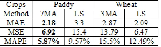
Table 6 shows the error measures of MA methods by applying the error measures MAE ,MSE & MAPE. After analysis of this table value we shows that 3 yearly moving average has minimum errors in production of paddy.7 yearly moving average has minimum errors for wheat production.

4.3 Least Square Methodand error measures based on this method: In this section at first we obtain the Least Square Method results by using formulas. Table(7) shows actual and estimated values of paddy production by least square method. The figure(3) shows the same results graphically for better understanding of the smoothness of the data. Similarly Table (8) and figure (4) shows the result of least square method by taking the same length of year for wheat production and also provide its smoothness based on least square method.

Table(7) Actual and estimated values of paddy production by least square method

Figure(3): The trend of least square method of paddy production

9 | P a g e

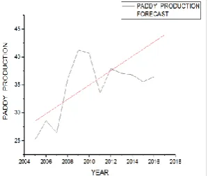
By comparing the tables 7 and 8 the performance of the methods by Moving Average and Least square method on the basis of MAE ,MSE and MAPE the following table is found which has less error and more accuracy than the other method.

Table(9):Error Measure of Least Square Method

After evaluating the error measures, next we are going to discuss our results in the following section .

10 | P a g e

In the previous section, two valid methodologies namely Moving average and Least square methods are used to predict future data. In section 3 detail of wheat and paddy production of Punjab Mandi board , Mohali Chandigarh for the period of 2005-06 to 2016-17 is provided for our study concern. In this paper we forecast the future data of both, paddy and wheat for the period of 2017-18. For this purpose we applied the methodology of minimum error method. In this study we ignore the large errors, which are the sometime primary concern. But sometimes large errors created disproportionate impacts for forecasting future data. So the selection of an error measure is dependent upon the situation. None of the error measures was superior on all criteria. In this paper the performance of the various methods are evaluated on the basis of MAE, MSE and MAPE .

Table 10: Diagnostic measures for the selection of the best forecasting method for wheat and paddy

production

The above table shows errors of paddy and wheat production on the basis of MAE,MSE and MAPE. In case of production of paddy the error value of moving average on the basis of MAE , MSE and MAPE are less as compare to least square method. On the other hand for the production of wheat, the error values of least square method are smaller than the moving average method on the basis of MAE, MSE and MAPE .

By comparing the performance of these method it has been found that according to data set we have selected the best method for forecast the future data. Therefore in this study we select the moving average method is appropriate for forecasting the future data of paddy production and on the other hand the least square method is appropriate for forecasting the wheat production and it is because of their least error measures in terms of MAE, MSE and MAPE are less.

VI. CONCLUSION

In this paper, an attempt is made to obtain forecast of paddy and wheat production , Punjab, India. Analysis is based on time series of past production. We explored the impact of using methodologies based on error measures. Forecasting of wheat and paddy production done by using statistical methods (Moving average Method, Least square method). Statistical method are chosen because of their rich historic data and ease of their use . Finally their performance evaluated by comparing the MAE, MSE and MAPE obtained from the different methods .The result shows that the moving average method is more accurate average method for the production of paddy whereas the production of wheat we find least square method is more accurate method on the basis of error estimation process .

The forecasting technique may be differed for different areas . It depends on variable factor. Hence this work may be extended to other agriculture areas.

11 | P a g e

The authors wish to thank the Guru Kashi University for providing research opportunities and support . We would also like to thank Punjab Mandi Board ,Mohali ,Chandigarh for providing us the valuable data for our use.

REFERENCES

[1.] Brockwell, P.J., and Davis, R.A.1996”Introduction to time series and forecasting “Springer

[2.] Jan G. De Gooijer , Rob J. Hyndm”25 years of time series forecasting” , International Journal of Forecasting 22 (2006) 443– 473

[3.] Michael Lawrence, Paul Goodwin, Marcus O'Connor, Dilek Önkal (2006) “Judgmental forecasting:“A review of progress over the last 25 years” International Journal of Forecasting, Volume 22,Issue 3, Pages

493-518.

[4.] S. Skakun1,2, B. Franch1,2, J.-C. Roger1,2, E. Vermote2,”Incorporating yearly derived winter wheat yield

forecasting model” I. Becker-Reshef1, C. Justice1, A. Santamaría-Artigas1

[5.] Cordery, I., and A.G. Graham. 1989. Forecasting wheat yields using water budgeting model. Aust. J. Agric. Res. 40:715–728

[6.] Rakesh Kumar & Dalgobind Mahto” Application of proper Forecasting technique in juice production :A

case study “Global Journal Of Researches In Engineering Industrial Engineering, vol-13 issue 4 version 1.0

year 2013

[7.] Satya Pal, Ramasubramanium V. and S.C. Mehta (2007)“Statistical models for milk production in India” Journal of Indian society of Agriculture and statistical 61 (2), 2007 80-83

[8.] Parth Parekh, Vaibhavi Ghariya” Analysis of moving average methods “International Journal of Engineering and Technical research” Vol-3, Issue-I,January 2015

[9.] M.A.K. Khalil & F.P. Moraes “Linear Least Squares Method for Time SeriesAnalysis with an Application to a Methane TimeSeries” Journal of the Air & Waste Management Association ,year2012

[10.] Rob J Hyndman”Moving averages” International Journal of Forecasting 22,November 8, 2009

[11.] R. B. MacDonald and F. G. Hall “Global Crop Forecasting “,Internationalt rade de, SCIENCE, VOL. 208, 1980

[12.] Lihong Xue and Dongping Li “Research on Piecewise Linear Fitting Method Based on Least Square Method in 3D Space Points”The Open Automation and Control Systems Journal, 2015, 7, 1575-1579

[13.] Steven J. Miller “The Method of Least Squares” Mathematics Department, Brown University [14.] Providence, RI 02912

[15.] Makridakis, S., 1993. Accuracy measures: theoretical and practical concerns,International Journal of Forecasting 9, 527–529.

[16.] Rob J. Hyndman , Anne B. Koehler “Another look at measures of forecast accuracy”, International Journal of Forecasting 22 (2006) 679–688

[17.] Armstrong, S., Collopy, F., 1992”Error measures for generalising about forecasting methods: empirical comparisons” International Journal of Forecasting 8, 69–80.

12 | P a g e

[20.] T. Chai1,2 and R. R. Draxler Root mean square error (RMSE) or mean absolute error (MAE)? – [21.] Arguments against avoiding RMSE in the literature

[22.] Yi-Shian Lee, Lee-Ing Tong (2011) “Forecasting time series using a methodology based onAutoregressive integrated moving average and genetic programming” Knowledge-Based Systems

[23.] 24 (2011) 66–72.