ISSN (e): 2250-3021, ISSN (p): 2278-8719
Vol. 08, Issue 5 (May. 2018), ||VI|| PP 24-32
A Novel Image Classification Method Using Texture Feature
Descriptors
Anto.A.Micheal
1, Anand. T
2,
1Department of Computer Science and Engineering, Secunderabad, India. Swami Vivekananda Institute of Technology,
2Department of Computer Science and Engineering, Swami Vivekananda Institute of Technology, Secunderabad, India.
Corresponding Author: Anto.A.Micheal
Abstract:
In computer vision, image classification has become an important task to automatically detect objects. Image classification is referred as labeling the images into one of the many predefined categories. Difficulties confronted in classifying the objects prompted the researchers to broaden new solutions to represent visual information. This paper proposes a classification model using the combination of GLCM, HOG, LBP and Gabor features. This proposed approach extracts texture features like GLCM, HOG, LBP and Gabor features from the image. Firstly, the images are classified with GLCM features, secondly they are classified with HOG, LBP and Gabor features, and finally they are classified with the combination of GLCM, HOG, LBP and Gabor features using Naïve Bayes, Adaboost and Random Forest algorithms. The proposed approach is experimented on Caltech101 image database and their performances are evaluated using accuracy, precision and recall parameters. The statistical result shows that the accuracy, precision and recall are 92%, 0.92 and 0.94 respectively. The comparative study shows that classifying the image datasets with the combination of GLCM with HOG, LBP and Gabor features gives the better classifying result than classifying separately.Keywords:
Image Classification, Caltect101 Dataset, GLCM, HOG, LBP, Gabor, Adaboost--- Date of Submission: 23-04-2018 Date of acceptance: 11-05-2018 ---
I.
INTRODUCTION
Nowadays images are broadly utilized because of its visual representation. Classification of the objects is an easy task for humanity, but its challenging task for the machine. The image data can take many forms, such as video sequences, views from multiple cameras, etc (Oliver et al., 2000). Methods of computer vision are computer human interaction, event detection, object identification, Object recognition, object classification and object tracking. The image classification includes image pre-processing, object detection, object segmentation, feature extraction and object classification. The Image Classification framework comprises of a database with predefined patterns that compare with an object to classify to appropriate category. Image Classification is an important task in various fields such as remote sensing, biometry, biomedical images, and robot navigation.
A traditional classification system consists of a camera fixed high on the intrigued zone, where images are captured and consequently processed. There are two types of classifications; they are supervised classification and unsupervised classification (Jianxin, 2012). In supervised classification, the image dataset is partitioned into training dataset and testing datasets. In training dataset the images are grouped into different classes and these training datasets are used to train the classifier model. The classifier model is tested using testing dataset. In unsupervised classification, the images are grouped with the help of their properties, these groups are known as clusters. This process is also known as clustering. In Image classification consists of different classification algorithms they are; Decision Tree, Artificial Neural Network (ANN), Support Vector Machine (SVM) etc.
In this paper, texture feature descriptors (GLCM, HOG, LBP and Gabor) are extracted for image classification. The motive was to extract complimentary information from the various texture descriptors from an image and classify them. The classification algorithms used are Naïve Bayes, Adaboost and Random Forest algorithms to classify images from databases. The classification algorithms are evaluated using accuracy, precision and recall parameters.
II.
LITERATURE SURVEY
Image Classification refers to the task of extracting information from an image. The primary objective of image classification is to detect, identify and classify the features occurring in an image in terms of the type of class these features represent on the field (Gabrya & Petrakieva, 2004). Image Classification can be broadly divided into supervised and unsupervised. Many algorithms are proposed for image classification. It is difficult to analyze the best classification algorithm as numerous factors affect the results. The researches show that Minimum distance classifier is highly recommended in all image classification applications due to its minimum computation time as it depends mainly on the training data, it is also said that it works best in applications where spectral classes are dispersed in feature space and have similar variance.
The Fuzzy C Means clustering algorithm has been widely used in image segmentation since it was proposed (Jia et al., 2009). In Comparison to Hard c-means algorithm FCM is able to preserve more information from the original image. However, it is noise-sensitive as it does not take into account the spatial information of a pixel (Jia et al., 2009). The supervised Fuzzy C means as proposed for security assessments provides high accuracy and less computational effort (Kalyani & Swarup, 2010). K-Nearest Neighbor provides fast, objective, transparent and produces good results over larger areas. The importance of KNN methods is its simplicity and lack of parametric assumptions (Mayanka, 2013). It is different from other classification methods as it does not take into account the mean of the class pixels.
The literature of Maximum likelihood method describes that it needs longer time of computation relies heavily on a normal distribution of the data in each input band and tends to over-classify signatures with relatively large values in the covariance matrix (Ahmadi & Hames, 2009). However, it requires the least computational time amongst other supervised methods as the pixels that should not be unclassified become classified, and it does not consider class variability (Gabrya & Petrakieva, 2004). The results of supervised classification depend on the quality of training data.
III.
PROPOSED METHODOLOGY
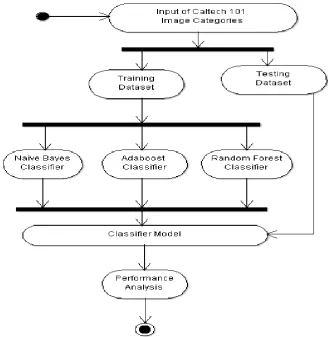
Figure 2: Business modeling for image classification
3.1 Feature Extraction: a) GLCM:
Gray Level Co-occurrence Matrix (GLCM) is used to calculate the special dependence of gray levels in an image (Vijayakumar et al., 2015). In GLCM the number of rows and columns are exactly equal to the number of gray levels in the image. Co-occurrence matrices are constructed in four spatial orientations (0, 45, 90 and 135). Another is constructed as the average of preceding matrices. Let the Co-occurrence matrix be Pi,j and the size of the matrix is NxN. Each element (I,j) represents the frequency by which pixel with gray level I is spatially related to pixel with gray level j. Construction of GLCM gram a gray scale image (Mattonen, 2014) is illustrated in Figure.2. The sample input image consists of 10 gray levels. GLCM represents the relation between reference pixel (i) and the neighbor pixel (j) in various orientations (Robert, 1979). Here the relation between pixels is calculated horizontally towards the right (0). Initially, the value of each element in GLCM (i,j) is Zero. The value of each element is updated as per the occurrence of pixels together. Texture features are calculated using GLCM are contrast, correlation, homogeneity, energy and there equations are shown from Equation (1) – (4) respectively.
Contrast =
1
0 ,
2 ,
(
)
Nj i
j i
i
j
P
- (1)Correlation =
1
0 ,
2 2 ,
N
j
i i j
j i
j i
j
i
P
- (2)
Energy =
1
0 ,
, 2 N
j i
j i
Homogeneity =
1 0 , 2 ,1
N j i j ij
i
P
- (4)b) HOG Features:
HOG features, which were firstly connected for human detection (Dalal & Triggs, 2005) are computed by counting the occurrences of gradient orientation in localized portions of an image. HOG features are based on the fact that the appearance and shape of the facial features can be depicted by the distribution of intensity gradients. The features so acquired are profoundly discriminative and represent an image characteristic faithfully (Nascimento & Sridhar, 2003; Mavadati et al., 2013). Motivated by the significant results from feeling acknowledgment, HOG features are adopted for image classification. The gradient oriented histogram is computed in Equation (5) – (10) as follows:
k ij d d ijm
k
h
- (5)2 2
ij ij ij
dx
dy
m
- (6)D
dx
dy
d
ij ij ij
arctan
- (7)j i ij ij
I
I
dx
1, - (8)j i ij ij
I
I
dy
1, - (9)
ij ij ij ijdx
dy
D
arctan
- (10)Where
I
ij is thei
,
j
pixel value of each sub-region,m
ij is the Gradient magnitude of the pixeli
,
j
is the gradient direction at pixel
i
,
j
,h
(k
)
is the kth dimensionh
(k
)
of the gradient histogram represents the total intensity of the pixel gradient whose direction lies in the kth direction bin dk, k = 0 to7. The direction bins are defined by the relative angle to the dominant gradient direction D of the image region. Finally, combing all the Gradient orientation Histogram of the interest point’s area together to form a feature vector of size 128-dimension.c) LBP Features:
LBP features are observed to be a capable technique for texture feature extraction and have been popularly accepted for image representation (Feng et al., 2007; Shan et al., 2009). The most important properties of LBP are computation simplicity and illumination invariance. Moore and Bowden (Moore & Bowden, 2011) has explored numerous variants of LBP for multi-view image representation to investigate the importance of multi-resolution and orientation analysis for feature representation. We have used extended LBP, which is rotation invariant. Rotation invariant LBP utilizes fewer bins as compared to consistent LBP and reduces the quantity of components used for binary pattern representation.
Feature extraction is implemented as follows: to start with, the image is divided into several non-overlapping blocks. Then, LBP histograms are calculated for each block. Finally, the block LBP histograms are concatenated into a single vector. Therefore, the images are represented by the LBP and the shape is recovered by the concatenation of different local histograms.
Formally, given a pixel at
x
c,
y
c
the resulting LBP can be expressed in decimal form as equation (11):
10
,
,
2
p p p c p c c R
P
x
y
s
i
i
LBP
- (11)where
i
c andi
p are respectively gray-level values of the central pixel and P surrounding pixels in thecircle neighborhood with a radius R, and function
s
x
is defined as in equation(12):d) Gabor Features:
Gabor filters have been utilized widely in image processing, texture analysis for their excellent properties: optimal joint spatial\spatial-frequency localization and the capacity to simulate the receptive fields of simple cells in the visual cortex (Rashedi & Nezamabadi-pour, 2012). Two-dimensional Gabor filter is a complex sinusoidal regulated Gaussian function with the response in the spatial domain (Equation (13)) and in spatial-frequency domain (Equation (14)).
1 2 2 2 2 2 12
.
exp
2
1
exp
2
1
)
,
,
,
;
,
(
x
y
R
R
X
i
R
h
Y x y x yx , - (13)
Where,
,
sin
cos
1
x
y
R
,
cos
sin
2
x
y
R
2 2 2 2 1 2 21
2
exp
)
,
,
,
;
,
(
x
y
C
F
F
H
x
y
x
y - (14)Where,
,
sin
cos
1
u
v
F
C = constant,,
cos
sin
2
u
v
F
3.2 Classification Algorithms: a) Naïve Bayes Classifier:
The Naïve Bayes classifier found its way into many applications nowadays due to its simple principle, but yet powerful accuracy [20], [21] (Vidhya & Aghila, 2010; McCallum & Nigam, 1998). Bayesian classifiers are based on a statistical principle. Here, the presence or absence of a word in a textual document determines the outcome of the prediction. In other words, each processed term is assigned a probability that it belongs to a certain category. This probability is calculated from the occurrences of the term in the training documents where the categories are already known. When all these probabilities are calculated, a new document can be classified according to the sum of the probabilities for each category of each term occurring within the document. However, this classifier does not take the number of occurrences into account, which is a potentially useful additional source of information. They are called “naive” because the algorithm assumes that all terms occur independent from each other. Given a set of r document vectors
D
d
1,...,
d
r
classified along a setc
ofq
classes,
C
c
1,...,
c
q
, Bayesian classifiers estimate the probabilities of each classc
k given a documentd
jas equation (15):
j k j k j kd
p
c
d
p
c
p
d
c
P
- (15)In this Equation. 15,
p
d
i is the probability that a randomly picked document has vectord
jas itsrepresentation, and
P
c
k the probability that a randomly picked document belongs to ck. Because the number of possible documentsd
j is very high, the estimation ofp
d
jc
k
is problematic. To simplify the estimationof
p
d
jc
k
, Naive Bayes assumes that the probability of a given word or term is independent of other terms that appear in the same document. While this may seem an over simplification, in fact Naive Bayes presents results that are very competitive with those obtained by more elaborate methods. Moreover, because only words and not combinations of words are used as predictors, this naive simplification allows the computation of the model of the data associated with this method to be far more efficient than other non naive Bayesian approaches.Using this simplification, it is possible to determine
p
d
jc
k
as the product of the probabilities of each termthat appears in the document. So,
p
d
jc
k
may be estimated as in Equation (16):
T
i ij k k
j
c
p
w
c
d
p
1 - (16)
b) Adaboost Classifier:
Adaboost (Adaptive boosting) is a machine learning algorithm. It can be used with many different classifiers to improve the accuracy. Adaboost is adaptive in the sense that subsequent weak learners are tweaked (Zhang, 2013). Adaboost focuses on more previously misclassified samples. Initially, all samples are equal weights. Weight may change at each boosting round. It can be less susceptible to the over fitting problem than other learning algorithms. The individual learners can be weak, but as long as the performance of each one is slightly better and the final model can be proven to converge to a strong learner. Steps of Adaboost classifiers are Bootstrapping, Bagging, Boosting, and Adaboost. A boost classifier is a classifier in the form of Equation (17)-(18).
Tt t t
x
f
x
F
1
- (17)
Where
f
t is a weak learner that takesX
as input and the real value.
l
l t i t
t
E
F
X
h
X
E
1
- (18)Here
f
t1
x
is a boost classifier that built up a previous stage of training.c) Random Forest Classifier:
Random Forest developed by Leo Breiman (2001) is a group of un-pruned classification or regression trees made for the random selection of samples of the training data. Random features are selected in the induction process. A prediction is made by aggregating (majority vote for classification or averaging for regression) the predictions of the ensemble. By Sampling N randomly, If the number of cases in the training set is N but with replacement, from the original data. This sample will be used as the training set for growing the tree. For M number of input variables, the variable m is selected such that m is specified at each node, m variables are selected at random out of the M and the best split on this m is used for splitting the node. During the forest growing, the value of m is held constant. Each tree is grown to the largest possible extent. No pruning is used. Random Forest generally exhibits a significant performance improvement as compared to single tree classifier such as C4.5. The generalization error rate that it yields compared favorably to Adaboost, however, it is more robust to noise.
3.3 Performance Measures:
1) Accuracy: In the fields of science, engineering, industry, and statistics, the accuracy of a measurement system is the degree of closeness of measurements of a quantity to that quantity's actual (true) value and it calculated using equation (19).
TP
TN
TotalNumbe
r
Acc
- (19)2) Precision: In the field of information retrieval, precision is the fraction of retrieved documents that are relevant to the find. Precision takes all retrieved documents into account, but it can also be evaluated at a given cutoff rank, considering only the topmost results returned by the system. This measure is called precision calculated using equation (20).
TP
FP
TP
ecision
Pr
- (20)3) Recall: Recall in information retrieval is the fraction of the documents that are relevant to the query that are successfully retrieved. For example, for text search on a set of documents recall is the number of correct results divided by the number of results that should have been returned is calculated using equation (21).
)
(
Re
call
TP
TP
FN
- (21)IV.
DATASET
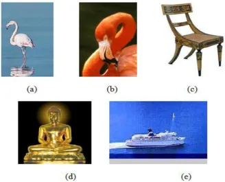
categories five categories are chosen for experimentation and they are shown in figure 3. Figure 3 consists of images taken from different categories such as flamingo, flamingo_head, chair, Buddha and ferry.
Figure 3: Image Datasets from 101Caltech database. a) Flamingo dataset, b) Flamingo_head dataset, c) Chair dataset, d) Buddha dataset, e) Ferry Dataset
V.
EXPERIMENTAL RESULTS AND DISCUSSIONS
The main aim of image classification is to calculate the accuracy of classified images based on the categories stated. The tests were performed on five categories that consist of seven features for each single image. A series of experiments was conducted using all features, each with a different number of training and testing images. Table 1 the results shows that the classification accuracy with the combination of GLCM, HOG, LBP and Gabor are using four different classifiers provides the highest accuracy with 92.00%.
Table 1: Comparison of Classification algorithms using different Texture Parameters Texture Features Classifier Accuracy Precision Recall
GLCM
Naïve Bayes 65 0.72 0.62
Adaboost 72 0.78 0.71
Random Forest 76 0.82 0.74
HOG, LBP, Gabor
Naïve Bayes 72 0.75 0.69
Adaboost 75 0.83 0.72
Random Forest 80 0.92 0.86
GLCM + HOG, LBP, Gabor
Naïve Bayes 84 0.86 0.82
Adaboost 92 0.94 0.91
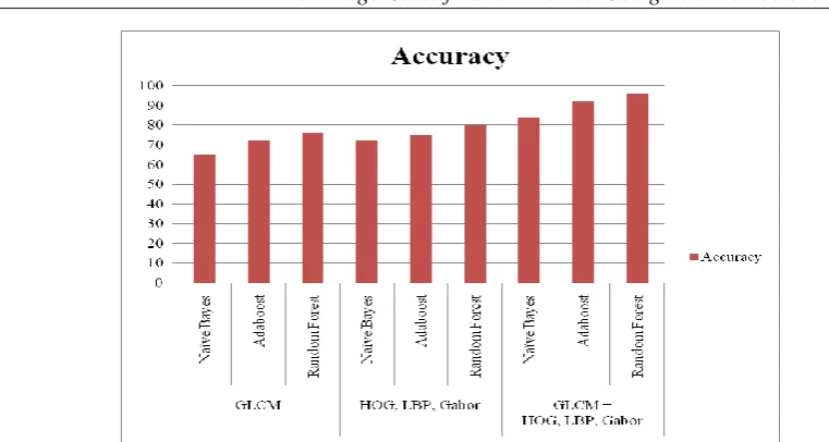
Figure 4: Analysis of different classification algorithms accuracy using texture features GLCM, (HOG,LBP,Gabor) and (GLCM+LBP,HOG,Gabor)
Figure 5: Analysis of precision and recall for different classification algorithms using texture features GLCM, (HOG,LBP,Gabor) and (GLCM+LBP,HOG,Gabor)
Table 1 shows that comparison classifying the dataset with texture features such as GLCM, HOG, LBP and Gabor and the combination of both GLCM and HOG, LBP and Gabor is respectively using Naïve Bayes, Adaboost and Random forest classifier. The classification algorithms are compared based on accuracy, precision and recall parameters. The dataset classified using Naïve Bayes, Adaboost and Random forest classifier with GLCM texture feature obtained accuracy as 65%, 72% and 76%, respectively, precision as 0.72, 0.78 and 0.82 and recall as 0.62, 0.71 and 0.74. The dataset classified using HOG, LBP and Gabor results in accuracy as 72%, 75% and 80%, respectively, precision as 0.75, 0.83, 0.92 and recall as 0.69, 0.72 and 0.86. The dataset classified using a combination of GLCM, HOG, LBP and Gabor with Naïve Bayes, Adaboost and Random Forest gives an accuracy of 84%, 92% and 96%. The precision is calculated as 0.86, 0.94 and 0.97 and recall as 0.89, 0.96 and 0.98 respectively. The graphical representation of comparison of accuracy and precision and recall is shown in Figure (4)-(5) respectively. The statistical result shows that the proposed method for classification has more accuracy, precision and recall than the existing methods. This implies that the texture feature with the combination of GLCM and HOG, LBP, Gabor classifies the dataset accurately than the GLCM and HOG, LBP, Gabor separately.
VI.
CONCLUSION AND FUTURE ENHANCEMENTS
existing methods. The classification performance of the proposed GLCM, HOG, LBP and Gabor feature in terms of accuracy, precision and recall are 90%, 0.92 and 0.94 respectively. In future, the classification system with different combination of texture features in the domain like crime prevention, medical diagnosis, intellectual property and textile industry can be experimented and performed.
REFERENCES
[1] Ahmadi, F.S., & Hames, H.S. (2009). “Comparison of Four Classification Methods to Extract Land Use and Land Cover from Raw Satellite Images for Some Remote Arid Areas”, JKAU; Earth Science, 20(1), 167-191.
[2] Breiman, L., (2001). “Random Forests”, Machine Learning, 45(1),5-32.
[3] Dalal, N., & Triggs, B. (2005). “Histograms of oriented gradients for human detection”, Proceedings of the IEEE Computer Society Conference on Computer Vision and Pattern Recognition, CVPR 2005, pp. 886–893, San Diego, CA, USA.
[4] Fei-Fei, L., Fergus, R., & Perona, P. (2007). “Learning Generative Visual Models from Few Training Examples: An Incremental Bayesian Approach Tested on 101 Object Categories,” Computer Vision and Image Understanding, 106, 59-70.
[5] Feng, X., Pietikainen, M., & Hadid, A. (2007). “Facial expression recognition with local binary patterns and linear programming”, Pattern Recognition and Image Analysis, 17(4), 592–598.
[6] Gabrya, B., & Petrakieva, L (2004). “Combining labeled and Unlabelled data in the design of pattern classification systems”, International Journal of Approximate Reasoning, 35(3), 251-273.
[7] Jianxin Wu. (2012). “Efficient HIK SVM Learning for Image Classification”, IEEE Transactions on Image Processing, 21(10), 4442 – 4453.
[8] Jia, K., Cheng-Long, G., & Wen-Juan, Z. (2009). “Fingerprint image segmentation using modified fuzzy c-means algorithm”, Journal of Biomedical Science and Engineering, 2, 656-660.
[9] Kalyani, S., & Swarup, K.S. (2010). “Supervised fuzzy c-means clustering technique for security assessment and classification in power systems”, International Journal of Engineering, Science and Technology, 2(3), 175-185
[10] Mattonen, S., Huang, K., Ward, A., Senan S., & Palma, D. (2014). “New techniques for assessing response after hypo fractionated radiotherapy for lung cancer”, Journal of Thoracic Disease, 6(4), 375-386.
[11] Mavadati, S., Mahoor, M., Bartlett, K., Trinh, P., & Cohn, J. (2013). “DISFA: A spontaneous facial action, intensity database”, IEEE Transactions on Affective Computing, 4(2), 151–160.
[12] Mayanka, B.K. (2013). “Classification of Remote Sensing data using KNN method”, Journal Of Information, Knowledge And Research In Electronics And Communication Engineering, 2(2), 817-821. [13] McCallum, A, & Nigam, K. (1998). “A Comparison of Event Models For Naïve Bayes Text
Classification”, In the Proceedings of the Workshop on Learning for Text Categorization, 41-48.
[14] Moore, S., & Bowden, R. (2011). “Local binary patterns for multi-view facial expression recognition”, Computer Vision and Image Understanding, 115(4), 541–558.
[15] Nascimento, X. L. M.A., & Sridhar, V. (2003). “Effective and efficient region-based image retrieval”, Journal of Visual Languages and Computing, 14(2), 151-179.
[16] Oliver, Nuria, M., Barbara, & Alex P. (2000). "A Bayesian computer vision system for modeling human interactions”, IEEE Transactions on Pattern Analysis and Machine Intelligence, 22(8), 831-843.
[17] Park, B., & Lee, J.W. (2004). “Content-based image classification using a neural network,” Pattern Recognition Letters, 25(3), 287-300.
[18] Rashedi, S. S. E., & Nezamabadi-pour, H., (2012). “A simultaneous feature adaptation and feature selection method for content-based image retrieval systems,” Knowledge-Based Systems, 39, 85-94, 2012. [19] Robert M., (1979). “Statistical and structural approaches to texture”, Proc. IEEE, 67(5), 786-804, 1979. [20] Shan, C., Gong, S., & McOwan, P.W. (2009). “Facial expression recognition based on local binary
patterns: a comprehensive study”, Image and Vision Computing, 27(6), 803–816.
[21] Vidhya, K. A., & Aghila, G. (2010). “A Survey of Naïve Bayes Machine Learning approach in Text Document Classification”, International Journal of Computer Science and Information Security, 7(2), 206-211.
[22] Vijayakumar, V., Neelanarayanan, V., Veeramuthu, A., Meenakshi, S., & Priyadarsini, V. (2015). “Brain Image Classification Using Learning Machine Approach and Brain Structure Analysis”, Procedia Computer Science, 50, 388-394.
[23] Wang, H. Y. X. Y., & Yua, Y.J. (2011). “An effective image retrieval scheme using color, texture and shape features”, Computer Standards & Interfaces, 33(1), 59-68.