DOI 10.1007/s13173-012-0072-8 W T I
Partially labeled data stream classification
with the semi-supervised
K
-associated graph
João Roberto Bertini Jr.·Alneu de Andrade Lopes· Liang Zhao
Received: 15 June 2011 / Accepted: 22 March 2012 / Published online: 17 April 2012 © The Brazilian Computer Society 2012
Abstract Regular data classification techniques are based mainly on two strong assumptions: (1) the existence of a reasonably large labeled set of data to be used in training; and (2) future input data instances conform to the distribu-tion of the training set, i.e. data distribudistribu-tion is stadistribu-tionary along time. However, in the case of data stream classifica-tion, both of the aforementioned assumptions are difficult to satisfy. In this paper, we present a graph-based semi-supervised approach that extends the static classifier based on theK-associated Optimal Graphto perform online semi-supervised classification tasks. In order to learn from la-beled and unlala-beled patterns, here we adapt the optimal graph construction to simultaneously spread the labels in the training set. The sparse, disconnected nature of the proposed graph structure gives flexibility to cope with non-stationary classification. Experimental comparison between the pro-posed method and three state-of-the-art ensemble classifica-tion methods is provided and promising results have been obtained.
This is a revised and extended version of a previous paper that appeared at WTI 2010 (III International Workshop on Web and Text Intelligence) and has been recommended to JBCS.
J.R. Bertini Jr. (
)·A.A. Lopes·L. ZhaoInstituto de Ciências Matemáticas e de Computação, USP, Avenida Trabalhador São-Carlense, 400, 13566-590 São Carlos, Brazil
e-mail:[email protected]
A.A. Lopes
e-mail:[email protected]
L. Zhao
e-mail:[email protected]
Keywords Semi-supervised online classification· Incremental learning·Graph-based learning· Concept drift
1 Introduction
Recently, graph-based (also referred to network-based) al-gorithms applied to data mining tasks have attracted great attention in both theoretical research and practical applica-tions [5]. This growing interest is mostly justified due to the advantages provided by graph representation, such as reveal-ing topological structure of input data and the ability of iden-tifying arbitrary shapes of data clusters [27]. In such graph-based algorithms, each vertex of the graph represents a data pattern (data instance) and the edges stand for some relation of similarity between vertices. In order to reveal significant relations within a data set, the following rule is usually con-sidered for establishing connections between data patterns: the higher the similarity among data, the higher the proba-bility of connection [39]. Stated in this way, nearby patterns tend to be heavily linked together while distant patterns may form a sparse structure. This property has been extensively explored using graph-based solutions, especially consider-ing unsupervised tasks like clusterconsider-ing [32] and dimension-ality reduction [1]. Only recently graph-based classification has been addressed, usually by the wrap of semi-supervised learning [38].
For example, consider obtaining enough labeled data to train a classifier for a spam detection task (i.e. classifying spam and valid email). Such application design (1) incurs cost in paying an expert or a group of users to label what they call spam from what they consider real email; (2) may result in inconsistencies if we accept all human categorization. For instance, an email message may be considered as a spam by some people, but it may be considered as a valid email by others; (3) not to mention the time required to manually label enough data to train a regular supervised learning method.
A spam detection application is really a stream classifi-cation problem, in the sense that the classifier needs to clas-sify new patterns at the time they arrive [35]. In this kind of applications, the underlying data distribution changes over time, and such changes often make the model built on old data inconsistent to the newly arrived data. This problem, known as concept drift [34], requires frequent updating of the model. Summarizing, we have a classification problem which consists of a data stream where few instances are la-beled and data distribution may change over time. This sce-nario poses a challenging task for machine learning because it presents too few labeled data along the stream to apply a supervised incremental algorithm and the presence of con-cept drift disables the use of static classifiers. In fact, only recently such applications have been properly addressed due to the concept of learning through both labeled and unla-beled data and the development of semi-supervised learning strategies.
In the development of semi-supervised learning algo-rithms, many efforts have been made on the use of a clus-tering algorithm to group the patterns and further spread the labels. When considering this approach, the K-means algorithm is a natural choice. Li et al. [20] proposed a tree-based algorithm which uses the K-means to spread labels at the leaves of a tree. Masud et al. [22] proposed an en-semble of micro-clusters, obtained by using the K-means algorithm, then instances are classified according to the K-nearest neighbor rule. Ditzler and Polikar [11] proposed an ensemble of classifiers, named WEA, which are trained with labeled patterns only. Then, unlabeled data and theK-means algorithm are used to generate a mixture of Gaussian mod-els for further adjusting the weights of each classifier. Zhang et al. [37] use the semi-supervised SVM [8] allied to a ver-sion of theK-means, referred to as relationalK-means, to construct new features to the labeled examples by using in-formation extracted from unlabeled instances. Some inves-tigations have been made to tackle specific problems, e.g. Erman et al. [12] proposed a method to perform traffic clas-sification in computer networks with partially labeled data. Their method uses a clustering algorithm, such asK-means, to obtain the clusters and then, the labels are spread using the maximum likelihood estimation. The clusters that re-main unlabeled are likely to be an undefined group. Also
regarding computer network, Yu et al. [36] have considered the problem of intrusion detection. They employ a strategy similar to the K-means by grouping the labeled data and then, the labels are spread to the whole data set according to the distances from the clusters to unlabeled patterns. Finally, a SVM is trained to detect intrusion.
To the best of our knowledge, graph-based approach has not been considered to tackle streaming classification prob-lems where data are partially labeled; although it is success-fully applied to semi-supervised learning, especially to the transduction problem [2,6,10,25]. In view of the recent developed graph-based nonparametric classification method and its good performance on stationary data sets [4,21]; we had proposed a non-stationary version with initial results re-ported in Ref. [3]. In this paper, we propose an extended version to be applied in the context of non-stationary stream of partially labeled data. The aforementioned graph-based method is based on representing the training set as a special graph, referred to asK-associated graph. TheK-associated graph is able to represent similarity relations among data in-stances and the purity of a component (connected subgraph) is able to represent the data topology. Purity characterizes the degree in which instances of different classes are mixed in a same region of the data space. In this work we propose a new constructing procedure for the K-associated graph that takes into account partially labeled sets. Also, this work shows how the graph is updated along the time to allow data stream processing.
The remainder of the paper is organized as follows: In Sect.2, we briefly describe the problem of concept drift and also a toy example to illustrate a scenario where incremen-tal learning is applicable. Section3 presents the proposed method for non-stationary partially labeled stream classifi-cation. This section is further divided into four subsections, where Sect. 3.1 first introduces the K-associated graphs and the K-associated optimal graph. The new method for constructing the aforementioned graphs from partially la-beled data sets is described in Sect.3.2. Moreover, Sect.3.3 briefly treats the static KAOG classifier [4] and Sect.3.4 de-tails how the graph is updated over time. Section4presents the experimental results concerning the performance com-parison between the proposed algorithm and three well-know fully supervised streaming ensemble classifiers on non-stationary partially labeled benchmarks. Section5 con-cludes the paper and discusses some future works.
2 Background
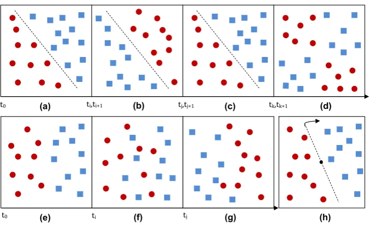
Fig. 1 Frequent concept drift characterizations, (a)–(d), abrupt drifts with recurrence; (e)–(g) gradual drift and (h) example subjugated to the velocity it is modified
given period of time. In the literature, however, the term con-cept drift has been used in reference to different phenomena relating to drop down the classifier accuracy performance [31]. According to Kelly et al. [17], concept drift occurs due to alterations on the following probabilities of data produc-tion:
– A prioriof classesP (ω1), . . . , P (ωM), i.e. alteration on
the relative size of a given class or the appearance of new classes.
– ConditionalP (x|ωi), i.e., changing on class definition.
For example, changes in the shape of a class.
– Conditionala posterioriP (ωi |x), i.e., modification on
some of the attributes;
In general terms, concept drift can be characterized ac-cording to the variation of the concepts mainly regarding two features,velocityandrecurrencealong the time. Basi-cally, in the former, a concept drift can be divided into grad-ual driftandabrupt drift; while in the latter, a concept drift isrecurrentif past concept turns to be current concept. Both kinds of concept drift are sketched in Fig.1.
In Fig. 1, the (blue) rectangles represent the instances that belong to class ω1 and the (red) circles represent the
instances belonging to classω2. Consider Figs.1(a)–(d) as a
sequence of data distributions of an application presented in time, initiating at t0. The concept drifts that occur
be-tween distributions of Figs. 1(a) and 1(b), as well as be-tween Figs. 1(b) and 1(c), are abrupt. Also notice that the distribution shown by Fig.1(c) is similar to that in Fig.1(a), which mean that the distribution at timet0in Fig.1(a) occurs
again at time tj+1, after experiencing a completely
differ-ent distribution (Fig.1(b)). This phenomenon characterizes a recurrent concept. As the time line shows, from Figs.1(a) and1(d), each distribution can, eventually, remain static for
a given period of time, e.g., the initial distribution remains static fromt0 toti. Nonetheless, on the next iterationti+1,
the distribution can be totally altered, i.e. an abrupt drift oc-curs. The drift between distributions in Figs.1(c) and1(d) is also considered abrupt, in spite of being less severe than the previous one. Consider now a situation where two groups of data from different classes cross each other along time, depicted in order in Figs.1(e)–(g), from an initial distribu-tion (Fig.1(e)) to a final one (Fig.1(g)) with Fig.1(f) corre-sponding to an intermediate distribution. In such a scenario, the distribution varies smoothly throughout the time, which characterizes a gradual drift. At last, let Fig.1(h) represent a distribution determined by a rotating hyperplane along the time. If the hyperplane is rotated byπ/4 regularly at a given period of time, the drift is characterized as gradual and re-current at every eight alterations of the hyperplane. How-ever, if the angular velocity rate is increased, say toπ, the drift now can be considered abrupt. This demonstrates that it is surprisingly difficult to accurately characterize concept drifts considering only velocity and recurrence. In view of this problem, many researchers have proposed different drift categories; for a recent work, refer to Ref. [23].
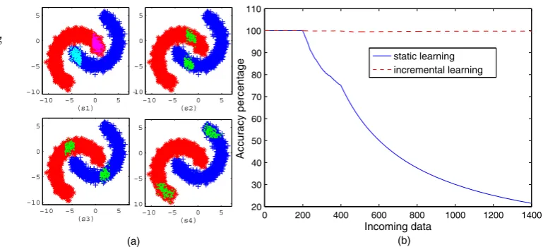
Fig. 2 (a) Artificial data set (Banana set) divided into sequential groups for simulating a non-stationary domain. The highlighted examples represent those chosen examples in a run. (b) Cumulated accuracy for static and incremental learning using the KAOG classifier
drift; (iii) selecting what data should be used to train the new classifier is also a hard task. Fortunately, incremental learn-ing algorithms can be applied to provide practical solutions to tackle classification problems on non-stationary domains. Such an approach enables a classifier to acquire knowledge during application phase, updating the model with new data, and without explicitly retraining itself [14,30].
For clarifying the advantages of an incremental classi-fier over a static one in non-stationary domains, consider the following experiment with the artificial data set known as banana set (see Fig.2(a)). The experiment consists of com-paring both approaches, static and incremental, of the clas-sifier based on theK-associated graph. For doing so, in both cases, the classifier is trained with a limited subset (set “s1” in Fig.2(a)). The rest of the set is divided into seven groups and used as test sets that are sequentially presented to the classifier. In Fig. 2(a) “s1” is the original training set and the others correspond to the first, second, and seventh test sets, respectively. The results are averaged over 10 runs, at each run, an optimal graph is built considering 400 exam-ples (200 of each class) randomly chosen from the train-ing data group. After traintrain-ing, the test examples are chosen obeying the group sequence, one-by-one, 200 examples are randomly chosen from each group (100 for each class), then, the next group takes place and so on.
Figure2(b) shows the results of the comparison between theK-associated static and incremental classifiers. The sig-nificant difference between them is due to the fact that the static classifier no longer learns with new instances, how-ever the incremental classifier is able to learn during classi-fication phase. The presented incremental learning process is analogous to the linearization technique widely used to study local properties of non-linear systems. Specifically, linearization of a neighborhood of a certain point corre-sponds to subset selection in incremental learning. Non-linearity of the system corresponds to twisted shape of classes and changing of data distribution over time. In a non-linear systems, linearization usually can obtain good
approximation if the neighborhood under analysis is small. For the same reason, we expect that good classification re-sults can be obtained by updating the network with small data subset each time.
3 The semi-supervisedK-associated optimal graph
The semi-supervised K-associated graph, proposed here, consists of a modification of the K-associated graph [4] to deal with both labeled and unlabeled data during the graph construction procedure. Therefore, in order to intro-duce the semi-supervised version, a brief revision of the K-associated graph is presented in Sect.3.1. It is followed by the semi-supervised K-associated graph construction pre-sented in detail in Sect. 3.2. Both supervised and semi-supervisedK-associated optimal graphs can be seen as the training process for the KAOG classifier which uses the components of the graph and their purities to classify new data instances, as will be exposed in Sect.3.3.
3.1 TheK-associated graph and theK-associated optimal graph
A K-associated graph is constructed from a vector-based data setX= {x1, . . . ,xN}by representing each data instance xi =(xi1, xi2, . . . , xip, ci)as a vertexvi with its associated
class label ci, where ci ∈Ω = {ω1, ω2, . . . , ωM} and M
is the number of classes in the problem. The graph con-struction resembles to aKNN graph, due to the use of a predefined number of neighbors,K, that each vertex must connect. Although theK-associated graph does differ from the KNN approach by the fact that amongst the possible K neighbors of a vertex vi, it can only be connected to
neighbors of the same class asvi. Hence, we consider the
represents the K nearest neighbors of the instance xi
ac-cording to a given measure and will be noted by Λvi,K. The latter comprises only the vertices with the same class as vi among its K nearest neighbors, and is defined as
Δvi,K= {vj|vj∈Λvi,KANDci=cj}.
In a formal way, theK-associated graph is defined as a directed graph G=(V , E) which consists of a set of la-beled verticesV and a set of edgesEbetween them, where an edge eij =(vi, vj)connects vertex vi with vertexvj if
and only ifvj∈Δvi,K. As a consequence, only vertices of the same class can be connected. The resultingK-associated graph can be viewed as a set of disjoint subgraphs or com-ponentsC= {C1, . . . , Cα, . . . , CR}. Each componentCα is
composed by vertices of a single class, thus each component represents a single class, which we refer to the label of com-ponentCα asCˆα. The number of componentsRvaries
ac-cording to the magnitude ofK, but always lies in the range N ≥R≥M, with N being the number of vertices in the training set andM the number of classes. Higher values of K induce fewer and larger components in the constructed graph, while lower values lead to small sized ones. This wire mechanism leads to a graph with some important features: (i) By varying K, different graphs can be generated, and as the value ofKincreases, the number of components de-creases monotonically to the number of classes. (ii) The total number of edges among the vertices of a componentCα is
proportional toKand can be at most equal toKNα, where
Nα is the number of vertices in componentCα. (iii) This
maximum value is only achieved if all vertices in the neigh-borhood of any vertex of the component have the same class. Likewise, nearby vertices of other classes decrease the num-ber of connections of the given component. Thus, one can define a measure of “purity” for components, as explained ahead.
Let the degreedi of a vertexvi be defined as the sum of
the connections it receives (in-degree) and the connections it performs (out-degree) to other vertices, sodi=diin+diout.
Also, consider the average degree taken for componentCα
be defined byDα=1/Nα
vi∈Cαdi. According to the way that theK-associated graph is constructed, a vertex can per-form at most K connections, thus, the maximal total out-degree of componentCα isKNα; symmetrically, the total
in-degree is also KNα, resulting in average degree being
equal to 2K. Hence, a key idea is to use the ratio defined in Eq. (1) as a measure of “purity” for componentCα, because
it quantifies how intertwined a component is with vertices of other classes,
Φα=
Dα
2K (1)
In this way, Φα =1, if and only if, for everyvi in the
componentCα, all theKneighbors have the same class label
ofvi. On the other hand, if there exists noise or two or more
classes are mixed together, vertices in this region are unable
to make theirKconnections due to the existence of vertices of other classes in the neighborhood of some vertices. In the latter case, the more mixing the components are, the lower their average degreesDα and consequently their respective
puritiesΦα are.
Clearly, the structure of a K-associated graph depends on the value ofK and on the nature of the input data set. Also, K-associated graphs formed with different K will present different components with different purity values. Bearing this in mind, a suggestive idea is to obtain a graph with the best organization of components without using a unique value of K, i.e., each component has its own opti-mal value ofK, denoted asKα for componentCα.
There-fore, the rationale for obtaining the optimal graph is to con-structK=1, . . . , Kmaxassociated graphs while keeping the
best components found at eachK throughout this process. Let β also be an index of component, therefore, a com-ponentCβ(K+z) from the (K+z)-associated graph will re-place all components from theK-associated graph that sat-isfy Eq. (2), for some integerz≥1 and(z+K)≤Kmax,
Φβ(K+z)≥Φα(K) for allCα(K)⊆C(Kβ +z) (2) The optimal graph improves the representation of the training set and provides the best configuration of compo-nents according to their purities. It corresponds to the best graph organization regarding the purity measure.
3.2 The semi-supervisedK-associated optimal graph
Consider now obtaining the optimal graph from a partially labeled setX. It is easy to see that it is not possible to ob-tain the aforementioned graph through the previous descrip-tion due to the presence of unlabeled patterns. Therefore, we propose here the semi-supervised construction of the K-associated optimal graph.
The problem addressed here regards the absence of enough labeled data in a given data set to employ a regular supervised method. Therefore, it is necessary to consider a semi-supervised method in order to induce a classifier from both labeled and unlabeled patterns. Hence, consider the data setX= {(x1, c1), . . . , (xl, cl),xl+1, . . . ,xN}withl
la-beled patterns (xi, ci)andN −l unlabeled patterns x (or
(xj,∅)). As its supervised counterpart, the semi-supervised
K-associated optimal graph construction involves creat-ing a sequence of semi-supervised K-associated graphs. The main difference between the supervised and semi-supervisedK-associated graphs can be stated in relation to the set of neighbors, to which each vertex connects. Instead of considering only the label-dependent set (Δvy,K), here, each vertex vi connects to all vertices in the set Γvi,K=
{vj |vj ∈Λvi,K AND (cj =ci ORci = ∅ OR cj = ∅)}. This set encompasses theK nearest neighbors ofvi whose
among itsKnearest neighbors,vi connects to those vertices
which belong to the same class ofvi or to those with no
la-bel. Ifvi itself does not have a class label, it connects to all
theKnearest neighbors without considering their classes. As a consequence of connecting unlabeled vertices to la-beled vertices regardless to their classes, components with more than one class may be formed. However, having com-ponents with more than one class precludes the classifier to make decisions. In other words, each component must be formed by vertices belonging to a single class and dif-ferent from null. Thus, to overcome this problem, we pro-pose splitting those components with vertices associated to two or more classes. For splitting a component, the ratio-nale is to cut a few edges in order to end up with separated well-connected clusters of vertices. In other words, this is a min-cut problem, which can be resolved, for example, by the Ford–Fulkerson algorithm [9] for the two-class case. How-ever, as we consider multi-class classification, there exists the problem that a component might be composed by ver-tices from more than two classes. For this reason, we pro-pose cutting the component based on the purity of vertex, de-fined asdi/2K, wheredi stands for the degree ofvi. Again,
considerWi,j the distance, used to construct the graph,
be-tween patternsxi andxj. Thus the proposed separation
ap-proach consists of successive removing the edge with mini-mum value of cut from the component, as defined in Eq. (3). Otherwise stated, the next edge to be removed(va, vb)∈Cα
must satisfy cuta,b=min(cuti,j)∀(vi, vj)∈Cα.
cuti,j =min
di
2K, dj
2K
1 Wi,j
(3) The cutting process in the component Cα finishes until
it is separated into single class components. The rationale behind the criterion is that by cutting the edges that con-nects low purity vertices and whose respective patterns are distant from each other, it is more likely to obtain separated well-connected components. In fact, low purity vertices are usually found in boundary regions between components of different classes in supervised tasks. However, in the semi-supervised scenario, purity itself can be a misleading mea-sure due to high connection probability of the unlabeled ver-tices. Therefore the distance weight in Eq. (3) favors cutting the edges with highest distance in the component.
Algorithm 1details the construction of the semi-super-vised K-associated optimal graph. The function findComponents()determines the graph components by im-plementing a breadth-first search [9]. Then, the components having vertices belonging to more than one class are sep-arated by the function splitNonSingleClassComponents(). This function implements the cutting procedure described earlier and returns two or more single class components, which can include components without a class label. The next step consists of spreading the labels within every com-ponent by calling the function spreadLabel(). After this
Algorithm 1Semi-supervisedK-associated Optimal Graph construction from partially labeled set—KAOGSS
Input: X= {(x1, c1), . . . , (xl, cl),xl+1, . . . ,xN}
Symbols: G(K)s —K-associated Graph built from labeled and unla-beled patterns
G(sopt)—K-associated Optimal Graph built from labeled and unla-beled patterns
Γvi,K—set ofKnearest neighbors ofvi within the same label or
no label
R—number of components in the current K-associated graph
G(K)s
M—the number of classes inX
1: K⇐1 2: repeat
3: C⇐ ∅
4: G(K)s ⇐ ∅ 5: for allvi∈Vdo
6: Γvi,K⇐ {vj|vj∈Λvi,K and(cj=ciorci= ∅or
cj= ∅)}
7: E⇐E∪ {eij|vj∈Γvi,K}
8: end for
9: C⇐findComponents(V , E)
10: C⇐splitNonSingleClassComponents(C)
11: for allCα∈Cdo
12: Cα⇐spreadLabel(Cα) 13: Φα⇐purity(Cα)
14: G(K)s ⇐G(K)s ∪ {(Cα(V, E);Φα)} 15: end for
16: ifK=1then 17: G(sopt)⇐G(K)s
18: else
19: for allCβ(K)⊂G(K)s do 20: for allC(αopt)⊆C(K)β do
21: if(Φβ(K)≥Φα(opt)orCˆα(opt)= ∅)then 22: G(sopt)⇐G(sopt)−
Cα(opt)⊆Cβ(K)
Cα(opt)
23: G(sopt)⇐G(sopt)∪
Cβ(K)
24: end if
25: end for
26: end for 27: end if 28: K⇐K+1 29: untilR=M
30: Output: TheK-associated optimal graph within all vertices with labelsG(opt)= {C1(opt), . . . , C(αopt), . . . , CR(opt)}where component
Cα(opt)=(G(V, E);Φα, Kα)
stage, all vertices in any given component are labeled with a single class label or are unlabeled. To finish the K-associated graph construction, the purity measure is calcu-lated through the functionpurity() for all components. At the end of this process, ifK=1, then the graph generated so far is the optimal graph and it is assigned toG(sopt).
Oth-erwise, each component of the currentK-associated graph, G(K)s , is compared to the components in the graph,G(sopt),
compo-nents. The process goes on by increasingK and generating a newK-associated graph until the number of components in this new graph matches the number of classes in the prob-lem(R=M).
In summary, the main modifications in the original K-associated optimal graph construction algorithm [4] include connecting each vertex to all its neighbors with the same class or without a class label (line 6) and merging every component with empty class (in the Algorithm1,Cˆα stands
for the class of a component) to another component, inde-pendent of purity. Notice that the present algorithm not only can construct the K-associated optimal graph, but also, by doing so, can spread the labels throughout the whole train-ing set. Therefore, the KAOGSS algorithm is a transductive method.
3.3 The KAOG classifier
This section presents the nonparametric classifier that uses the K-associated optimal graph structure to infer the class of new patterns, for more details, please refer to Ref. [4]. In order to present how a new pattern is classified, consider again a training patternxirepresented byxi=(xi1, xi2, . . . ,
xip, ci), whichxi represents theith training pattern withci
its associated class label, in a M-class problem ci ∈Ω =
{ω1, ω2, . . . , ωM}. In the same way, a new pattern is
de-fined asy=(y1, y2, . . . , yp), excepted that now its class
la-bel must be estimated. Consider also the set of components of the optimal graphC= {C1, . . . , Cα, . . . , CR}, whereRis
the number of components and R ≥M. In order to clas-sify the new pattern y, we must firstly transform it to a vertex, noted by vy, then connect it into the graph as
ex-plained ahead. ConsiderKLthe largest value ofKin the
K-associated optimal graph, or equivalently theKvalue from the last obtained component. For every new pattern y, we do:
1. Calculate the distances between the new patternyand all elementsxi in the training set
2. Find theKLnearest neighbors ofy; noted in ascending
order asΛ¯vy,KL= {x(1),x(2), . . . ,x(k), . . . ,x(KL)} 3. Fork=1 toKL
Locate the vertex (and component) that represents x(k), sayvj∈Cα
Ifk≤Kαthen
Connectvytovj
Once the new vertexvyis connected to theK-associated
graph, its class label is estimated using the Bayes the-ory [15]. The connection established during classification are temporary, i.e. they will not be incorporated into the graph structure. The posterior probability of a new ver-tex vy to belong to component Cα given the set of
label-independent neighbors of vy, noted by Λvy, is defined by Eq. (4),
P (vy∈Cα|Λvy)=
P (Λvy |vy∈Cα)P (vy∈Cα)
P (Λvy)
(4)
Knowing that each componentCα has been formed in a
particularK-associated graph among the various generated graphs, we must consider the particular value ofKin which Cα was formed, noted byKα. LetΛvy,Kα represent the set ofKα nearest neighbors ofvy. Thus, in order to estimate the
probabilityP (Λvy |vy∈Cα), one must consider the frac-tion among the connecfrac-tions made with componentCα over
all possibleKα connections, as shown in Eq. (5),
P (Λvy |vy∈Cα)=
|{Λvy,Kα}| Kα
(5) The prior probabilities P (vy ∈Cα) are defined as the
normalized purities among the components to which vy
is connected as P (vy∈Cα)=Φα/
Nvy ,Cβ=0Φβ, where
Nvy,Cβ represents the number of connectionsvyhas to com-ponentCβ. Accordingly, the normalizing term is given by
Eq. (6), P (Λvy)=
Nvy ,Cβ=0
P (Λvy|vy∈Cβ)P (vy∈Cβ) (6)
In many cases, there are more components than number of classes, according to Bayes optimal classifier, it is nec-essary to sum theposteriorprobabilities of all components corresponding to the same class. Finally the largest value among the found posterior probabilities reflects the most probable class for the new pattern, according to Eq. (7), whereϕ(y)stands for the class attributed for instancey, ϕ(y)=arg maxP (y|ω1), . . . , P (y|ωM)
(7)
3.4 Classifying partially labeled data stream
This section exposes how the proposed graph-based struc-ture copes with non-stationary classification. Consider a streamS= {X1, Y1, . . . , XT, YT}, whereXt= {(x1, c1), . . . ,
(xl, cl),xl+1, . . . ,xN} contains labeled and unlabeled
pat-terns; while Yt = {y1, . . . ,yM} is formed with unlabeled
patterns only. Such streams may present concept drift at any time. Therefore, an online classifier should have the abil-ity to evolve by adding new knowledge along time without being retrained. In the proposed approach, this dynamical evolution is done by considering a dynamic graph, named principal graph, which grows with the frequent addition of components provided by the K-associated optimal graph formation (Algorithm1) along the data stream processing. Algorithm2details the proposed approach.
Algorithm 2Incremental Algorithm KAOGINCSSL Input: S= {X1, Y1, . . . , XT, YT}{Data stream}
Xt= {(x1, c1), . . . , (xl, cl),xl+1, . . . ,xN}{Partially labeled set}
Yt= {y1, . . . ,yM}{Unlabeled set} τ{Forgetting parameter—set by user}
Symbols: Z—variable used to represent the next set to be processed, which may be partially labeled or unlabeled
GP {Principal graph};
KAOGSS() {Semi-supervised K-associated optimal graph builder};
Classifier(){Sect.3.3} 1: GP⇐ ∅
2: repeat
3: Z⇐nextChunk(S)
4: ifisPartiallyLabeled(Z)then
5: GP⇐GP∪KAOGSS(Z)
6: else
7: for all yj∈Zdo
8: ϕ(yj)⇐Classifier(GP,yj) 9: end for
10: for allCα⊂GP do 11: iftα> τthen
12: GP⇐GP−Cα
13: end if
14: end for 15: end if 16: untilS= ∅
17: Output: ϕ(yj)—Estimated label for all unlabeled test pattern
yj∈Yt,t=1, . . . , T.
removes the next set from streamSand put it into the vari-ableZused to represent a chunk of data. After assigning the next set to the variable Z, the algorithm determines if the set is partially labeled to be considered for training/updating (i.e. if the set has enough labeled patterns, e.g., at least 5 %) through the function isPartiallyLabeled(Z) which returns “true” ifZis partially labeled and “false” otherwise.
Therefore, the tasks of the algorithm are twofold, (i) in-corporate new knowledge from both labeled and unlabeled patterns to subdue concept drift and (ii) predict the label for the unlabeled patterns presented in unlabeled sets. In the former task, the objective is to incorporate new knowl-edge from the recent obtained partially labeled set, thus a semi-supervised K-associated optimal graph is derived using Algorithm 1 (KAOGSS). As explained in Sect. 3.2, the KAOGSS algorithm generates the K-associated opti-mal graph spreading the labels to all vertices and the re-sulting graph is composed of several disjoint components. These new components are then merged to the principal graph (GP), which is composed of independent
compo-nents. However, the addition of new components increases the size of the principal graph, which may increment clas-sification error and time. To avoid this problem, the princi-pal graph should not grow unlimitedly, thus, old and unused components should be removed.
The task of classifying new patterns takes place if the set at hand is unlabeled, and it is resolved by simply apply-ing the KAOG classifier usapply-ing the principal graph to classify
unlabeled vertices, as presented in Sect.3.3. Component re-moval takes place during classification phase by applying a method named disuse rule. This rule establishes a maximum number of consecutive classifications in which a component is allowed to be unused (i.e. do not receive any connections during classification). The maximum value accepted is set by the parameterτ. When a component remains out of use afterτ patterns are classified, it is removed from the prin-cipal graph. The algorithm finishes when the whole stream has been processed, i.e.S= ∅.
An important feature of stream classification algorithms is its ability to process data in a reasonable time, which in-cludes the tasks of training, updating and classifying. The proposed algorithm consists of the following phases of data processing: (i) training or updating the principal graph, (ii) classifying new data and, (iii) removing unused com-ponents.
In the first phase, training or updating the principal graph is required whenever a partially labeled setXis presented. Let there beN instances in the setX; training (or updat-ing) corresponds to build a semi-supervised K-associated optimal graph (Algorithm1). As estimated in Ref. [4], the complexity order to build a supervisedK-associated optimal graph is aboutO(N2)—due to distance matrix calculation. Also, it has been shown that theK-associated optimal graph construction scales better than the C4.5 and the Gibbs Sam-pling algorithms. Taking into account that the only addition in processing time in the semi-supervised version is the need to verify whether a component presents more than one class and, in this case, the algorithm cuts out some edges to divide it into some single class components. Knowing that the cess of finding and cutting a component by using the pro-posed technique depends on the number of edges and ver-tices in the component (O(Nα+Eα)), whereNα andEα
are the number of vertices and edges in the componentCα,
respectively. SinceK-associated graphs are sparse, thus,Nα
or Eα is much smaller than the number of vertices in the
whole graph. Allied to the fact that few components need to be partitioned (those components, which are composed of vertices from more than one class), it can be verified that the computational order of this phase remainsO(N2).
Now we consider the second phase, the order of classi-fying a new pattern has also been estimated in the afore-mentioned work asO(Np), due to the distance calculation
among the new vertex and the Np vertices in the
princi-pal graph. Here, it is important to mention that there exist strategies for lowering the order, for example locating the nearest components firstly, instead of actually searching for the vertices neighbors. Such strategy decreases the computa-tional cost toO(Ncp), withNcpbeing the number of
compo-nents in the principal graph, andNcpNp. At last,
4 Experimental results
The experimental results are obtained considering five non-stationary data sets, with three of them generated artificially, SEA [29], Sine and Circles [13] and the other two are real data, Spam and Elec2 [16]. For all the experiments, Algo-rithm1is used to spread the label to all the training sets.
In order to simulate a stream of partially labeled data and qualify how the algorithms react with different amount of la-beled patterns, we have generated nine experiments for each domain, differing from each other regarding to the age of labeled patterns in the training sets. With the percent-ages of labeled patterns lying in the set {90 %, 80 %, 70 %, 60 %, 50 %, 40 %, 30 %, 20 %, 10 %}. Each stream is pre-sented as a sequence of chunks of data, alternating between a partially labeled set and a fully unlabeled set. The partially labeled sets are used for training (or updating) the classi-fiers, while the fully unlabeled sets are used as test sets to estimate the classification accuracy of the algorithms. Here, we use the real labels of the test sets to estimate the classi-fier accuracy. Among the artificially generated stream data, the SEA domain is presented along 500 realizations of train-ing sets with 60 patterns and tests set with 40 patterns. The other two streams, Circle and Sine, are presented along 200 realizations of alternating training and test sets, each of them with 25 patterns. Regarding the two real data sets, we con-sider a real situation where there are not enough data to use for testing. Therefore the same set is firstly used for testing and then for training. The Elec2 domain represents the elec-tricity price fluctuation gathered during a given period (for details, please refer to Ref. [13]). The domain is composed of 45,312 patterns, which can be divided into 134 chunks of 336 patterns (except for the first set with 288), representing a week of price variation. The spam base is composed of 4601 patterns representing spam and real mail, the chunks, in this case, are defined with 45 patterns except for the initial with 101, and the stream is presented along 100 realizations.
Regarding the algorithms under comparison, three of them are ensemble algorithms chosen due to their high adaptability. The SEA ensemble [29] consists of a pool of C4.5 classifiers [26] and works by evaluating each of the decision trees, whose output is used to decide the ensem-ble output by a simple majority voting scheme. Every time a training batch arrives, a new decision tree is trained and it replaces the tree in the ensemble with the major number of mistakes up to that point. Another algorithm implemented for comparison is the DWM [19], which consists of an en-semble method that virtually can be composed by any clas-sifiers. Briefly, the DWM algorithm adds a new incremental classifier to the ensemble every time an error is committed by the ensemble. Each single classifier has a weight that is decreased by a determined factorβ every time it commits an error. For controlling the size of the ensemble, at everyp
iteration, those classifiers whose weight is less than a prede-fined thresholdθ are removed. As recommended by the au-thors, the incremental Naive Bayes (see Ref. [19] for details and references) has been used as base classifier, therefore we note DWM-NB hereafter. The third algorithm, proposed by Wang et al. [33], is also an ensemble that uses a decision tree as base algorithm, similar to SEA, but with weighted clas-sifiers. The weight of each base classifier is estimated by its classification accuracy in a test set. Therefore, the weight of base classifierhkis given bywk=MSEr−MSEi, where
MSEicorresponds to the generalization error and can be
ob-tained through a cross-validation process; while MSEr is the
estimated error given the new data set, and can be calculated as MSEr=
ωj∈Ωp(ωj)(1−p(ωj)), withp(ωj)the per-centage of instances belonging to classωj.
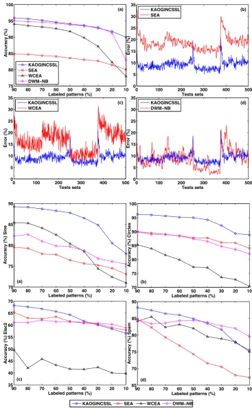
Figure3(a) shows the accuracy for the tested algorithms on the nine different experiments regarding the percentage of labeled pattern in the training sets for the SEA domain. Each experiment result shows the classification accuracy on a test set averaged by 20 runs. Figures 3(b)–(d) show the results for the experiment with data sets with 20 % of labeled patterns. The results consist of the classification error rates for every presented test set, also averaged by 20 runs. The results of each algorithm under comparison (red curves) and the results of the proposed algorithm (blue curves) are put together and shown in Figs.3(b)–(d).
Considering the experimental results displayed in Fig.3(a), as expected, all the algorithms tend to degener-ate their performance as the labeling percentage provided in the training sets decays. Notice that the proposed algo-rithm KAOGINCSSL and the DWM-NB algoalgo-rithm have performed similarly throughout all the different label per-centages domains, with exception to the experiment with 10 % of labeled patterns where the KAOGINCSSL algo-rithm presented a better performance. In fact, even when only 20 % of the training patterns are labeled, KAOGINC-SSL and DWM-NB present similar performance, differ-entiating by the fact that the proposed algorithm is much more stable, presenting the smallest variance. Regarding the WCEA algorithm, from Fig.3(a), we see that it is the algo-rithm that suffers the most as the amount of labeled patterns decreases. Again, when considering 20 % labeled set, in spite of presenting very close result for the average error percentage to the SEA algorithm performance, the WCEA algorithm presents a larger variation on error rate along the stream processing, as can be seem in Figs. 3(b)–(c). The SEA ensemble has the worst performance in this domain.
Now, consider the experiments on the other two artificial domains (Sine and Circle) and the two real domains (Elec2 and Spam), again, each with nine different realizations and classification results taken as the mean over all presented test sets averaged by 20 runs. Figure4presents the results.
Fig. 3 Experiments with the SEA domain, (a) average accuracy for nine experiments with different percentages of labeled patterns, from 10 % to 90 %; and performance comparison through the SEA presentation with 20 % labeled patterns, between the KAOGINCSSL and (b) SEA, (c) WCEA and (d) DWM-NB
Fig. 4 Experiments with nine different percentages of labeled patterns in each data set for the domains Sine, Circle, Elec2 and Spam
the other algorithms, considering all the experiment config-urations. This advantage, though, seems to decrease when real data sets are considered, which may be due to the fact that artificial domains are constructed in a controlled manner
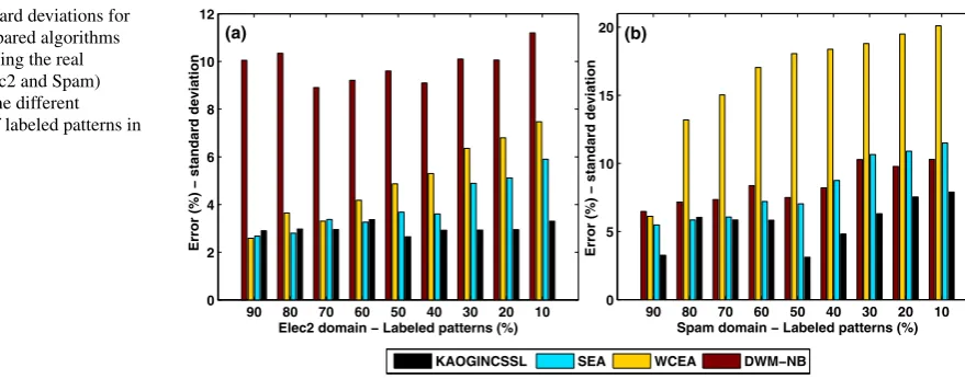
Fig. 5 Standard deviations for the four compared algorithms when processing the real domains (Elec2 and Spam) within the nine different percentage of labeled patterns in each data set
the proposed algorithm in the artificial domains can be par-tially explained due to the KAOGINCSSL ability to get rid of past concepts much faster than the ensemble algorithms used for comparison. Now, for better analyzing the real do-mains, consider also the standard deviation among the pre-sented test sets and taken from a single run to best represent a real situation. Figure5presents the standard deviation for the nine considered experiments and the four compared al-gorithms when processing the real domains Elec2 and Spam. In real applications, low variance or standard deviation is a desirable feature for a classifier, precisely the lower the standard deviation the more reliable is the classifier perfor-mance. Therefore, considering the results for the electricity domain presented in Fig.4(c); except for the WCEA algo-rithm, all the others have presented a similar performance, in special for low levels of labeling (<40 %). Here, again the proposed algorithm obtained the best performances for the experiments with more than 50 % of labeled data. Analyzing the standard deviation in Fig.5(a), it is easy to verify that the proposed algorithm presents the most reliable performance. The DWM-NB algorithm presents too higher values of stan-dard deviation indicating high fluctuation in classification performance, in spite of presenting good average accuracy. The SEA ensemble has good accuracy results and low vari-ance.
Regarding the results of the KAOGINCSSL algorithm in the Spam base shown in Fig.4(d), at a first glance, almost the same trend as in the Elec2 domain can be observed. Because it has presented best average accuracy performance for ex-periments with more than 50 % labeled patterns and average performance for the rest. In spite of that, the KAOGINC-SSL algorithm shows again the most regular performance as depicted in Fig.5(b). The DWM-NB algorithm has also per-forms well, particularly up to the point where labeled data instances fall off from least than 40 %, but with higher stan-dard deviation than the KAOGINCSSL. Thus, we can say that both KAOGINCSSL and DWM-NB algorithms perform similarly. The SEA ensemble presents the lowest average
accuracy but small standard deviation, while the WCEA in-stead of presenting near average mean accuracy also shows too high standard deviation, which discourages both to be used in this domain.
It is also important to notice that all the algorithms, which have used the KAOGSS as transduction algorithm, present good results, especially in the real domains. Therefore, we verify that the proposed transduction algorithm KAOGSS, not only can be used in association to the KAOGINCSSL algorithm, but also can be successfully used in other algo-rithms as well.
5 Conclusions
This paper has introduced a semi-supervised graph-based algorithm suitable for non-stationary streaming application, particularly when only a small portion of the acquired data presents label. Comparative results on artificial and real data sets performed on the proposed method against three well-know ensemble methods show that the proposed algorithm outperformed the compared algorithms in most of the exper-iments. Moreover, the results show that the present spread-ing label technique can be used successfully in other super-vised learning algorithms to support semi-supersuper-vised clas-sification. Future work includes testing the proposed algo-rithm with more data sets and comparing to other algoalgo-rithms with their own spreading label method, as well as comparing the accuracy of the optimal graph as a transductive method against other transductive ones.
Acknowledgements This work is supported by the Brazilian Na-tional Research Council (CNPq) and by the São Paulo State Research Foundation (FAPESP).
References
2. Belkin M, Niyogi P, Sindhwani V (2006) Manifold regularization: a geometric framework for learning from labeled and unlabeled examples. J Mach Learn Res 1:1–48
3. Bertini JR Jr, Lopes A, Motta R, Zhao L (2010) Online classifier based on the optimalK-associated network. In: Proceedings of the joint conference, III international workshop on web and text intelligence (WTI’10), pp 826–835
4. Bertini JR Jr, Zhao L, Motta R, Lopes A (2011) A nonparamet-ric classification method based onK-associated graphs. Inf Sci 181:5435–5456
5. Bornholdt S, Schuster H (eds) (2003) Handbook of graphs and networks: from the genome to the Internet, 1st edn. Wiley-VCH, Weinheim
6. Breve FA, Zhao L, Quiles M, Pedrycz W, Liu J (2011) Parti-cle competition and cooperation in networks for semi-supervised learning. IEEE Trans Knowl Data Eng. doi:10.1109/TKDE.2011. 119
7. Chapelle O, Zien A, Schölkopf B (eds) (2006) Semi-supervised learning, 1st edn. MIT Press, Cambridge
8. Chapelle O, Sindhwani V, Keerthi S (2008) Optimization tech-niques for semi-supervised support vector machines. J Mach Learn Res 9:203–233
9. Cormen T, Leiserson C, Rivest R, Stein C (2009) Introduction to algorithms, 3rd edn. MIT Press, Cambridge
10. Culp M, Michailidis G (2008) Graph-based semisupervised learn-ing. IEEE Trans Pattern Anal Mach Intell 30(1):174–179 11. Ditzler G, Polikar R (2011) Semi-supervised learning in
nonsta-tionary environments. In: Proceedings of international joint con-ference on neural networks (IJCNN’11), San Jose, CA, USA. IEEE Press, New York, pp 2741–2748
12. Erman J, Mahanti A, Arlitt M, Cohen I, Williamson C (2007) Of-fline/realtime traffic classification using semi-supervised learning. Perform Eval 64:1194–1213
13. Gama J, Medas P, Castillo G, Rodrigues P (2004) Learning with drift detection. In: Proceedings of the Brazilian symposium on ar-tificial intelligence (SBIA’04), vol 3171. Springer, Berlin, pp 286– 295
14. Giraud-Carrier C (2000) A note on the utility of incremental learn-ing. AI Commun 13(4):215–223
15. Hastie T, Tibshirani R, Friedman J (2009) The elements of sta-tistical learning: data mining, inference and prediction, 2nd edn. Springer, Berlin
16. Hettich S, Bay S (1999) The UCI KDD archive. University of California, Irvine, School of Information and Computer Sciences.
http://kdd.ics.uci.edu/
17. Kelly M, Hand D, Adams N (1999) The impact of changing populations on classifier performance. In: Proceedings of the in-ternational conference on knowledge discovery and data mining (KDD’99). ACM, New York, pp 367–371
18. Klinkenberg R, Joachims T (2000) Detecting concept drift with support vector machines. In: Proceedings of the international con-ference on machine learning (ICML’00). Morgan Kaufmann, San Mateo, pp 487–494
19. Kolter JZ, Maloof MA (2007) Dynamic weighted majority: an en-semble method for drifting concepts. J Mach Learn Res 8:2755– 2790
20. Li P, Wu X, Hu X (2010) Mining recurring concept drift with lim-ited labeled streaming data. In: JLMR: workshop and conference proceedings, vol 13, pp 241–252
21. Lopes AA, Bertini JR Jr, Motta R, Zhao L (2009) Classification based on the optimal k-associated network. In: Proceedings of the international conference on complex sciences: theory and applica-tions (COMPLEX’09). Lecture notes of the Institute for Computer Sciences, Social-Informatics and Telecommunications Engineer-ing (LNICST), vol 4. SprEngineer-inger, Berlin, pp 1167–1177
22. Masud M, Gao J, Khan L, Han J (2008) A practical approach to classify evolving data streams: training with limited amount of la-beled data. In: Proceeding of the international conference on data mining (ICDM’08)
23. Minku L, White A, Yao X (2010) The impact of diversity on online ensemble learning in the presence of concept drift. IEEE Trans Knowl Data Eng 22:730–742
24. Narasimhamurthy A, Kuncheva L (2007) A framework for gen-erating data to simulate changing environments. In: Proceed-ings of the international artificial intelligence and applications (ICAIA’07), pp 384–389
25. Quiles M, Zhao L, Alonso RL, Romero RAF (2008) Particle competition for complex network community detection. Chaos 18:033107
26. Quinlan JR (1993) C4.5 programs for machine learning, 1st edn. Morgan Kaufmann, San Mateo
27. Schaeffer S (2007) Graph clustering. Comput Sci Rev 1:27–34 28. Schlimmer J, Granger R (1986) Beyond incremental processing:
tracking concept drift. In: Proceedings of the association for the advancement of artificial intelligence (AAAI’86). AAAI Press, Menlo Park, pp 502–507
29. Street N, Kim Y (2001) A streaming ensemble algorithm (SEA) for large-scale classification. In: Proc int’l conf knowledge discov-ery and data mining (KDD’01). ACM, New York, pp 377–382 30. Sung J, Kim D (2009) Adaptive active appearance model with
in-cremental learning. Pattern Recognit Lett 30:359–367
31. Syed N, Liu H, Sung K (1999) Handling concept drift in incremen-tal learning with support vector machines. In: Proceedings of the international conference on knowledge discovery and data mining (KDD’99), pp 272–276
32. von Luxburg U (2007) A tutorial on spectral clustering. Stat Com-put 17:395–416
33. Wang H, Fan W, Yu P, Han J (2003) Mining concept-drifting data streams using ensemble classifiers. In: Proc international confer-ence on knowledge discovery and data mining (KDD’03), pp 226– 235
34. Widmer G, Kubat M (1996) Learning in the presence of concept drift and hidden contexts. Mach Learn 23(1):69–101
35. Yang C, Zhou J (2008) Non-stationary data sequence classification using online class priors estimation. Pattern Recognit 41:2656– 2664
36. Yu Y, Guo S, Lan S, Ban T (2008) Anomaly intrusion detection for evolving data stream based on semi-supervised learning. In: Proceedings of the international conference on advances in neuro-information processing (NIPS’08), pp 571–578
37. Zhang P, Zhu X, Guo L (2009) Mining data streams with labeled and unlabeled training examples. In: Proceedings of the ninth IEEE international conference on data mining (ICDM’09). IEEE Press, New York, pp 627–636
38. Zhu X (2008) Semi-supervised learning literature survey. Tech Rep 1530, Computer-Science, University of Wisconsin-Madison 39. Zhu X (2005) Semi-supervised learning with graphs. Tech Rep