https://doi.org/10.5194/npg-25-145-2018 © Author(s) 2018. This work is distributed under the Creative Commons Attribution 4.0 License.
A general theory on frequency and time–frequency analysis of
irregularly sampled time series based on projection methods –
Part 1: Frequency analysis
Guillaume Lenoir1and Michel Crucifix1,2
1Georges Lemaître Centre for Earth and Climate Research, Earth and Life Institute, Université catholique de Louvain, 1348, Louvain-la-Neuve, Belgium
2Belgian National Fund of Scientific Research, rue d’Egmont, 5, 1000 Brussels, Belgium Correspondence:Guillaume Lenoir ([email protected])
Received: 16 June 2017 – Discussion started: 4 July 2017
Revised: 4 December 2017 – Accepted: 6 December 2017 – Published: 5 March 2018
Abstract.We develop a general framework for the frequency analysis of irregularly sampled time series. It is based on the Lomb–Scargle periodogram, but extended to algebraic op-erators accounting for the presence of a polynomial trend in the model for the data, in addition to a periodic com-ponent and a background noise. Special care is devoted to the correlation between the trend and the periodic compo-nent. This new periodogram is then cast into the Welch over-lapping segment averaging (WOSA) method in order to re-duce its variance. We also design a test of significance for the WOSA periodogram, against the background noise. The model for the background noise is a stationary Gaussian continuous autoregressive-moving-average (CARMA) pro-cess, more general than the classical Gaussian white or red noise processes. CARMA parameters are estimated follow-ing a Bayesian framework. We provide algorithms that com-pute the confidence levels for the WOSA periodogram and fully take into account the uncertainty in the CARMA noise parameters. Alternatively, a theory using point estimates of CARMA parameters provides analytical confidence levels for the WOSA periodogram, which are more accurate than Markov chain Monte Carlo (MCMC) confidence levels and, below some threshold for the number of data points, less costly in computing time. We then estimate the amplitude of the periodic component with least-squares methods, and derive an approximate proportionality between the squared amplitude and the periodogram. This proportionality leads to a new extension for the periodogram: the weighted WOSA periodogram, which we recommend for most frequency anal-yses with irregularly sampled data. The estimated signal
am-plitude also permits filtering in a frequency band. Our re-sults generalise and unify methods developed in the fields of geosciences, engineering, astronomy and astrophysics. They also constitute the starting point for an extension to the con-tinuous wavelet transform developed in a companion article (Lenoir and Crucifix, 2018). All the methods presented in this paper are available to the reader in the Python package WAVEPAL.
1 Introduction
In many areas of geophysics, one has to deal with irregularly sampled time series. However, most state-of-the-art tools for the frequency analysis are designed to work with reg-ularly sampled data. Classical methods include the discrete Fourier transform (DFT), jointly with the Welch overlapping segment averaging (WOSA) method, developed by Welch (1967), or the multitaper method, designed in Thomson (1982) and Riedel and Sidorenko (1995). Given the excel-lent results they provide, it is tempting to interpolate the data and simply apply these techniques. Unfortunately, interpola-tion may seriously affect the analysis with unpredictable con-sequences for the scientific interpretation (Mudelsee, 2010, p. 224).
as-tronomy, e.g. in Mortier et al. (2015), Vio et al. (2010), or Zechmeister and Kürster (2009), and in geophysics, e.g. in Schulz and Stattegger (1997), Schulz and Mudelsee (2002), Mudelsee et al. (2009), Pardo Igúzquiza and Rodríguez Tovar (2012), or Rehfeld et al. (2011). More specifically, in climate and paleoclimate, the time series are often very noisy, exhibit a trend, and potentially carry a wide range of periodic com-ponents (see e.g. Fig. 6). Considering all these properties, we design in this work an operator for the frequency analy-sis generalising the LS periodogram. The latter was built to analyse data which can be modelled as a periodic component plus noise. Since the periodic component may not necessar-ily oscillate around zero, Ferraz-Mello (1981) and Heck et al. (1985) extended the LS periodogram, proposing an operator that is suitable to analyse data which can be modelled as a periodic component plus a constant trend plus noise. Their operator is designed to take into account the correlation be-tween the constant trend and the periodic component, and is now a classic tool for analysing astronomical irregularly spaced time series. In climate and paleoclimate, the periodic component may oscillate around a more complex trend than just a constant. This is why, in this work, we extend the previ-ous result by proposing an operator that is suitable to analyse data which can be modelled as a periodic component plus a polynomial trend plus noise. Our operator is also designed to take into account the correlation between the trend and the periodic component. Our extended LS periodogram is, however, not sufficient to deal with very noisy data sets, and it also exhibits spectral leakage, like the DFT. In the world of regularly sampled and very noisy time series, smoothing techniques can be applied to reduce the variance of the pe-riodogram, after tapering the time series in order to allevi-ate spectral leakage (see Harris, 1978). One of them is the WOSA method (Welch, 1967), which consists of segmenting the time series into overlapping segments, tapering them, tak-ing the periodogram on each segment, and finally taktak-ing the average of all the periodograms. This technique was trans-ferred to the world of irregularly sampled time series in the work of Schulz and Stattegger (1997), where they apply the classical LS periodogram to each tapered segment, and take the average. In this article, we generalise their work by ap-plying the tapered WOSA method to our extended LS peri-odogram. Moreover, we show that it is preferable to weight the periodogram of each WOSA segment before taking the average in order to get a reliable representation of the squared amplitude of the periodic component. This leads us to define theweighted WOSA periodogram, which we recommend for most frequency analyses.
The periodogram is often accompanied by a test of signif-icance for the spectral peaks, which relies on the choice of an additive background noise. Two traditional background noises are used in practice. The first one is the Gaussian white noise, which has a flat power spectral density, and which is a common choice with astronomical data sets, e.g. in Scargle (1982) or Heck et al. (1985). The second one
is the Gaussian red noise or Ornstein–Uhlenbeck process, for which the power spectral density is a Lorentzian func-tion centred at frequency zero, and which is a common choice with (palaeo-)climate time series, e.g. those in Schulz and Mudelsee (2002) or Ghil et al. (2002). Arguments in favour of a Gaussian red noise as the background stochas-tic process for climate time series are given in Hasselmann’s influential paper (Hasselmann, 1976). Other background noises are also found in geophysics, often under the form of an autoregressive-moving-average (ARMA) process (see Mudelsee, 2010, p. 60, for an extensive list). In this work, we consider a general class of background noises, which are the continuous autoregressive-moving-average (CARMA) pro-cesses, defined in Sect. 3.2. A CARMA(p, q) process is the extension of an ARMA(p, q) process to a continuous time (Brockwell and Davis, 2016, Sect. 11.5). Gaussian white noise and Gaussian red noise are particular cases of a Gaus-sian CARMA process, i.e. they are a CARMA(0,0) process and a CARMA(1,0) process, respectively. Recent advances now allow for accurate estimation of the parameters of an ir-regularly sampled CARMA process from one of its samples (see Kelly et al., 2014).
Estimating the percentiles of the distribution of the weighted WOSA periodogram of an irregularly sampled CARMA process is the core of this paper. This gives the con-fidence levels for performing tests of significance at every frequency, i.e. test if the null hypothesis – the time series is a purely stochastic CARMA process – can be rejected (with some percentage of confidence) or not. We aim at developing a very general approach. Let us enumerate some key points.
1. Estimation of CARMA parameters is performed in a Bayesian framework and relies on state-of-the-art algo-rithms provided by Kelly et al. (2014). In the special case of a white noise, we provide an analytical solution. 2. Based on 1, we provide confidence levels computed with Markov chain Monte Carlo (MCMC) methods, that fully take into account the uncertainty of the parameters of the CARMA process, because we work with a distri-butionof values for the CARMA parameters instead of a unique set of values.
3. Alternatively to 2, if we opt for the traditional choice of a unique set of values for the parameters of the CARMA background noise, we develop a theory providing ana-lyticalconfidence levels. Compared to a MCMC-based approach, the analytical method is more accurate and, if the number of data points is not too high, quicker to compute, especially at high confidence levels, e.g. 99 or 99.9 %. Computing high levels of confidence is re-quired in some studies, for example in paleoceanogra-phy (Kemp, 2016).
ex-tending the traditional 50 % overlapping choice (Schulz and Stattegger, 1997; Schulz and Mudelsee, 2002). 5. Under the case of a white noise background, without
WOSA segmentation and without tapering, we define theF periodogramas an alternative to the periodogram. It has the advantage of not requiring any parameter to be estimated.
Finally, we note that spectral power and estimated squared amplitude are no longer the same thing if the time series is irregularly sampled. Both quantities may be of physical interest. We estimate the amplitude of the periodic com-ponent with least-squares methods, and derive an approxi-mate proportionality between the squared amplitude and the periodogram, from which we deduce the weights for the weighted WOSA periodogram. The estimated signal ampli-tude also gives access to filtering in a frequency band.
The paper is organised as follows. In Sect. 2, we introduce the notations and recall some basics of algebra. In Sect. 3, we define the model for the data and write the background noise term into a suitable mathematical form. Section 4 starts with some reminders about the Lomb–Scargle periodogram and then extends it to take into account the trend, and a second ex-tension deals with the WOSA tapered case. In Sect. 5, we re-mind the reader that significance testing is nothing but a sta-tistical hypothesis testing. Under the null hypothesis, we esti-mate the parameters of the CARMA process and estiesti-mate the distribution of the WOSA periodogram, either with Monte Carlo methods or analytically. In the case of a white noise background, we define the F periodogram as an alternative to the periodogram. Section 6 aims at computing the amplitude of the periodic component of the signal, and the difference between the squared amplitude and the periodogram is ex-plained. Sections 7 and 8 are based on the results of Sect. 6. There, we propose a third extension for the LS periodogram and show how to perform filtering. Section 9 presents an ex-ample of analysis on a palaeoceanographic time series. Fi-nally, a Python package named WAVEPAL is available to the reader and is presented in Sect. 10.
2 Notations and mathematical background 2.1 Notations
Let us introduce the notations for the time series. The mea-surementsX1, X2, . . ., XN are done at the timest1, t2, . . ., tN
respectively, and we assume there is no error in the measure-ments or in the times. They are cast into vectors belonging to
RN:
|ti =
t1
t2
.. . tN
and |Xi =
X1
X2
.. . XN
. (1)
We use here the bra–ket notation, which is common in physics. InRN, the transpose of|aiisha|, i.e.ha|0= |ai, and
inCN,ha|is the conjugate transpose of|ai, i.e.ha|∗= |ai. The inner product of|aiand|biisha|bi.
– LetAbe a(m, n)matrix andBbe a(n, m)matrix. If Ais real,A0denotes its transpose, and ifAis complex, A∗ denotes its conjugate transpose. The trace ofABis denoted by tr(AB)and we have tr(AB)=tr(BA). – Let|Yi be a vector inRN andAbe a(M, N )matrix.
The notationsA|Yiand|AYirefer to the same vector. – We use the terminologyGaussian white noiseor simply
white noisefor a (multivariate) Gaussian random vari-able with constant mean and covariance matrixσ2I. – |Zi always denotes a standard multivariate Gaussian
white noise, i.e.
|Zi=d N(0,I), (2)
where=d means “is equal in distribution” and Iis the identity matrix.
– A sequence of independent and identically distributed random variables is denoted by “iid”.
2.2 Orthogonal projections inRN
The orthogonal projection on a vector space spanned by the
mlinearly independent vectors|a1i, ...,|amiinRNfor some m∈N0(m≤N) is
Psp{|a1i,...,|ami}=V(V
0V)−1V0, (3)
where sp{|a1i, . . .,|ami}is the closed span of those m
vec-tors, i.e. the set of all the linear combinations between them. Vis a(N, m)matrix defined by
V=
| |
|a1i . . . |ami
| |
. (4)
Like for any orthogonal projection, we have the following equalities:
Psp{|a1i,...,|ami}=P 0
sp{|a1i,...,|ami}=P
2
sp{|a1i,...,|ami}. (5)
Themlinearly independent vectors|a1i, ...,|amimay be
or-thonormalised by a Gram–Schmidt procedure, leading tom
orthonormal vectors|b1i, ...,|bmi, and the orthogonal
pro-jection may then be rewritten as
Psp{|a1i,...,|ami}=Psp{|b1i,...,|bmi}= m
X
k=1
|bkihbk|. (6)
Under that form, we see that the above projection has m
Let |c1i, ..., |cqi be q linearly independent vectors
in RN, with q≤m, and such that sp{|c
1i, . . .,|cqi} ⊆
sp{|a1i, . . .,|ami}. Then (Psp{|a1i,...,|ami}−Psp{|c1i,...,|cqi})
is an orthogonal projection on sp{|c1i, . . .,|cqi} ∩
sp{|a1i, . . .,|ami}⊥, and
Psp{|a1i,...,|ami}Psp{|c1i,...,|cqi}
=Psp{|c1i,...,|cqi}Psp{|a1i,...,|ami}
=Psp{|c1i,...,|cqi}. (7)
Moreover, for any vector|Yi ∈RN, we have ||(Psp{|a1i,...,|ami}−Psp{|c1i,...,|cqi})|Yi||
2 = ||Psp{|a1i,...,|ami}|Yi||
2− ||P
sp{|c1i,...,|cqi}|Yi||
2. (8) We recommend the book of Brockwell and Davis (1991) for more details.
2.3 Quantifying the irregularity of the sampling The biggest time step for whicht1, ...,tN are a subsample
of a regularly sampled time series is the greatest common divisor1(GCD) of all the time steps of|ti. In formulas,
1tGCD=GCD(1t1, . . ., 1tN−1) , (9) where
1tk=tk+1−tk ∀k∈ {1, . . ., N−1}, (10)
and
∀k∈ {1, . . ., N},∃m∈Zs.t.tk=m1tGCD, (11) whereZdenotes the space of integer numbers. Quantifying
the irregularity of the sampling is then straightforward. We define
rt =100
(N−1)1tGCD
tN−t1
. (12)
This ratio is between 0 and 100 %, the latter value being reached with regularly sampled time series.
3 The model for the data 3.1 Definition
A suitable and general enough model to analyse the period-icity at frequencyf=
2π is
|Xi = |Trendi +Eωcos(|ti +φω)+ |Noisei
= |Trendi +Aω|ci +Bω|si + |Noisei, (13)
1The GCD is usually defined on the integers, but we can extend
it to rational numbers. In practice,t1, ...,tN come from measure-ments with a finite precision and are thus rational numbers.
withAω=Eωcos(φω),Bω= −Eωsin(φω), andE2ω=A2ω+
Bω2. The terms |ci and |si are defined
component-wise, i.e.|ci =cos(|ti)= [cos(t1), . . .,cos(tN)]0 and
|si =sin(|ti)= [sin(t1), . . .,sin(tN)]0. We have added
the subscriptωto differentiate between the probed frequency,
ω, and the data frequency,. Indeed, the periodogram (de-fined in Sect. 4), the amplitude periodogram (Sect. 6) and the weighted WOSA periodogram (Sect. 7) do not necessarily probe the signal at its true frequency.
3.2 The background noise
3.2.1 Definition of a CARMA process
We follow here the definitions and conventions of Kelly et al. (2014), and technical details can be found in Brockwell and Davis (2016, Sect. 11.5).
The background noise term, |Noisei, considered in this paper is a zero-mean stationary Gaussian CARMA process sampled at the times of |ti. As explained in the follow-ing, it generalises traditional background noises used in geo-physics.
A CARMA(p, q) process is simply the extension of an ARMA(p, q) process to a continuous time2. A zero-mean CARMA(p, q) processy(t )is the solution of the following stochastic differential equation:
dpy(t )
dtp +αp−1
dp−1y(t )
dtp−1 +. . .+α0y(t ) =βq
dq(t )
dtq +βq−1
dq−1(t )
dtq−1 +. . .+(t ), (14) where (t ) is a continuous-time white noise process with zero mean and varianceσ2. It is defined from the standard Brownian motionB(t )through the following formula:
σdB(t )=(t )dt. (15)
The parametersα0, ... ,αp−1 are the autoregressive coeffi-cients, and the parametersβ1, ..., βq are the moving
aver-age coefficients;αp=β0=1 by definition. Whenp >0, the process is stationary only ifq < pand the rootsr1, . . ., rpof
p
X
k=0
αkzk=0 (16)
have negative real parts. Strictly speaking, the derivatives of the Brownian motionddkBt ,k >0, do not exist, and we there-fore interpret Eq. (14) as being equivalent to the following measurement and state equations:
y(t )= hb|w(t )i, (17)
and
d|w(t )i =A|w(t )idt+dB(t )|ei, (18)
2A CARMA(p, q) process sampled at the times of an infinite
where|bi = [β0, β1, . . ., βq,0, . . .,0]0is a vector of lengthp,
|ei = [0,0, . . .,0, σ]0, and
A=
0 1 0 . . . 0
0 0 1 . . . 0
..
. ... ... . .. ...
0 0 0 . . . 1
−α0 −α1 −α2 . . . −αp−1
. (19)
Equation (18) is nothing else but an Itô differential equation for the state vector|w(t )i.
In practice, only CARMA processes of low order are use-ful in our framework, typically,(p, q)=(0,0),(1,0),(2,0),
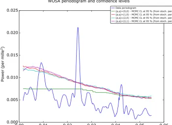
(2,1), since at a higher order, they often exhibit dominant spectral peaks (see Kelly et al., 2014), which is not what we want as a model for the spectral background. Indeed, on the basis of our model, Eq. (13), it is desirable that the spec-tral peaks come from the deterministic cosine and sine com-ponents. We now consider two useful particular cases of a CARMA process before analysing the general case.
3.2.2 Gaussian white noise
Whenp=0 andq=0, the process reduces to a white noise, normally distributed with zero mean and variance σ2. The |Noiseiterm in Eq. (13) is then simply
|Noisei =σ|Zi =K|Zi, (20)
withK=σI.
3.2.3 Gaussian red noise
When p=1 andq=0, the CARMA(1,0) or CAR(1) pro-cess is an Ornstein–Uhlenbeck propro-cess or red noise (Uhlen-beck and Ornstein, 1930), which is quite of interest in geo-physical and other applications (Mudelsee, 2010). Since we work with a discrete time series, it is necessary to find the solution of Eq. (14) at t1, ..., tN. This is done by
integrat-ing that equation between consecutive times, i.e. fromti−1to
ti ∀i∈ {2, . . ., N}. The components of the|Noiseivector are
then as follows:
y(t1)=d N
0,σ
2 2α
,
y(ti)=ρiy(ti−1)+ηi, ∀i∈ {2, . . ., N}, (21)
where
ρi=exp(−α(ti−ti−1)) and
ηi d
=N
0,σ
2 2α(1−ρ
2
i)
. (22)
See Robinson (1977) and Brockwell and Davis (2016, p. 343) for more details. The requirement on stationarity, Eq. (16), imposesα >0. The generated time series has a con-stant mean equal to zero and a concon-stant variance equal to σ2α2.
The|Noiseiterm in Eq. (13) can also be written under a ma-trix form:
|Noisei =K|Zi, (23)
whereKis a(N, N )lower triangular matrix whose elements are
Ki,j =
s σ2
2α q
1−ρj2exp −α(ti−tj)
, ∀j ≤i, (24) where we define ρ1=0. This matrix form is used in Sect. 5.3.3.
Note that, if the time series is regularly sampled,ρ is a constant and Eq. (21) becomes the equation of a finite-length AR(1) process, which is stationary sinceα >0 impliesρ <
1.
3.2.4 The general Gaussian CARMA noise
The solution of Eq. (14) at the timetn(n=2, . . ., N), that we
denote byyn, is
yn= hb|wni,
where|wni =exp(A(tn−tn−1))|wn−1i + |ηni, (25)
where|ηni follows a multivariate normal distribution with
zero mean and covariance matrixCngiven by
Cn= tn−tn−1
Z
0
dtexp(At )|eihe|exp(A0t ). (26)
The above formula requires the computation of matrix expo-nentials and numerical integration. This can be avoided by diagonalising matrixA, with A=UDU−1.Dis a diagonal matrix with diagonal elements given by the roots of Eq. (16):
Dkk=rk, ∀k∈1, . . ., p, (27)
andUis a Vandermonde matrix, with
Ulk=rkl−1 ∀l, k∈1, . . ., p. (28)
Now, by defining|
e
wni =U−1|wni, we get
yn= hb|U|weni, (29a)
where|
e
wni =3n|wen−1i + |eηni. (29b)
The matrix exponential exp(A(tn−tn−1)) has been trans-formed into3n=U−1exp(A(tn−tn−1))U, which is simply a diagonal matrix with elements3nkk=exp(rk(tn−tn−1)). The covariance matrix of|
eηni, that we write6n, also takes a
relatively simple form:
6nkl= −σ2 κkκ
∗
l
rk+rl∗
∀k, l∈ {1, . . ., p}, (30) which is a Hermitian matrix, and where|κiis the last column of U−1. The initial conditiony
1is determined by imposing stationarity, which is fulfilled only if|w1ihas a zero mean and a covariance matrixVwhose elements are
Vkl= −σ2 p
X
m=1
rmk−1(−rm)l−1
2Re{rm}Qps=1,s6=m(rs−rm)(rs∗+rm)
,
∀k, l∈ {1, . . ., p}. (31)
Stationarity implies that the processy(t )has a zero mean and variance hb|V|bi∀t. All the above formulas and how to get them can be found in Kelly et al. (2014), Jones and Ackerson (1990) and Brockwell and Davis (2016, Sect. 11.5.2).
Generation of a CARMA(p, q)process can be performed with the Kalman filter since Eqs. (29b) and (29a) are nothing but the state and measurement equations, respectively (see Kelly et al., 2014, for more details). Alternatively,|yican be written under a matrix form as in Eq. (23). Matrix formalism is useful in Sect. 5.3.3. Let us start with Eq. (29b):
|
e
wni =3n|wen−1i +U
−1|η
ni. (32)
The covariance matrix of|ηni,Cn=U6U∗, is of course real
symmetric and positive semi-definite. We thus have the fol-lowing Schur decomposition:
Cn=QnQ0n, (33)
whereQnis a real matrix. Consequently,
|
e
wni =3n|wen−1i +U
−1Q
n|ni
=3n3n−1|wen−2i +3nU
−1Q
n−1|n−1i +U−1Qn|ni
=. . .
=
n
X
i=2
n
Y
l=i+1
3l
!
U−1Qi|ii + n
Y
l=2
3l|we1i, (34)
where|1i, ...,|niare iid standard Gaussian white noises.
The product of the3’s can be simplified. Its diagonal ele-ments are as follows:
(Yin)jj:= n
Y
l=i+1
3l !
jj
=exp rj(tn−ti)
. (35)
As stated above, |w1i follows a multivariate normal distri-bution with zero mean and covariance matrixV. We can use again the Schur decomposition to writeV=WW0, whereW is a real matrix, yielding
|
e wni =
n
X
i=2
YinU−1Qi|ii +Y1nU−1W|1i
=
n
X
i=1
Pin|ii, (36)
withP1n=Y1nU−1WandPin=YinU−1Qi for i >1. The
CARMA process at timetnis then given by
yn= hb|U|weni
=
n
X
i=1
hb|U|Pin|ii. (37)
Finally, the|Noiseiterm in Eq. (13) is |Noisei = |yi
=
hb|U|P11 h0| . . . h0| hb|U|P12 hb|U|P22 h0| . . . h0|
. .. . ..
hb|U|P1N hb|U|P2N . . . hb|U|PN N
|1i |2i . . . |Ni
=K|Zi, (38)
whereKis a(N, N×p) real matrix and|Zi has a length
N×p. MatrixKis triangular ifp=1, which is the particular case treated in Sect. 3.2.3.
3.3 The trend
The model for the trend must be as general as possible and compatible with a formalism based on orthogonal projections (see Sect. 4). This is the reason we choose a polynomial trend of some degreem:
|Trendi =
m
X
k=0
γk|tki, where|tki = [t1k, . . ., t
k N]
0
, (39)
where|tkiis defined componentwise, i.e.|tki = [t1k, . . ., tNk]0. Whether or not to consider the presence of a trend in the model for the data is left to the user, given that we can al-ways interpret a polynomial trend of low order as a very low-frequency oscillation.
4 Periodogram and relatives 4.1 Lomb–Scargle periodogram
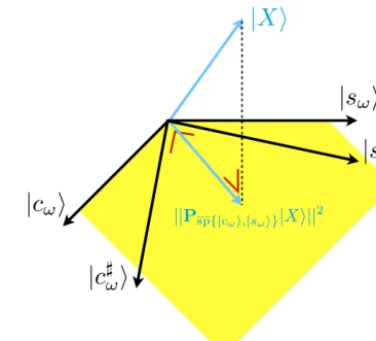
Consider the orthogonal projection of the data|Xi onto the vector space spanned by the vectors cosine and sine, defined by|cωi =cos(ω|ti)and|sωi =sin(ω|ti). The periodogram
at the frequencyf = ω
2π is defined as the squared norm of
that projection:
||Psp{|cωi,|sωi}|Xi||2. (40)
When the time series is regularly sampled with a constant time step 1t, and if we only consider the Fourier angular frequencies,ωk=N 1t2π k (k=0, ..., N−1), the periodogram
Now, rescale|cωiand|sωisuch that they are orthonormal.
This can be done by defining |cω]i = cos(ω|ti −βω)
q
6iN=1cos2(ωt
i−βω)
,
|s]ωi = sin(ω|ti −βω)
q
6iN=1sin2(ωti−βω)
, (41)
whereβωis the solution of
tan(2βω)=
6Ni=1sin(2ωti)
6iN=1cos(2ωti)
. (42)
The spanned vector space naturally remains unchanged (see Fig. 1). These formulas are nothing but the Lomb–Scargle formulas (Scargle, 1982, Eq. 10). The periodogram is now ||Psp{|cωi,|sωi}|Xi||2= hc]ω|Xi2+ hsω]|Xi2. (43)
Note that, for any signal|Xi ∈RN, 0≤ ||Psp{|cωi,|sωi}|Xi||
2
hX|Xi ≤1, (44)
and this is equal to 1 if|Xi =A|cωi +B|sωi.
Some properties of the LS periodogram are presented in Appendix A. Here and for the rest of the article, the fre-quencyf =ω/2πis considered as a continuous variable. 4.2 Periodogram and mean
The LS periodogram applies well to data which can be mod-elled as
|Xi =Aω|ci +Bω|si + |Noisei. (45)
However, the periodic components may not necessarily os-cillate around zero, and a better model is
|Xi =µ|t0i +Aω|ci +Bω|si + |Noisei, (46)
where|t0i = [1,1, . . .,1]0. Subtracting the average of the data is then often done before applying the LS periodogram. But that mere operation implicitly assumes that ht0|ci =
ht0|si =0, which is not necessarily the case. In other words,
the data average is not necessarily equal to µ, the process mean. Figure 2a illustrates that fact. Note that this discrep-ancy occurs in regularly sampled data as well, at non-Fourier frequencies, i.e. whenN 1t is not a multiple of the probing period. See Fig. 2b.
In order to deal with the mean in a suitable way, we define the periodogram as
||(Psp{|t0i,|cωi,|sωi}−Psp{|t0i})|Xi||2. (47)
Formula (47) is taken from Brockwell and Davis (1991), Ferraz-Mello (1981) or Heck et al. (1985); equivalence be-tween them is shown in Appendix B. [Psp{|t0i,|cωi,|sωi}−
Figure 1. Schematic view of the linear rescaling inRN leading to the Lomb–Scargle formulas. In yellow is drawn a subset of sp{|cωi,|sωi}. A span is invariant under linear combinations of its vectors. The dashed line corresponds to the minimal Euclidean dis-tance between the data|Xiand sp{|cωi,|sωi}.
0 20 40 60 80 100
0.0 0.5 1.0 1.5 2.0
(a)
0 20 40 60 80 100
Time 0.0
0.5 1.0 1.5 2.0
(b)
Figure 2.Signal average and sampling.(a)The continuous signal is in dashed blue and it is irregularly sampled at red dots. The continu-ous signal oscillates around 1 (blue line), which does not correspond to the average of the sampled signal (red line).(b)Same as panel(a)
with a regularly sampled signal.
Psp{|t0i}] is also an orthogonal projection. A simple
exam-ple will justify the princiexam-ple. Consider the following purely deterministic mono-periodic signal withNdata points: |Yi =µ|t0i +A|cωi +B|sωi =V3|8i, (48) with
V3=
| | |
|t0i |cωi |sωi
| | |
and
|8i =
µ A B
. (50)
The projection atωis
Psp{|t0i,|cωi,|sωi}−Psp{|t0i}
|Yi
=I−Psp{|t0i}
Psp{|t0i,|cωi,|sωi}|Yi
=I−Psp{|t0i}
V3|8i = |Yi −Psp{|t0i}|Yi
=A|cωi +B|sωi −
ht0|cωi
ht0|t0iA|t
0i −ht0|sωi
ht0|t0iB|t
0i. (51)
We see that it is invariant with respect toµ, and we find back the signal minus its average. We thus have
||(Psp{|t0i,|cωi,|sωi}−Psp{|t0i})|Yi||
2=NVar(|Yi), (52)
where Var(|Yi)=PN
i=1Y2i
/N−PN
i=1Yi
2
/N2. This is a result similar to what we get with regularly sampled data and the DFT3.
Now, we do a Gram–Schmidt orthonormalisation like in Ferraz-Mello (1981) in order to simplify Formula (47). To this end, we define the three orthonormal vectors |h0i = |t0i/|||t0i||,|h1iand|h2isatisfying
sp{|t0i,|cωi,|sωi} =sp{|h0i,|h1i,|h2i}. (53) Consequently,
Psp{|t0i,|cωi,|sωi}−Psp{|t0i}= |h1ihh1| + |h2ihh2|, (54) and
||Psp{|t0i,|cωi,|sωi}−Psp{|t0i}
|Xi||2
= hh1|Xi2+ hh2|Xi2. (55) Note that, for any signal|Xi ∈RN, we have
≤
||Psp{|t0i,|cωi,|sωi}−Psp{|t0i}
|Xi||2
NVar(|Xi) ≤1, (56)
and this is equal to 1 for a signal given by |Xi =µ|t0i +
A|cωi +B|sωi.
3If we have|Yi =µ|t0i +A|e
ωi, where|eωi =exp(i2π ω|ti)
and ω is a Fourier frequency, then ||DFTω(|Yi)||2=
||Psp{|eωi}|Yi||
2=N||A||2=NVar(|Yi). Var is here the
bi-ased variance, which is defined as the squared norm of the signal minus its average value, and divided byN.
4.3 Periodogram and a polynomial trend
If we want to work with the full model, Eq. (13), which has a polynomial trend of degreem, we can naturally extend the result of Sect. 4.2 and work with
||Psp{|t0i,|t1i,...,|tmi,|cωi,|sωi}−Psp{|t0i,|t1i,...,|tmi}
|Xi||2 = hhm+1|Xi2+ hhm+2|Xi2, (57) where |hm+1i and |hm+2i are determined from a Gram– Schmidt orthonormalisation starting with the orthonormali-sation of|t0i, ...,|tmi.
It may happen that, for largem, the correlation matrix in the formula of orthogonal projection is singular. In that case, two options, less optimal, are possible: reduce the degreem, or perform the detrending before the spectral analysis, for example with a moving average.
Similarly to Sect. 4.2, we have, for any signal|Xi ∈RN,
0≤ ||
Psp{|t0i,|t1i,...,|tmi,|cωi,|sωi}−Psp{|t0i,|t1i,...,|tmi}
|Xi||2
|||Xi −Psp{|t0i,...,|tmi}|Xi||2
≤1, (58) and this is equal to 1 for a signal given by |Xi =
Pm
k=0γk|tki+A|cωi+B|sωi. Finally, we have a result similar
to Eq. (51), in the sense that the projection given in Eq. (57) is invariant with respect to the parameters of the trend (but it naturally depends on the choice of the degreem).
4.4 Tapering the periodogram
A finite-length signal can be seen as an infinite-length sig-nal multiplied by a rectangular window. This implies, among other things, that a mono-periodic signal will have a peri-odogram characterised by a peak of finite width, possibly with large side lobes, instead of a Dirac delta function. This is calledspectral leakage.
The phenomenon has been deeply studied in the case of regularly sampled data. Leakage may be controlled by choos-ing alternatives to the default rectangular window. This is calledwindowingortapering(see Harris, 1978, for an exten-sive list of windows). They all share the property of vanishing at the borders of the time series.
In the case of irregularly sampled data, building windows for controlling the leakage is a much more challenging task. Even with the default rectangular window, leakage is very ir-regular and is data and frequency dependent, due to the long-range correlations in frequency between the vectors on which we do the projection. To our knowledge, no general and sta-ble solution for that issue is availasta-ble in the literature. We thus recommend using the default rectangular window, i.e. do no tapering, ifrt, defined in Eq. (12), is small, and use
simple windows, like the sin2 or the Gaussian window, for moderately irregularly sampled data (rt greater than 80 or
90 %). With tapering, Formula (57) becomes ||Psp{|t0i,|t1i,...,|tmi,|Gcωi,|Gsωi}−Psp{|t0i,|t1i,...,|tmi}
whereGis a frequency-independent diagonal matrix, which is used to weight the sine and cosine vectors. For example, with a sin2window, also called Hanning window, we have
Gkk=sin2
π (tk−t1)
tN−t1
∀k∈ {1, . . ., N}. (60)
4.5 Smoothing the periodogram with the WOSA method
4.5.1 The consistency problem
Besides spectral leakage, another issue with the periodogram is consistency. Indeed, for regularly sampled time series, the periodogram is known not to be a consistent estimator of the true spectrum as the number of data points tends to in-finity (see Brockwell and Davis, 1991, chap. 10). Another view of the problem is that the periodogram remains very noisy regardless of the number of data points we have at our disposal. Smoothing procedures are therefore applied to reduce the variance of the periodogram. The drawback of any smoothing procedure is naturally a decrease of the fre-quency resolution. Among the smoothing methods available in the literature, two are traditionally used: multitaper meth-ods (MTMs), developed by Thomson (1982) and Riedel and Sidorenko (1995), and the Welch overlapping segment aver-aging (WOSA) method (Welch, 1967). See Walden (2000) for a unified view.
Multitaper methods are certainly not generalisable to the case of irregularly sampled data, except in very specific cases that are not of interest in geophysics, like in Bronez (1988), which deals with band-limited signals, useful in the field of the telecommunications, or Fodor and Stark (2000), which considers regularly sampled time series with some gaps, use-ful for time series with a ratio rt, defined in Eq. (12), close
to 100. We will then use the WOSA method applied to the LS periodogram, like in Schulz and Stattegger (1997) and Schulz and Mudelsee (2002), or to its relatives (Formulas 47, 57, or the most general 59).
4.5.2 Principle of the WOSA method Trendless time series
The time series is divided into overlapping segments. The ta-pered LS periodogram is computed on every segment, and the WOSA periodogram is the average of all these tapered periodograms. This technique relies on the fact that the sig-nal is stationary, as always in spectral asig-nalysis4. The length of the segments and the overlapping factor need to be cho-sen depending on how much we want to reduce the variance of the noise. As a general rule, shortening the segments will 4Basically, thespectrumcannot be defined without that
hypoth-esis. See the Wiener–Khinchin theorem, e.g. in Priestley (1981, chap. 4)
decrease the frequency resolution. Consequently, there is al-ways a trade-off between the frequency resolution and the variance reduction.
For regularly sampled data, each segment of fixed length has the same number of data points. In the irregularly sam-pled case, it is not the case any more and we have two op-tions.
1. Take segments with a fixed number of points and thus a variable length. In the non-tapered case, the peri-odogram on each segment provides deterministic peaks (coming from the deterministic sine–cosine compo-nents) with more or less the same height. But variable length segments will give deterministic peaks of vari-able width.
2. Take segments of fixed length but with a variable num-ber of data points. The periodogram on each segment provides deterministic peaks with more or less the same width, except if there is a big gap at the beginning or at the end of the segment, such that its effective length is reduced. But they will have variable height since the number of data points is not constant.
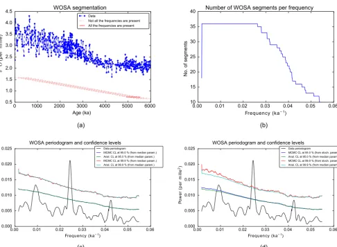
We judge it is better to have peaks with similar width on each segment when averaging the periodograms in a frequency band. Consequently, we recommend the second option. An example of WOSA segmentation is shown in Fig. 8a. Time series with a trend
The only difference with the previous case is that, for each segment, we consider the projection on|t0i, ...,|tmijointly with the tapered cosine and sine components. Formula (59) is applied to each segment with|Gcωi and|Gsωi localised
on the WOSA segment, but|t0i, ...,|tmiare taken on the full length of the time series, because the trend is the one of the whole time series.
4.5.3 The WOSA periodogram in formulas
Two parameters are required: the length of WOSA segments,
D, and the overlapping factor,β∈ [0,1[;β=0 when there is no overlap. We denote byQthe number of WOSA segments, which is equal to
Q=
t
N−t1−D
(1−β)D
+1, (61)
wherebc is the floor function. Because of the rounding,D
must be adjusted afterwards:
D= tN−t1
1+(1−β)(Q−1). (62)
Defineτq to be the starting time of the qth segment (q∈
{1, . . ., Q}). Note thatτq is not necessarily equal to one of
the components of|ti. It follows that
The WOSA periodogram is then ||PWOSA(ω)|Xi||2
= 1 Q
Q
X
q=1
||Psp{|t0i,|t1i,...,|tmi,|Gqcω,qi,|Gqsω,qi}−Psp{|t0i,|t1i,...,|tmi}
|Xi||2
= 1
Q Q X
q=1 hX|
Psp{|t0i,|t1i,...,|tmi,|Gqcω,qi,|Gqsω,qi}−Psp{|t0i,|t1i,...,|tmi}
|Xi. (64)
Note that the sum of these orthogonal projections is no longer an orthogonal projection.|Gqcω,qiand|Gqsω,qiare the
ta-pered cosine and sine on theqth segment. For example, with the Hanning (sin2) window,
|Gqcω,qik=gq(tk)cos ω(tk−τq),
|Gqsω,qik=gq(tk)sin ω(tk−τq), (65)
where
gq(tk)=
sin2
π (t
k−τq)
D
if 0≤ tk−τq≤D,
0 otherwise.
(66) It may be shown that sp{|t0i,|t1i, . . .,|tmi,|Gqcω,qi,|Gqsω,qi}
is invariant with the variable τq appearing in the cosine
and sine terms, so that we can imposeτq=0 ∀q inside the
cosine and sine terms.
In Formula (64), for each orthogonal projection, we apply a Gram–Schmidt orthonormalisation (similarly to Sect. 4.3):
||PWOSA(ω)|Xi||2= 1
Q
Q
X
q=1
hX|h1,q(ω)ihh1,q(ω)|Xi
+hX|h2,q(ω)ihh2,q(ω)|Xi
, (67)
where, for eachq,|h1,q(ω)iand|h2,q(ω)iare orthonormal.
We are now able to write the WOSA periodogram under a simple matrix form:
||PWOSA(ω)|Xi||2= hX|MωM0ω|Xi, (68)
where
Mω=
1
√
Q
| | | |
|h1,1(ω)i |h2,1(ω)i . . . |h1,Q(ω)i |h2,Q(ω)i
| | | |
!
. (69)
4.5.4 Practical considerations
First, note that the Gram–Schmidt orthonormalisation pro-cess requires at leastm+3 data points. WOSA segments with less thanm+3 points must therefore be ignored in the aver-age of the periodograms.
Second, as we want to get deterministic peaks with more or less the same width on every segment, a WOSA segment is kept in the average if the data cover some percentage of its lengthD, namely,
qth segment kept if: 100tq,2−tq,1
D ≥C, (70)
wheretq,1 andtq,2 are the times of the first and last data points inside in theqth segment, andCis the coverage factor. Its default value in WAVEPAL is 90 %.
Third, the frequency range on theqth segment is bounded by these two frequencies:
fmin= 1
tq,2−tq,1
and fmax= 1 21tq
. (71)
The maximal period (1/fmin) corresponds to the effec-tive length on the segment. The maximal frequency in the case of regularly sampled data must be the Nyquist fre-quency, fmax=1/21t. For irregularly sampled data, dif-ferent choices for 1tq are possible. As suggested in
Ap-pendix A, an option is 1tq=1tGCD,q, but this choice is
insufficient to avoidpseudo-aliasingissues. Imagine for ex-ample a regularly sex-ampled time series with 1000 data points and1t=1. Add one point at the end with the last time step being 0.1. The resulting irregularly sampled time series will thus have1tGCD=0.1. If we takefmax=5, it is obvious that some kind of aliasing will occur betweenf =0.5 andfmax. This it what we call pseudo-aliasing. A much better choice in this case is of coursefmax=0.5. Section 5 of Bretthorst (1999) provides further discussions on this topic.
In practice,
1tq=max
( PN
k=1Gqk,k1tck
tr(Gq)
, PN−1
k=1Hqk,k1tk
tr(Hq)
)
, (72)
where
1tk=tk+1−tk ∀k∈ {1, . . .N−1},
1tck=
tk+1−tk−1
2 ∀k∈ {2, . . .N−1},
1tc1=t2−t1,
1tcN=tN−tN−1, (73)
andHqis a diagonal matrix with
Hqk,k=taper at time
tk+tk+1
2 , k∈ {1, . . ., N−1} (74) appears to work well. More justification and an example are provided in Part 2 of this study (Lenoir and Crucifix, 2018, Sect. 3.8), where it is shown that such a formula can han-dle aliasing issues in the case of time series with large gaps. MatrixHqis similar to matrixGq, defined in Sect. 4.4, but
with elements taken at (tk+tk+1)/2 instead of tk.
Quan-tity1tq is equal to the maximum between the average time
step and the average central time step if there is no tapering (Gq=Hq=I) and is equal to1t in the regularly sampled
Fourth, in order to have a reliable average of the peri-odograms, we only represent the periodogram at the frequen-cies for which the number of WOSA segments is above some threshold. In WAVEPAL, default value for the threshold at frequencyf is
threshold: min{10,max
{f}Q(f )
}, (75)
whereQ(f )is the number of WOSA segments at frequency
f. It means that frequency f belongs to the range of fre-quencies of the WOSA periodogram ifQ(f )is greater than or equal to the threshold.
5 Significance testing with the periodogram 5.1 Hypothesis testing
Significance testing allows us to test for the presence of pe-riodic components in the signal. It is mathematically ex-pressed as a hypothesis testing (see Brockwell and Davis, 1991, chap. 10). Taking our model, Eq. (13), the null hypoth-esis is
H0:Aω=Bω=0. (76)
Therefore,|Xi = |Trendi + |Noisei. The alternative hypoth-esis is
H1:AωandBωare not both zero. (77)
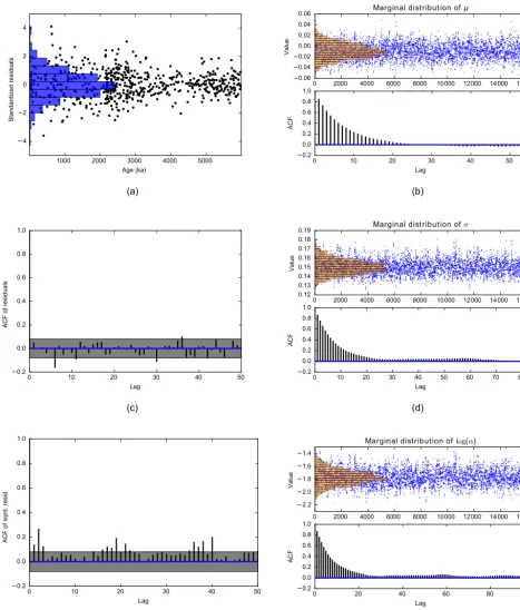
The decision of accepting or rejecting the null hypothesis is based on the periodogram evaluated atω, whose general formula is given in Eq. (64). The test is performed inde-pendently for each frequency (pointwise testing). Concretely, for each frequency, we compute the distribution of the peri-odogram under the null hypothesis, and then see if thedata periodogram at that frequency is above or below a given per-centile (e.g. the 95th) of that distribution. The perper-centile is calledlevel of confidence. If the data periodogram is above theXth percentile of the reference distribution, we reject the null hypothesis withX% of confidence. Thelevel of signif-icanceis equal to(100−X)%, e.g. a 95 % confidence level is equivalent to a 5 % significance level. Hypothesis test-ing is, for this reason, often called significance testing. See Fig. 8c and 8d for an illustration on paleoclimate data. We recommend Priestley (1981, chap. 6) for more details on the methodology.
To perform significance testing, we thus need
1. to estimate the parameters of the process under the null hypothesis (this is studied in Sect. 5.2);
2. to estimate the distribution of the periodogram under the null hypothesis (this is studied in Sect. 5.3).
5.2 Estimation of the parameters under the null hypothesis
5.2.1 Introduction
Under the null hypothesis, the signal is |Xi = |Trendi + |Noisei, and we thus need to estimate the parameters of the trend and those of the zero-mean CARMA process. The best statistical approach is to estimate them jointly, and marginalise over the parameters of the trend, since the pe-riodogram is invariant with respect to these parameters, ac-cording to Sect. 4.3. But this would imply very involved com-putations that are way beyond the scope of this work. We are thus forced to a compromise and proceed as follows: data are detrended,|Xdeti = |Xi −Psp{|t0i,|t1i,...,|tmi}|Xi, and then we
estimate the parameters of the CARMA process, based on the modelµ|t0i + |Noisei, where|Noiseiis a zero-mean sta-tionary Gaussian CARMA process sampled at the times of |ti.
Estimation of CARMA parameters is done in a Bayesian framework. We analyse separately the case of the white noise, which is done analytically, and the case of CARMA(p, q) processes with p≥1, for which Markov chain Monte Carlo (MCMC) methods are required. Bayesian analysis provides a posterior distribution of the parameters based on priors.
5.2.2 Gaussian white noise
We want to estimate the two parameters of the white noise, the meanµand the varianceσ2. According to the Bayes the-orem,
5(µ, σ2|D)=5 D|µ, σ 2
5 µ, σ2 5(D)
∼5D|µ, σ25µ, σ2, (78) where5is the probability density function (PDF) andDis the detrended dataXdet,1, . . ., Xdet,N. Based on the PDF of a
multivariate white noise, the likelihood function is
5(D|µ, σ2)
=
r
1 2π σ2
!N
exp −
PN
i=1 Xdet,i−µ2
2σ2
!
. (79)
We takeJeffreys priors(Jeffreys, 1946) forµandσ2:
5(µ, σ2)=5(µ)5(σ2),
with5(µ)∼1 and5(σ2)∼ 1
σ2. (80)
Since we do not actually need to estimateµ(see Sect. 4.3 and Formula 64), we marginalise over that variable,
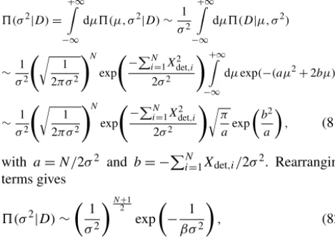
5(σ2|D)=
+∞ Z
−∞
dµ5(µ, σ2|D)∼ 1 σ2
+∞ Z
−∞
dµ5(D|µ, σ2)
∼ 1 σ2
r
1
2π σ2
!N
exp −
PN i=1X2det,i
2σ2
!+∞ Z
−∞
dµexp(−(aµ2+2bµ))
∼ 1 σ2
r
1 2π σ2
!N
exp
−PN
i=1X2det,i
2σ2
!r
π aexp
b2
a
, (81) with a=N/2σ2 and b= −PN
i=1Xdet,i/2σ2. Rearranging
terms gives
5(σ2|D)∼
1
σ2
N+21
exp
− 1
βσ2
, (82)
withβ=2/Nσˆ2, whereσˆ2=is the (biased) variance of the detrended data5. With the variable changey=1/σ2, we have
5(y|D)∼yN2−3exp(−y/β), (83)
which is nothing but a gamma distribution: 1
σ2
d
=γ
N−1
2 , 2
Nσˆ2
. (84)
Note that the mean of the distribution in Eq. (84) is equal to(N−1)/(Nσˆ2), which is the usual unbiased estimator of 1/σ2. Finally, the PDF ofσ2is at its maximum at
σmax2 = N
N+1σˆ
2. (85)
This is obtained from the derivative of Eq. (82). 5.2.3 Gaussian CARMA(p, q)noise withp≥1
For other cases than the white noise, Kelly et al. (2014) pro-vide robust algorithms to estimate the posterior distribution of the CARMA parameters and of the parameterµof an ir-regularly sampled, purely stochastic, time series, which can be modelled as a CARMA process. Those algorithms are based on Bayesian inference and MCMC methods. In par-ticular we recommend reading Sects. 3.3 and 3.6 of Kelly et al. (2014) for a discussion on the choice of the priors and for computational considerations, respectively. That paper is accompanied by a Python and C++ package calledCARMA pack. Some outputs of CARMA pack are shown in Sect. 9. 5.3 Estimation of the distribution of the periodogram
under the null hypothesis
5.3.1 Working with a trendless stochastic process Under the null hypothesis, the signal is |Xi = |Trendi + |Noisei =Pm
k=0γk|tki + |Noisei. The WOSA periodogram,
5σˆ2= 1
N
PN
i=1X2det,i−
1
N
PN
i=1Xdet,i 2
Eq. (64), is invariant with respect to the parameters of the trend, so that we can poseγk=0 for allkand|Xireduces to
a zero-mean CARMA process. 5.3.2 Monte Carlo approach
For each frequency, we need the distribution of the WOSA periodogram, Eq. (68), where|Xiis now a CARMA process for which we know the distribution of its parameters, from Sect. 5.2. With Monte Carlo methods, we are thus able to es-timate any percentile of the distribution of the periodogram. If|Xiis a zero-mean white noise,|Xiis sampled from a stan-dard normal distribution multiplied by the square root of the variance, whose inverse is sampled from the gamma distribu-tion (Eq. 84). If|Xiis a CARMA(p, q)process withp≥1, |Xiis generated with the Kalman filter (from the CARMA pack – see Sect. 5.2.3). An example of confidence levels is shown in Fig. 8d.
We are thus able to estimate confidence levels for the WOSA periodogram, taking into account the uncertainty in the parameters of the background noise.
5.3.3 Analytical approach
If we consider constant CARMA parameters, we show in this section that analytical confidence levels can be computed, even in the very tail of the distribution of the periodogram of the background noise. An example is given in Fig. 8c. The advantage of the analytical approach is twofold.
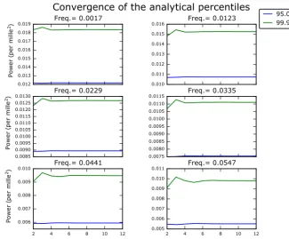
1. It provides confidence levels converging to the exact so-lution, as the number of conserved moments increases (see below). From a certain number of conserved mo-ments, we can consider that convergence is numerically reached (see Fig. 9). Such an approach is particularly interesting for high confidence levels, as illustrated in Fig. 8c with the 99.9 % confidence level, for which a MCMC approach would require a huge number of sam-ples to get a satisfactory accuracy.
2. As a consequence, for a given percentile, computing time is usually shorter with the analytical method than with the MCMC method. We note, however, that the MCMC approach generally needs less computing time when the number of data points becomes large, as shown in Appendix E.
First approximation
If the marginal posterior distribution of each CARMA pa-rameter is unimodal, we take the papa-rameter value at the max-imum of its PDF (white noise case, see Eq. 85), or the me-dian parameter6(other cases). Note that multi-modality tends
6For CARMA processes with p >0 andq≥0, the marginal
to appear more frequently for CARMA processes of high or-der. Working with a unique set of parameters allows us to find an analytical formula for the distribution of the WOSA periodogram. Considering the matrix forms of the CARMA noise (Eq. 20 or 38) and the WOSA periodogram (Eq. 68), we demonstrate the following theorem.
Theorem 1. The WOSA periodogram, defined in Eq. (68), under the null hypothesis (76), is
||PWOSA(ω)|Xi||2 d
= 2Q(ω)
X
k=1
λk(ω)χ12k, (86)
where |Xi =Pm
k=0γk|tki +K|Zi,Kis the CARMA matrix
defined in Eq. (20) or (38), andQ(ω)is the number of WOSA segments atω.
χ12
1, ...,χ
2
12Q(ω) are iid chi-square distributions with1
de-gree of freedom, andλ1(ω), ...,λ2Q(ω)(ω)are the eigenvalues
ofM0
ωKK
0M
ω and are non-negative. MatrixMω is defined
in Eq. (69).
Proof.Since the WOSA periodogram, Eq. (68), is invariant with respect to the parameters of the trend, we pose them as equal to zero and consider the zero-mean CARMA process
|Xi =K|Zi. (87)
The periodogram is thus
||PWOSA(ω)|Xi||2= hZ|K0MωM0ωK|Zi = hγ|γi, (88)
with |γi =M0ωK|Zi. Since |Zi is a standard multivariate normal distribution, we have
|γi=d N(0,M0ωKK0Mω). (89)
M0ωKK0Mω is a (2Q(ω),2Q(ω)) real symmetric positive
semi-definite matrix. We can thus diagonalise it:
∃an orthogonal matrixUs.t.U0M0ωKK0MωU=D, (90)
withDbeing a diagonal matrix with the 2Q(ω)non-negative eigenvalues ofM0ωKK0Mω. We now haveU0|γi
d
=N(0,D), and
||PWOSA(ω)|Xi||2= hγ|γi = hγ|UU0|γi = hZ|
√ D
√ D|Zi=d
2Q(ω)
X
k=1
λk(ω)χ12k, (91)
where theχ12
k distributions are iid.
The pseudo-spectrumis defined as the expected value of the periodogram distribution:
b S(ω)=
2Q(ω)
X
k=1
λk(ω)=tr M0ωKK
0
Mω
. (92)
such as smoothing the distribution. A simple alternative is to take the median.
The difference between the pseudo-spectrum and the tradi-tionalspectrumis explained in Appendix C.
If the background noise is white, we have K=σI and this implies that tr(M0ωKK0Mω)=tr(M0ωMω)σ2=
tr(MωM0ω)σ2=2σ2, such that the pseudo-spectrum is
bS(ω)=2σ2, (93)
and is thus flat. This is a well-known result of the LS peri-odogram (Scargle, 1982), generalised here to more evolved periodograms. Moreover, if there is no WOSA segmentation (Q(ω)=1∀ω), the periodogram is exactly chi-square dis-tributed with 2 degrees of freedom:
||Psp{|t0i,|t1i,...,|tmi,|Gcωi,|Gsωi}−Psp{|t0i,|t1i,...,|tmi}
σ|Zi||2
d
=σ2χ12
1+σ
2χ2 12
d
=σ2χ22, (94)
which is also a generalisation of a well-known result of the LS periodogram (Scargle, 1982).
The variance of the distribution of the periodogram, Eq. (86), is equal to 2P2Q(ω)
k=1 λ 2
k(ω)=2||M
0
ωKK
0M
ω||2F, where|| · ||Fis the Frobenius norm. As expected, it decreases withQ, as illustrated in Fig. 3.
Going back to Eq. (86), it is well-known that a linear com-bination of (independent)χ2distributions is not analytically solvable. Fortunately, excellent approximations are available in Provost et al. (2009), allowing Monte Carlo methods to be avoided.
Second approximation
We approximate the linear combination of independent chi-square distributions, conserving its firstd moments. When
d→ ∞, the approximation converges to the exact distribu-tion. In practice, estimation of a percentile is already very good with a very few moments, as illustrated in Fig. 9. Let us proceed step by step by increasing the number of conserved moments. DefineX=P2Q(ω)
k=1 λk(ω)χ12k.
1-moment approximation
We require the expected value of the process to be conserved, which is satisfied with the following approximation:
X≈d 1 2Q(ω)
"2Q(ω) X
k=1
λk(ω)
#
χ22Q(ω), (95)
or, equivalently,
X≈d 1
2Q(ω)bS(ω)χ
2
2Q(ω). (96)
2-moment approximation
0.000 0.005 0.010 0.015 0.020 0.025 0.030 Frequency (ka− 1)
102 103 104 105 106 Variance
Analytical variance of the WOSA periodogram for the background noise
Q = 1 Q = 8 Q = 19 Q = 36
Figure 3. Analytical variance of the WOSA periodogram for a Gaussian red noise withσ=2 andα=1/20 (see Sect. 3.2.3 for the definition of a red noise) for different values ofQ. The frequency range is chosen such that, for each curve,Q(ω)is constant all along. The red noise is built on the irregularly sampled times of ODP1148 core (see Sect. 9).
conserve the expected value and variance. A chi-square dis-tribution withMdegrees of freedom provides a good fit:
X≈d gχM2. (97)
Equating the expected values and variances gives
M=(tr(A)) 2 ||A||2
F
andg=||A|| 2 F
tr(A), (98)
whereA=M0ωKK0Mω and||A||2Fis the squared Frobenius norm of matrix A, i.e. the sum of its squared eigenvalues. Note thatgχM2 =d γM/2,2g, where 2g is thescaleparameter
of the gamma distribution, which motivates the followingd -moment approximation.
Thed-moment approximation
We apply here the formulas presented in Provost et al. (2009). LetfXbe the PDF ofX. This distribution is approximated by
the PDF of adth degree gamma-polynomial distribution:
fX(x)≈γα,β(x) d
X
i=0
ξixi, x≥0, (99)
where the parameters α and β are estimated with the 2-moment approximation detailed above, andξ0, ...,ξdare the
solution of ξ0 ξ1 . . . ξd =
η(0) η(1) . . . η(d−1) η(d) η(1) η(2) . . . η(d) η(d+1)
. . . . . . . . . . . . . . . η(d) η(d+1) . . . η(2d−1) η(2d)
−1
1 µ(1)
. . . µ(d) . (100)
Here, µ(1), ..., µ(d) are the exact first d moments of X
and can be computed analytically by recurrence (see Eq. 5 of Provost et al., 2009), andη(h)is thehth moment of the gamma distribution,η(h)=βh0(α+h)/ 0(α). The approx-imate cumulative distribution function (CDF) ofX, evaluated atc0, is then
FX(c0)≈ 1
0(α)
d
X
i=0
ξiβiγ (i+α, c0/β) , c0>0, (101)
whereγ (s, x)is the lower incomplete gamma function:
γ (s, x)=
x
Z
0
dt ts−1exp(−t ). (102)
After all that chain of calculus, we reached our objective, that is, the estimation of a confidence level for the WOSA periodogram. It is given by the solutionc0of
1
0(α)
d
X
i=0
ξiβiγ (i+α, c0/β)−p=0, (103)
for some p value p, e.g. p=0.95 for a 95 % confidence level.
The gamma-polynomial approximation can be extended to the generalised gamma-polynomial approximation. The latter is based on the generalised gamma distribution and is defined in Appendix D. It gives percentiles that usually converge faster than those given by the gamma-polynomial approximation. However, we observed that the generalised gamma-polynomial approximation is quite sensitive to the quality of the first guess for the three parameters of the gen-eralised gamma distribution (see Appendix D). We thus rec-ommend the use of the gamma-polynomial approximation as a first choice. Both options are available in WAVEPAL.
Finally, we mention that there exists an alternative expres-sion to the above development, in terms of Laguerre poly-nomials (see Provost, 2005). It has the advantage of not re-quiring the matrix inversion in Eq. (100), the latter possibly being singular at large values of the degreed. However, we have not found any improvement on the stability or comput-ing time uscomput-ing that approach.
5.4 The F periodogram for the white noise background We have shown in Eq. (94) that the periodogram of a Gaus-sian white noise is exactly chi-square distributed if there is no WOSA segmentation. Significance testing against a white noise requires the estimation of the white noise variance af-ter having detrended the data. Knowing that a F distribution is the ratio of independent chi-square distributions, it is pos-sible to get rid of the detrending and variance estimation and deal with a well-known distribution, by working with
(N−m−3)||P
sp{|t0i,|t1i,...,|t mi,|cωi,|sωi}−Psp{|t0i,|t1i,...,|t mi}
|Xi||2
2||I−P
sp{|t0i,|t1i,...,|t mi,|cωi,|sωi}
We call it theF periodogram. We already know that the nu-merator is invariant with respect to the parameters of the trend of the signal. It is clear that the denominator is invariant with respect to the parameters of the trend as well as with re-spect to the amplitudes of the periodic components (only the |Noiseiterm remains when applying it to Eq. 13). Moreover, that ratio is invariant with respect to the variance of the sig-nal. Last but not least, the orthogonal projections in the nu-merator,[Psp{|t0i,|t1i,...,|tmi,|cωi,|sωi}−Psp{|t0i,|t1i,...,|tmi}], and
in the denominator,[I−Psp{|t0i,|t1i,...,|tmi,|cωi,|sωi}], are done
on spaces that are orthogonal to each other. Consequently, if we consider the null hypothesis (76) with a white noise, the numerator and the denominator followindependent chi-square distributions, and
(N−m−3)||(Psp{|t0i,|t1i,...,|tmi,|cωi,|sωi}−Psp{|t0i,|t1i,...,|tmi})|Xi|| 2
2||(I−Psp{|t0i,|t1i,...,|tmi,|c
ωi,|sωi})|Xi|| 2
d
=(N−m−3)χ 2 2 2χN2−m−3
d
=F (2, N−m−3), (105)
where |Xi=d
m
X
k=0
γk|tki +N
µ, σ2
d
= |Trendi +Nµ, σ2, (106)
and whereF (2, N−m−3)is the Fisher–Snedecor distribu-tion with parameters 2 andN−m−3. In conclusion, the F pe-riodogram can be an alternative to the pepe-riodogram when performing significance testing. It has the advantage of not requiring any parameter to be estimated and applies under the following conditions.
– The background noise is assumed to be white. – There is no WOSA segmentation.
– There is no tapering.
The F periodogram is available in WAVEPAL under the above requirements.
With a WOSA segmentation, projections at the numera-tor and at the denominanumera-tor are not performed any more on orthogonal spaces, and this cannot therefore be applied.
The above results are a generalisation of formulas in Brockwell and Davis (1991) and Heck et al. (1985). See Ap-pendix F for additional details.
6 The amplitude periodogram 6.1 Definition
Going back to Eq. (13), we now look for the amplitude
Eω=
p A2
ω+Bω2at a given frequencyf =2ωπ. The
estima-tion ofEω2 is called theamplitude periodogram and is de-noted byEbω2. We estimate Aω andBω with a least-squares
approach. We start with a trendless signal, and will show that the amplitude periodogram and the periodogram are approx-imately proportional.
6.2 Trendless signal 6.2.1 No tapering
The estimated amplitudes we look for,Abω andBbω, are the
solution of
b
Aω,Bbω= argmin
{(A,B)∈R2}
|| |Xi −(A|cωi +B|sωi)||2. (107)
Since we look for the minimal distance, the solution is given by the orthogonal projection onto the vector space spanned by|cωiand|sωi, namely
Psp{|cωi,|sωi}|Xi =Abω|cωi +Bbω|sωi. (108)
Let us develop this equation: Vω2(V
0
ω2Vω2) −1V0
ω2|Xi =Vω2|8bωi, (109)
where
Vω2=
| |
|cωi |sωi
| |
and|8bωi =
b Aω
b Bω
, (110)
and we find the well-known expression for the solution of a least-squares problem:
|b8ωi = V0ω2Vω2
−1
V0ω
2|Xi. (111)
Finally,
b
Eω= |||b8ωi||. (112)
In the regularly sampled case, at the Fourier frequencies, the amplitude periodogram is proportional to the periodogram, with a factor 2/N (or a factor 1/N atω=0 andω=π/1t; the projection being done on the single cosine at those fre-quencies). It is no longer the case with irregularly sampled time series, and the proportionality is only approximate:
b Eω2≈ 2
N||Psp{|cωi,|sωi}|Xi||
2. (113)
To prove the above formula, rewrite the model (Eq. 13) at
=ω:
|Xi =Eωcos(ω|ti +φω−βω+βω)+ |Noisei (114)
=Aωcos(ω|ti −βω)+Bωsin(ω|ti −βω)+ |Noisei,
whereβωis defined in Eq. (42) and makes the phase-lagged
same expressions as in Eq. (13), but we still haveEω2=A2ω+
Bω2. We can rewrite Eq. (111) but this time withVω2holding
the above phase-lagged sine and cosine. We now make use of the approximation stated in Lomb (1976, p. 449):
N
X
i=1
cos2(ωti−βω)≈
N
2 and
N
X
i=1
sin2(ωti−βω)≈
N
2. (115)
Note that the sum of both is exactly equal to N. Equa-tion (113) is then obtained, observing that V0ω
2Vω2≈ N
2I. Basic trigonometry gives the following equalities for the rel-ative error of the above approximations:
PN
i=1cos2(ωti−βω)−N/2
N/2
=
PN
i=1sin2(ωti−βω)−N/2
N/2
=
PN
i=1cos(2(ωti−βω))
N
, (116)
so that the two approximations of Eq. (115) reduce to only one:
PN
i=1cos(2(ωti−βω))
N ≈0. (117)
The quality of this approximation is illustrated in Fig. 4. 6.2.2 With tapering
Like with the periodogram, leakage also appears in the am-plitude periodogram. Consequently, it may be better to work with the projection on tapered cosine and sine if the data are not too irregularly sampled, as explained in Sect. 4.4. Con-sideration of the tapered case is also an important mathemat-ical prerequisite for an extension to the continuous wavelet transform. This is developed in Part 2 of this study (Lenoir and Crucifix, 2018).
b
Aω andBbωare determined by projecting the data onto
ta-pered cosine and sine:
Psp{|Gcωi,|Gsωi}|Xi =Abω|cωi +Bbω|sωi. (118)
Developing the equation gives |b8ωi = V0ω2GVω2
−1
V0ω
2G|Xi, (119)
and
b
Eω= |||b8ωi||, (120)
where Vω2 is defined in Sect. 6.2.1 and G is defined in
Sect. 4.4.
0.0 0.1 0.2 0.3 0.4 0.5
0 5 10 15 20
Abs. error (%)
(a)
0.0 0.1 0.2 0.3 0.4 0.5
0 5 10 15 20
Abs. error (%)
(b)
0.0 0.1 0.2 0.3 0.4 0.5
Freq. (ka )− 1
0 5 10 15 20
Abs. error (%)
(c)
Figure 4. Illustration of the quality of the approximations
(a)Eq. (123a),(b)Eq. (123b) and(c) Eq. (126). In blue: no ta-pering (square taper); in green: sin2taper; in red: Gaussian taper. The approximation (117) is thus in blue in panel(a)or(b). Each panel represents the left-hand side of the equation, multiplied by 100, to express percentage. This indicates how small the numerator is compared to the denominator. The time vector|ticomes from the
ODP1148 core (see Sect. 9) for which1tGCD=1 kyr.
Note that the approach we follow does not correspond to the classical least-squares problem as above since, in Eq. (118), the cosine and sine are tapered only on the left-hand side of the equality. However, one can reconstruct a sig-nal from its projection coefficients with a different function than the one which is used to determine those coefficients (see Torrésani, 1995, Eq. II.8, p. 15, in which the similarity toVω2|8bωi =Vω2(V
0
ω2GVω2) −1V0
ω2G|Xiis evident). Note
thatVω2(V 0
ω2GVω2) −1V0
ω2Gis a projection, since it is
idem-potent, but the projection is not orthogonal, because it is not symmetric.
Similarly to the non-tapered case, we now determine an approximate proportionality between the amplitude pe-riodogram and the tapered pepe-riodogram. We start with the model (Eq. 13) evaluated at=ωand written under the fol-lowing form
|Xi =Aωcos(ω|ti −βω)+Bωsin(ω|ti −βω)
+ |Noisei, (121)
whereβω is introduced such thathGcω|Gsωi =0, or
equiva-lently, such thatV0
ω2G
2V
ω2 is diagonal. A little development
gives the formula for determiningβω:
tan(2βω)=
PN
i=1G2iisin(2ωti)
PN
i=1G2iicos(2ωti)