Likelihood Based Confidence Sets for the Timing of Structural Breaks

Munich Personal RePEc Archive

Likelihood-Based Confidence Sets for the

Timing of Structural Breaks

Eo, Yunjong and Morley, James C.

Washington University in St. Louis, Washington University in St.

Louis

5 September 2008

Online at

https://mpra.ub.uni-muenchen.de/13913/

Likelihood-Based Confidence Sets for the

Timing of Structural Breaks

∗

Yunjong Eo and James C. Morley

Department of Economics

Washington University in St. Louis

Campus Box 1208, One Brookings Drive

St. Louis, MO 63130-4899

Job Market Paper

This draft: October 25 2008

Abstract

In this paper, we propose a new approach to constructing confidence sets for the timing of structural breaks. This approach involves using Markov-chain Monte Carlo methods to simulate marginal “fiducial” distributions of break dates from the like-lihood function. We compare our proposed approach to asymptotic and bootstrap confidence sets and find that it has the best overall finite-sample performance in terms of producing short confidence sets with accurate coverage rates. Our approach has the advantages of i) being broadly applicable to different patterns of structural breaks, ii) being computationally efficient, and iii) requiring only the ability to evaluate the like-lihood function over parameter values, thus allowing for many possible distributional assumptions for the data. In our application, we investigate the nature and timing of structural breaks in postwar U.S. Real GDP. Based on marginal fiducial distribu-tions, we find much tighter 95% confidence sets for the timing of the so-called “Great Moderation” than has been reported in previous studies.

Keywords: Fiducial Inference; Bootstrap Methods; Structural Breaks; Confidence Intervals and Sets; Coverage Accuracy and Expected Length; Markov-chain Monte Carlo;

JEL classification: C15(Simulation Methods); C22 (Time-Series Models)

∗_{We thank Jeremy Piger, Werner Ploberger, Junsoo Lee, Tao Zha, members of the applied time series}

research group at Washington University,and participants at the 2008 North American Summer Meeting of the Econometric Society, the 2008 Missouri Economics Conference, the 2008 NBER-NSF Time Series Conference, and 2008 Midwest Econometrics Group for helpful comments. All errors are our own.

1

Introduction

In this paper, we propose a new approach to constructing confidence sets for the timing

of structural breaks in time series.1 Our proposed approach involves simulating marginal

“fiducial” distributions of break dates from the likelihood function. The practical

imple-mentation of this approach utilizes Markov-chain Monte Carlo (MCMC) methods that have

been widely used for posterior simulation in the Bayesian literature. Indeed, the resulting

confidence sets are the same as Bayesian highest-posterior-density (HPD) credible sets given

noninformative priors. However, we take a strictly classical viewpoint with respect to our

inferences about the confidence sets by considering their coverage accuracy and expected

length across repeated samples.

In order to motivate our use of “fiducial” distributions to construct confidence sets, it

is necessary to discuss fiducial inference, which was first developed by Fisher (1930) and

involves making probability statements about parameters, with the probabilities being

pro-portional to the likelihood function and having a frequentist interpretation.2 _{While the idea}

of making probability statements directly about parameters is antithetical to the standard

classical viewpoint, it has long been understood that there can be, in certain settings, a close

relationship between fiducial confidence sets and classical confidence sets. In particular, in

the case of a single parameter for which a pivotal test statistic is available, fiducial confidence

sets and the classical confidence sets based on inverting the test statistic will be the same,

even if their interpretation is different.3 _{Thus, our strategy here is to use fiducial}

distribu-tions as a means of generating a classical estimator for a confidence set, much in the same

way as a likelihood function is used to generate a classical estimator for a model parameter.

1

Because our approach can produce disconnected subsets of possible break dates, we prefer the termi-nology of “confidence set” to “confidence interval”, although we still refer to “length” rather than “size” of a confidence set to make it clear that we are considering inferences about a single parameter, rather than a multi-dimensional confidence region.

2

For more details about fiducial inference, see Fraser (1961a,b). Barnett (1999) provides an accessible and in-depth discussion of the issues surrounding fiducial inference in his textbook on comparative methods of statistical inference. Recently, Hannig (2006) argues for the fiducial approach as a tool for deriving classical inference procedures, which is the general strategy that we take in this paper.

3

Our proposed approach can be related to some existing methods for constructing

con-fidence sets. It is most directly analogous to Sims and Zha (1999), who consider Bayesian

credibility sets based on noninformative priors as a means of constructing classical “error

bands” for impulse response functions in structural Vector Autoregressive (VAR) models.

On a more general level, our approach has a similar motivation to bootstrap methods for

constructing confidence sets (see, for example, Kilian (1999) and MacKinnon (2002)).

Specifically, while bootstrap confidence sets will only be exact when based on a pivotal

quantity, they appear to perform well, and notably better than confidence bands based

on asymptotic distributions, in settings when a bootstrap distribution approximates

finite-sample distributions that are close to being pivotal. Along these lines, we consider the

possibility that a marginal fiducial distribution implicitly provides an even better

approx-imation of finite-sample distributions that are even closer to being pivotal. Meanwhile,

because our approach uses marginal distributions, it can also be related to the extensive

testing literature in which nuisance parameters are integrated out of the likelihood (see, for

example, Andrews and Ploberger (1994)).4 _{Indeed, our approach is directly motivated by}

Elliott and M¨uller (2007), who propose constructing confidence sets for the timing of

struc-tural breaks by inverting a test statistic for which nuisance parameters have been integrated

out.

In the specific setting of making inferences about the timing of structural breaks, we

compare our fiducial distribution (FD) approach to a range of asymptotic and bootstrap

methods. In terms of asymptotic methods, Bai (1997) provides the standard approach

to constructing a confidence interval for a single break, Bai, Lumsdaine, and Stock (1998)

consider multivariate models, and Bai and Perron (2003) allow for multiple structural breaks.

Elliott and M¨uller (2007) show that Bai’s approach attains very low coverage rates when

structural breaks in parameters are small and they propose an approach, mentioned above,

that is based on inverting sequential tests over the parameter space of break dates. Their

approach attains more accurate coverage rates than Bai’s approach, but at the cost of much

4

longer confidence sets. Meanwhile, in terms of bootstrap methods, we are motivated, in

part, by Diebold and Chen (1996)’s comparison of asymptotic and bootstrap methods for

testing the existence of structure change. They find that, especially for smaller samples and

persistent dynamics, the bootstrap approximation to the finite-sample distributions of these

tests is usually more accurate than the asymptotic approximation. Here, we use bootstrap

methods to construct confidence sets for the break dates themselves. In terms of bootstrap

methods, we consider constructing confidence sets using a “bootstrap percentile” approach, a

“bootstrap standard error” approach, a “bootstrap inverted likelihood ratio (LR)” approach,

and an approach based on a bootstrap of Bai’s (1997) asymptotically pivotal statistic.

In order to compare the finite-sample performance of various methods of constructing

confidence sets for break dates, we conduct Monte Carlo analysis of coverage accuracy and

expected length. This analysis suggests that in small samples with structural breaks of

the kind hypothesized for economic time series such U.S. real GDP, the FD and bootstrap

inverted LR approaches produce relatively short confidence sets while maintaining accurate

coverage rates compared to nominal confidence levels. Indeed, for sample sizes of 320 and

640, which can be compared with 238 observations for postwar quarterly real GDP between

1947:Q1 and 2005:Q2, the confidence sets for these two likelihood-based approaches are

approximately from about a half to one fourth as long as those of other methods, while

always attaining exact coverage rates.5 _{For example, while Elliott and M¨uller’s inverted test}

approach succeeds in having accurate coverage rates, the average length of confidence sets for

the timing of a break in long-run growth is 40 periods for a sample size of 320 versus only 15

periods using the FD approach. Meanwhile, as discussed in Elliott and M¨uller (2007), Bai’s

confidence sets attain too low coverage rates compared to the nominal confidence levels.

The Monte Carlo analysis supports the use of likelihood-based confidence sets for the

timing of structural change. Beyond this analysis, however, there are additional practical

5

reasons to use likelihood-based confidence sets and the FD approach in particular.

First, the FD approach is broadly applicable in the sense that we can easily consider

structural breaks in different parameters occurring at different dates. This more complicated

pattern of structural breaks has been hypothesized for U.S. real GDP and other

macroeco-nomic time series. In particular, Kim and Nelson (1999) and McConnell and Perez-Quiros

(2000) detect the break date of the volatility deduction in 1984:Q1, while Zivot and Andrews

(1992) and others find that there is a trend break in 1972:Q2 in the unit root literature.

Stock and Watson (1996, 2002) show that most of U.S. macroeconomic data are unstable

and have volatility changes. Among the methods considered here, only the FD and bootstrap

approaches can construct confidence sets for different break dates of different parameters,

such as a mean and a variance changing at different points of the sample. However, in this

setting, the bootstrap approaches produce multi-dimensional confidence regions, rather than

confidence sets for each of the individual structural breaks. To get a confidence set for a

specific break date, we would need to integrate out other break dates, but the integration

is generally infeasible for a bootstrap.6 _{By contrast, integrating out break dates and other}

parameters is a straightforward feature of the FD approach.

Second, although bootstrap methods are available for general settings, the FD approach

is much more computationally efficient, especially for more complicated structural changes

(e.g., respective breaks in mean and variance). Suppose, for example, we have 100

obser-vations for an econometric model with two parameters such as a constant and a variance

and both parameters have structural breaks, but at different dates. Implementing bootstrap

methods for this model is computationally costly because for each bootstrap data set we

would need to consider 10,000 (=100×100) combinations of two break dates and estimate

break dates as well as model parameters, a mean and a variance before and after breaks,

6

simultaneously by maximum likelihood estimation (MLE).7 _{In the case of 199 bootstraps,}

which is a relatively small number of artificial samples, we would need to conduct MLE

1,990,000 (=199×10,000) times. To give a sense of this number, even if it takes just one

second per estimation, 1,990,000 cases would take more than 23 days.

Third, the FD approach requires only the ability to evaluate the likelihood function over

parameter values and potential break dates. Thus, it can be applied given any econometric

model with a specified likelihood function (e.g., models with normal distributions, Student-t

distributions, Poisson distributions, and so on). While the bootstrap inverted LR approach

is also available, in principle, for any specified likelihood function, computational difficulties

become an issue again. This is because numerical optimization over the entire parameter

space can be challenging for non-normal models due to irregularities in the likelihood surface.

By contrast, the evaluation of the likelihood for the FD approach via MCMC methods can be

broken down into more manageable steps. In addition, we only need to evaluate the likelihood

for the actual data, as opposed to considering restricted and unrestricted likelihoods for the

actual data and for each bootstrap sample in the case of the bootstrap inverted LR approach.

For our application, we examine the nature and timing of structural breaks in postwar

U.S. real GDP. First, we apply sequential tests to determine the number and types of

struc-tural breaks. Then, for each break, we employ the various methods of constructing confidence

sets considered in our Monte Carlo analysis to make inferences about their timing. Under

the assumption of a unit root, we find support for the Great Moderation in the form of a

variance reduction in quarterly growth rates, with the maximum likelihood estimate of the

break in 1984:Q1 and a narrow 95% confidence set of 1982:Q1 to 1984:Q4 based on the FD

approach. Notably, this 95% confidence set is smaller than the 67% confidence set based on

Bai’s (1997) approach reported in Stock and Watson (2002). In our application, the lengths

of the confidence sets based on Bai’s method are more than twice as long as those based on

FD approach. Meanwhile, given a unit root, we find no significant evidence of a break in

the long-run growth rate, so we do not construct a confidence set for such a break in this

case. On the other hand, under the assumption of trend stationarity, we do find significant

7

evidence of a structural break in the form of a reduction in drift, with the maximum

likeli-hood estimate of the break in 1969:Q1. However, the confidence sets for the timing of the

drift break are far from precise. For example, the outer bounds of the FD confidence set

are 1963:Q2 and 1983:Q3, respectively.8 _{Again, we find evidence for the Great Moderation}

under the assumption of trend stationarity, with maximum likelihood estimate of the break

in 1982:Q4 and a narrow FD confidence set from 1982:Q3 to 1984:Q2. Finally, we check the

robustness of our inferences for the FD approach by allowing for Student-t distributed errors

in our structural break models and we find that the resulting confidence sets for the Great

Moderation are very similar to the normal error case.

The remainder of this paper is organized as follows. Section 2 provides details for the

various methods of constructing confidence sets for structural break dates. Section 3

dis-cusses asymptotic theory related to these methods. Section 4 reports Monte Carlo results

for coverage accuracy and length of the confidence sets for the various methods under

con-sideration. Section 5 presents estimation results for models that capture structural breaks in

postwar U.S. real GDP and reports confidence sets for the timing of the structural breaks.

Section 6 concludes.

2

Methods

In this section, we provide details of our proposed FD approach to constructing confidence

sets for the timing of structural breaks. We also review the asymptotic methods presented

in Bai (1997) and Elliott and M¨uller (2007) and introduce various bootstrapping methods:

a bootstrap percentile approach, a bootstrap standard error approach, a bootstrap inverted

LR approach, and a bootstrap of Bai’s statistic. Previous Monte Carlo studies of bootstrap

methods in other settings have shown that no specific approach is always superior in terms

of coverage accuracy. For example, see MacKinnon (2002) for confidence intervals of regular

parameters and Kilian (1999) for confidence intervals of impulse responses for VAR models.

Thus, we consider various methods here in order to determine which ones work best in the

8

context of structural breaks.

In terms of possible patterns of structural breaks, we consider a linear econometric model

that allows the variance and coefficients to undergo breaks at different dates.

yt=

K X

k=1

X_kt′ βkt+Z_t′γ+et, et_∼i.i.d._N(0, σ2_t), t= 1, ..., T (1)

where

σ_t2 =



      

      

σ2

0 if 1≤t ≤τK+1,1 σ12 if n1 < t≤τK+1,2

...

σ2

N if nN < t≤T .

The model in (1) has K subsets of regressors, Xkt’s, k = 1, ..., K. Each subset has qk

regressors, corresponding to kth group of regressors. That is, each subset of regressors

has its own change-point system. In particular, each subset may have a different number of

breaks occurring at different dates than those of other groups independently.9 _{The coefficient}

vector βkt is βkj (kth group’s j + 1th regime parameters) if τkj < t ≤ τkj+1, j = 0, .., Mk.

The number of breaks for kth subset is denoted by Mk. Zt and γ represent regressors and

their respective coefficients that do not change. The variance can have N breaks and nth

regime’s variance is σ2

n−1. In practice, the potential break dates are restricted between the

middle (1₋2λ) portion of the sample period, Π = [λT,(1₋λ)T], to avoid an end of sample

distortion. Two consecutive break dates are also at least a distance of λof the total sample

size apart for a similar reason.

2.1

Confidence Sets Based on Marginal Fiducial Distributions

In order to derive the marginal fiducial distributions for break dates, letf(y_|ψ, τ) denote the

probability density function (pdf) for a model with structural break date(s)τand parameters

ψ = (β, γ, σ)_∈ Ψ in (1) evaluated at the observed data Y =y. The likelihood function for

the model is defined by L(ψ, τ|y) = f(y|ψ, τ) since the break date τ can be interpreted as

9

a parameter. Then, briefly ignoring problems of interpretation, a joint pdf for ψ and τ can

always be constructed, at least in principle, by simply multiplying the likelihood function by

the inverse of its integral (or summation) with respect to model parameters:

π(ψ, τ_|y) =L(ψ, τ_|y)_×[

(1−λ)T X

τ=λT Z

Ψ

L(ψ, τ_|y)dψ]−1. (2)

Interpreting these probabilities as having meaning in a frequentist sense is called fiducial

inference and is highly controversial in the statistics literature (see Barnett (1999) for a

discussion of the controversies surrounding fiducial inference).

In this paper, we do not address the debate over the general coherence of fiducial inference.

Our goal here is merely to use fiducial distributions as a means of making more traditional

classical inferences. Importantly, we do not directly consider the joint fiducial distribution in

(2) because fiducial and classical confidence intervals are generally at odds with each other

in multidimensional cases. Instead, we consider the marginal fiducial distributions for the

break dates:

π(τ_|y) =

Z

Ψ

π(ψ, τ_|y)dψ (3)

In particular, for a single parameter and given a pivotal test statistic for that parameter,

fiducial and classical confidence sets based on inverting the statistic are the same. Thus,

if we assume that there exists a test statistic whose distribution is related to the marginal

fiducial distribution of a parameter and it is close to being pivotal, even in finite samples,

the fiducial confidence intervals will be the similar to classical confidence intervals based on

inverting that test statistic. The key point, then, in using fiducial distributions is that we

can construct the classical confidence interval without directly having the test statistic.

As mentioned in the introduction, we see our approach as similar to bootstrap analysis. If

the finite-sample distribution of the likelihood-based test statistic were pivotal, the confidence

set based on the marginal fiducial distributions would be exact. Meanwhile, even if the

finite-sample distributions are not strictly pivotal, the FD confidence sets could reflect a better

or bootstrap methods.

The most obvious potential problem with using marginal fiducial distributions to

con-struct confidence sets is finding these distributions in the first place. In particular, it is

generally infeasible to use analytical methods to integrate the likelihood function with

re-spect to model parameters in order to get the denominator in (2) and then to integrate the

resulting joint fiducial distribution to get the marginal fiducial distribution (3). However,

the marginal fiducial distributions of model parameters can be easily simulated via MCMC

methods.10 _{In particular, suppose the parameters and break date(s) in the model are grouped}

into two different blocks: ψandτ, respectively. The parameters in one block can be sampled

conditional on data and the parameters in the other block. For model parameters, ψ,

ψ _∼ π(ψ|τ,y)

∝ π(ψ)f(y_|ψ, τ)

∝ f(y_|ψ, τ).

For break dates,τ,

τ ∼π(τ|ψ,y)

where

π(τ_|ψ,y) = π(τ)f(y|ψ, τ)

π(y_|ψ)

= Pπ(τ)f(y|ψ, τ) τπ(τ)f(y|ψ, τ)

= Pf(y|ψ, τ) τf(y|ψ, τ)

.

The MCMC method simulates parameter values from their conditional distributions until

the draws behave as if drawn from their joint and marginal distributions. Because the

parameters of the denominator in (2) are uniformly integrated, π(ψ) and π(τ) should be

10

chosen to be constant over parameter values. For example, π(τ) of one break model is from

a uniform distribution on the integers:

π(τ) =





 1

(1−2λ)T f or τ ∈[λT,(1−λ)T]

0 otherwise.

Then, the draws behave exactly same as draws from the marginal fiducial distribution in

(3) based on integrating the other parameters and break dates out of the joint fiducial

distribution in (2). A more detailed MH algorithm used in this paper is presented in an

appendix.

Given a simulated marginal fiducial distribution for a break date, we can then construct

a confidence set at a 1₋ α level in different ways. In practice, we choose to construct

the confidence set using the Bayesian highest-posterior-density (HPD) concept in order to

obtain the shortest confidence sets possible for a given confidence level.11 In particular, the

confidence set is

S(y) ={τ|π(τ|y)≥k(1−α)} (4)

wherek(1−α) is the largest constant satisfying π(S|y)≥1−α. Since the break dates have discrete distributions, it is straightforward to find points with highest probability because

the simulated marginal fiducial distributions produce different simulated frequencies for each

possible break date.12 _{When we apply this highest probability concept to constructing the}

confidence set from the marginal fiducial distribution, the result is a “highest-fiducial density”

(HFD) confidence set.

Three issues should be addressed here.

11

The notion that lengths of confidence sets with the same confidence levels can differ and shorter ones are to be preferred can be illustrated by the following simple example: ConsiderT observations of a scalar random variable,_{x1, . . . , xT}, normally distributed with unknown meanµand known variance 1. We want

to construct a confidence interval of the true µ by using the observations. We can think of two different confidence interval estimators that have a 95% confidence level: [_−∞,¯x+ 1.65/√T] and [₋1.96/√T+ ¯x,¯x+ 1.96/√T] where ¯x is the sample mean. Both confidence intervals would include the true mean µ with probability 0.95 when computed over repeated samples. However, the length of the former is infinite, while that of the latter is only 3.92/√T. Thus, the former provides much more information about the true µ

than the latter in the sense that we can narrow the range of the true value. Thus, we would prefer shorter confidence interval, all else equal.

12

First, in a classical context, the confidence set at any given confidence level 1−α can

only be justified through its coverage rate in repeated samples. This means that if we could

compute confidence sets for infinitely many data sets from population, they would include the

true value of the parameter in 100_×(1₋α)% of the data sets. Letτ0 andC(Y) denote a true

break date and any usual classical confidence set estimator, with Y having the distribution

f(y_|τ0) that depends on the true break date τ0. Then,

E[τ0 ∈C(Y)|τ0] = Z

1[τ0 ∈C(y)]f(y|τ0)dy

= 1−α

where1[_·] is an indicator function. However, the confidence set estimate for actual dataywill not contain the true value with probability 100×(1−α)%. In a given sample, the confidence

set covers the true parameter with probability 0 or 1. By contrast, in the Bayesian context,

a posterior distribution of a break date represents a probability distribution conditional on

the actual data. Thus, a “credible” set with 1₋α level has the subjective probability 1₋α

that the true value lies inside of the set. For a Bayesian credible set with noninformative

priors, which is equivalent to an FD confidence set,

E[τ0 ∈S(Y)|τ0] = Z

P r[τ0 ∈S(y)]f(y|τ0)dy

=

Z

(1₋α)f(y_|τ0)dy

since P r[τ0∈ S(y)|τ0] = 1−α for any y∼f(y|τ0)

= (1₋α)

Z

f(y_|τ0)dy

= 1₋α

Thus, although conceptually different, Bayesian credible sets and, by implication, fiducial

confidence sets provide a natural enough means of constructing confidence sets in a classical

repeated-sampling sense. Of course, the frequentist performance of Bayesian estimators

varies from one setting to another, so the finite-sample coverage rates of these confidence

sets for the timing of structural breaks remains an open question to be addressed with our

t

π(τ)

0 Equal tailed CI

HFD Confidence Set

k(1−α)

(a) Asymmetric distribution

Equal tailed CI

HFD Confidence Set(1) HFD Confidence Set(2)

k(1−α)

(b) Bimodal distribution

Figure 1: Equal-tailed and Highest-Fiducial-Density confidence sets

Second, given any confidence level, the HPD credible set has the shortest length while

maintaining the same expected coverage rate as the specified confidence level. The confidence

set in (4) might seem odd from a classical viewpoint. Because a Bayesian credible set is

constructed from the probability distribution ofτ conditional on the observed data, one can

directly minimize its length for a given confidence level. In the same way, we are able to

minimize the length for FD confidence sets with the HFD concept. Consider, for example,

the case in which the fiducial distribution of a parameter of interest is asymmetric and

unimodal. Figure 1(a) illustrates the case of an asymmetric distribution. If the distribution

of the parameter is asymmetric but α/2 and 1−α/2 quantiles of the distribution are taken

as bounds of a confidence set (equal tailed), many unlikely (in a Bayesian or fiducial sense)

parameter values would be included. Because the distribution is asymmetric, the density at

the quantile ofα/2 is greater than that at 1₋α/2 in Figure 1(a). In this case, we would have

an unnecessarily wide confidence set. By contrast, we can make the set consist of most likely

points with the HFD confidence set in Figure 1(a). Meanwhile, if the posterior distribution

is bimodal and there are some values where densities between two local modes are very low,

is shown in Figure 1(b). Again, the HFD confidence set is shorter, although it consists of

two disjointed areas.

Third, despite our focus on linear regression models, the MCMC approach for

construct-ing confidence sets can be implemented for any type of time series model with structural

breaks, as long as we can draw from the likelihood function for the model. Meanwhile,

even within the context of linear regression models, variables need not follow a normal

distribution- for example, we might consider Poisson distributions, Student-t distributions,

and so on. This approach can also be used for more complicated models such that each group

of parameters is allowed to have breaks at different dates. For example, suppose there are

two parameters of interest, such as when we regress U.S. real GDP growth on a constant and

we allow it to have structural breaks in long-run growth and volatility, respectively. Deriving

asymptotic distributions for this case is very complicated or infeasible. For example, in order

to use Bai’s (1997) asymptotic approach, error terms and explanatory variables should be

covariance-stationary within each regime. If the volatility break date is different from the

long-run growth break date, as might be hypothesized for postwar U.S. real GDP, the errors

will not be covariance-stationary within one of the structural regimes for long-run growth,

because the variance changes. By contrast, because it is easy to make a pdf conditional on

different types of structural breaks at different break dates, it is straightforward to construct

a likelihood function for the model and, therefore, use the FD approach.

2.2

Confidence Sets Based on Asymptotic Methods

In the time series econometrics literature, there have been many attempts to construct

confidence intervals for structural change. For example, Bai (1997) derives the limiting

dis-tribution of a single break date in univariate linear regression models with normal errors and

stochastic regressors and/or a disjointed time trend. Bai, Lumsdaine, and Stock (1998)

con-sider multivariate models and Bai and Perron (2003) concon-sider multiple structural changes.

Recently, Elliott and M¨uller (2007) have pointed out that Bai’s approach has low coverage

rates relative to the nominal confidence level when changes in coefficients are small in

mag-nitude. They propose an alternative approach that involves inverting a sequence of tests.

Given a nominal level, if the test cannot reject the null, then the null hypothesis break date is

included in the confidence set. Although Monte Carlo analysis by Elliott and M¨uller (2007)

shows that their approach performs well in terms of producing coverage rates close to the

nominal confidence level, it produces much longer confidence sets than Bai’s approach.

2.3

Confidence Sets Based on Bootstrap Methods

In order to discuss bootstrap methods, we explicitly consider the case of only one structural

break. This is done for ease of presentation only, as it is straightforward, at least conceptually,

to consider multiple breaks. Also, throughout this paper, we focus on parametric bootstrap

methods.

2.3.1 Confidence Sets Based on a “Bootstrap Percentile” Approach

Letτ0 andq(·) denote the true break date and a quantile function for the difference between

an estimator of the break date and the true break date, ˆτ₋τ0, respectively. Then,

1−α = P r[q(α/2)≤τˆ−τ0 ≤q(1−α/2)]

= P r[₋q(1₋α/2)_≤τ0−τˆ≤ −q(α/2)]

= P r[−q(1−α/2) + ˆτ ≤τ0 ≤ −q(α/2) + ˆτ] (5)

Because we do not know the true quantile function q(_·) and it is unlikely to be fixed

across differentτ0 in a finite sample, the quantile values are calculated based on a bootstrap

under the null hypothesis of the estimated break date ˆτ. In particular, the estimated break

date ˆτ is regarded as the true break date in bootstrap samples.13

In the first step, we find a break date and values of model parameters with which the

likelihood function is maximized in (1):

{τ ,ˆ ψˆ_}=argmax τ∈Π,ψ∈Ψ

L(τ, ψ_|y). (6)

In the second step, we generateB bootstrap samples based on the bootstrap data generating

13

process (DGP) using {τ ,ˆ ψˆ} from (6),

{y1, ...,yi, ...,yB_}.

For each bootstrap sample, we detect the break date denoted by τ∗(b) _{from bth bootstrap}

sample by using MLE as in (6). That is, we store estimated break dates for the bootstrap

samples,

{τ∗(1), ..., τ∗(b), ..., τ∗(B)_}, (7)

sort break dates in (7) in ascending order and find (α/2)(B+ 1)th and (1₋α/2)(B+ 1)th

break dates:

{τ_α/∗ ₂, τ₁∗_−α/2}. (8)

We replace the quantile values in (5) by the bootstrapped quantile values,_{τ∗

α/2−τ , τˆ 1∗−α/2−τˆ}

from (8). Thus, the bootstrap percentile confidence set is

[₋(τ₁∗_{−α/2 −}τˆ) + ˆτ , ₋(τ_α/∗ _{2 −}τˆ) + ˆτ]

= [2ˆτ ₋τ∗

1−α/2, 2ˆτ−τα/∗ 2] (9)

Note that the confidence set (9) is different from that in Efron (1979) because the quantile

values are “flipped.” The unflipped confidence interval could have poor coverage properties

under an asymmetric distribution for the statistic of interest (see MacKinnon (2002) on this

point). Of course, if the distribution of statistic in interest is symmetric (i.e. q(1₋α/2) =

−q(α/2)), then there is no difference between Efron’s and the flipped percentile confidence set.

2.3.2 Confidence Sets Based on a “Bootstrap Standard Error” Approach

We follow the same initial steps as in the calculation of the percentile bootstrap confidence

of bootstrapped break dates is

s.e.(τ∗) =

v u u

t1

B B X

b=1

(τ∗(b)_−τ∗₎2

where

τ∗ = 1

B B X

b=1 τ∗(b).

A standard error confidence set at 95% confidence level is

[ˆτ ₋1.96_×s.e.(τ∗),τˆ+ 1.96_×s.e.(τ∗)]

Although there is no reason to believe the distribution of the break date estimator can be

approximated by a normal distribution in a finite sample, we arbitrarily choose 1.96 for a

95% confidence level. Note that this confidence set is a contiguous and symmetric interval

around the estimated break date. Its main benefit in practice is a relative computational

simplicity. It also appears to work surprisingly well in some other settings (for example,

see MacKinnon (2006)).

2.3.3 Confidence Sets Based on a “Bootstrap Inverted LR” Approach

To use a likelihood ratio statistic for constructing a confidence set, we need to know its

distribution. However, even the asymptotic distribution for testing an estimated break date

against a null date is nonstandard and depends on the nuisance parameter of the size of the

break (see Hinkley, 1970). Thus, we approximate the distribution based on bootstrapping.

Given an estimated break date ˆτ from data, we compute the likelihood ratio value conditional

on ˆτ and τ∗(b) _{from the bth bootstrap data set:}

LR∗(b) =−2[logL( ˆψ∗(b),τˆ|y(b))−logL(ψ∗(b), τ∗(b)|y(b))].

We store the log-likelihood ratio values from bootstraps,

and sort them to determine theα(B+ 1)th LR value, LR∗_(τ∗

α) as the critical value at 1−α

confidence level. Then, a bootstrapped inverted LR confidence set is

SLR ={τ|LR(τ)≤LR∗(τ_α∗)}

whereLR(τ) is calculated from the data over each date,τ _∈[λT,(1₋λ)T]. Note that because

the same critical value is applied to both tails of the inverted LR statistic, a bootstrapped

inverted confidence set could be asymmetric and disjointed. This is directly analogous to

the calculation of a confidence set based on the HFD concept. Here, it is a

“highest-relative-likelihood” concept that is used for including break dates in the confidence set. Also, because

the bootstrap inverted LR approach is directly based on the shape of the likelihood, the

resulting confidence set should be similar to that of the FD approach, although the practical

method of calculation is quite different and the confidence sets can be different in a given

sample.

2.3.4 Confidence Sets Based on a Bootstrap of Bai’s Asymptotically Pivotal Statistic

For any bootstrap distribution to be exact, the distribution should not depend on any

un-known parameters. At least, in order to provide a better approximation of finite-sample

distributions than the asymptotic distribution (i.e., asymptotic refinements), the asymptotic

distribution should be pivotal. Bai (1997) derives an asymptotic distribution for

construct-ing a confidence set. This distribution is asymptotically pivotal if errors are second-order

stationary and serially uncorrelated and explanatory variables are second-order stationary.

Because Bai (1997)’s approach considers only one break of one regressor group in a linear

regression, K = 1 for the number of groups and M1 = 1 for the number of breaks in (1),

and we can drop the subscript k for indicating group. Bai (1997) constructs the following

statistic,

δ′_Qδ

σ2 (ˆτ−τ0), (11)

where

Q=E[XtX′

Under standard conditions (see Bai (1997) for details), the statistic in (11) converges

asymp-totically in distribution to a standard, but fixed distribution. We bootstrap the

non-standard distribution and construct confidence intervals by using equal tailed quantile values

in (11) as

[ˆτ − σˆ

2

(ˆδ′_Qˆˆ_δ)2 ×q(1−α/2)−1,τˆ−

ˆ

σ2

(ˆδ′_Qˆ_δˆ₎2 ×q(α/2) + 1].

3

Asymptotic Validity

For confidence set estimatorsS(Y) given a nominal confidence level 1₋α, suppose we define

a loss function which increases in the length of confidence set and the absolute value of

difference between the expected coverage rate and the nominal confidence level:

L(S(Y); 1−α) = L(d(S(Y)),|P r[τ0 ∈S(Y)]−(1−α)|)

where d(S(Y)) is the expected length of confidence set, _L(0,0) = 0, and inf_L = 0. Then,

given this loss function, the likelihood-based confidence set estimators will be admissible in

the sense that their coverage rates converge to the nominal confidence level and the lengths

of their confidence sets are shorter than those of other methods as the sample size increases.

The break date is estimated consistently by minimizing the sum of squared residuals or

equivalently maximizing likelihood (see, for details, Bai (1997)). Having the consistent

esti-mators of other parameters as well as break dates, we can construct confidence sets for the

timing of break dates. While the coverage rates of confidence sets asymptotically converge

to the nominal confidence level, the lengths of the confidence sets are different over various

estimators of confidence sets. In this subsection, we show the asymptotic length of confidence

sets presented in the previous sections.

3.1

Pivotal quantity of

τ

ˆ

−

τ

In linear regression settings, Bai (1997) shows that the difference between the estimate of

the break date and the true break date is a pivotal quantity when scaled by the function

Then, the asymptotic expected length of the confidence set, when the coefficient has a break

and regressors and errors are stationary across regimes, is

2 σ

2

δ′_Qδ ×q(1−α/2) + 3.

For example, the length of the confidence set at 95% confidence level is 22_δσ′_Qδ2 + 3. Our

Monte Carlo simulations also confirm that the lengths of confidence sets based on this

piv-otal quantity such as in Bai, bootstrap of Bai’s statistic, and bootstrap percentile methods

converge to the expected length as the sample size increases.

3.2

Elliott and M¨

uller’s Confidence Set

Bai (1997) relies on the relatively the large magnitude of change so that the true break date

is consistently estimated. In other words, as the sample size increases, the magnitude of the

change shrinks but he assumes that it decreases slow enough (δ = dT−1/2+ǫ_{, 0 < ǫ < 1/2)}

to reject the null hypothesis of no break. However, Elliott and M¨uller (2007) consider a

relatively small magnitude of change, δ = dT−1/2_{. Thus, their inverting test approach}

constructs the confidence set with the length as a fraction of the sample size given a fixed

relative magnitude of change d. Thus, the length is proportional to the sample size under

the assumption of a fixed d and the proportion decreases in the fixed d. However, if we fix

the magnitude of change δ rather than the relative magnitude of change d, the length of

confidence set does not converge but increases as the sample size increases. We think this

property is undesirable. In reality and our application to economics, the magnitude of the

change is fixed. So, any desirable estimator of the confidence set for the timing of structural

breaks should provide more accurate information about the timing (i.e., shorter confidence

set) as we collect more information about the economy. (i.e., as the sample size increases

3.3

Likelihood-based confidence sets

Siegmund (1988) analytically calculates and compares expected lengths of confidence sets

for various methods. For analytical tractability, he assumes that the distributions before and

after the break are N(0,1) and N(δ,1) and the true parameter values are assumed to be

known. When the nominal confidence level is close to 1 (i.e., α is close to 0), the expected

size of the confidence set is approximately

4δ−2log(α−1).

In such a case, the expected lengths of confidence sets from likelihood-based approaches

are asymptotically equal. We can easily extend this result for linear regression models by

scaling the magnitude of the change by the variance and the expectation of regressors as

in Bai (1997). The intuition is that we normalize regressors and variance of errors in order

to transform our regression model to mean shift model with a unit variance in Siegmund

(1988).

{yt=x′_tβ+ 1[t > τ0]x′tδ+et} ⇐⇒ {(yt−x′tβ)/σ= 1[t > τ0]x′tδ/σ+et/σ}

Then, the square of modified magnitude of the change is

δ∗′

δ∗ _=δ′

E[xtx′t]δ/σ2

and the expected length of confidence set is

[δ

′

Qδ σ2 ]

−1_4log(α−1_).

The expected length of likelihood based confidence sets at 95% confidence level is about

12[δ′_σQδ2 ]−1 and it is half of the length of confidence sets based on a scaled pivotal quantity

δ′Qδ

4

Monte Carlo Analysis

In order to investigate the finite-sample performance of the various methods for constructing

confidence sets discussed in the previous section, we perform various Monte Carlo

experi-ments: a break in mean, a break in variance, and a break in drift, multiple breaks in mean

and/or variance, and a break in mean for serially correlated data. Each experiment examines

the coverage accuracy and expected length of the confidence sets based on different methods.

The coverage rate is measured as the percentage frequency that confidence sets of different

methods include the true break date across 5,000 simulations and its accuracy is based on

comparing it to a specified nominal confidence level. The expected length of the confidence

sets is measured by the average length across the Monte Carlo simulations. The nominal

confidence level is 95% and the sample sizes are set to 40, 80, 160, 320, and 640, respectively.

We use 199 bootstrap samples for each bootstrap method. For the FD approach, we employ

the MH algorithm with a multivariate Student-tproposal distribution. The marginal fiducial

distributions of parameters of interest are constructed using 2,000 draws from the joint

fidu-cial distribution after a burn-in sample of 500 draws. The trimming value for possible break

dates, λ, is 0.15. For comparison, we also consider constructing confidence sets using the

asymptotic methods developed by Bai (1997) and Elliott and M¨uller (2007). Because their

methods are based on some restrictive assumptions in terms of regressor distributions - e.g.,

covariance stationarity within each regime - and Elliott and M¨uller’s approach is not usable

for confidence sets of a change in variance, they are included in the Monte Carlo experiments

only when applicable. Readers are referred to the original articles for the practical details

of implementing these asymptotic methods. The results of the Monte Carlo experiments are

presented in the next subsections.

4.1

A Structural Break in Mean

For a break in mean, the model in (1) can be simplified as follows:

where 1[·] is an indicator function. We set µ0 = 1, µ1 = −0.5, and σ = 0.5. For the

experiment, the true break point fraction r is 0.5. The results are presented in Figures 2(a)

and 2(b).

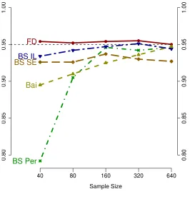
The results show that confidence sets for the Elliott and M¨uller approach, the

boot-strapped inverted LR approach, and the FD approach have good coverage accuracy across

different sample sizes. However, the expected length of the Elliott and M¨uller confidence set

is greater than the expected length for the FD or bootstrap inverted LR approaches. Also,

note that the ratio of lengths of the Elliott and M¨uller confidence sets to those of the

like-lihood based methods gets larger as the sample size increases. Strikingly, when the sample

size is 640, the Elliott and M¨uller confidence set is more than three times as long as that

of likelihood-based confidence sets. Bootstrap percentile and standard error confidence sets

have good coverage accuracy for large sample sizes such as 320 and 640, but they are also

longer than the FD and bootstrap inverted LR confidence sets. Meanwhile, the bootstrap

percentile and bootstrap standard error confidence sets do not have good coverage accuracy

for smaller sample sizes. Bai’s confidence intervals achieve relatively low coverage rates and

longer lengths, whereas the approach based on a bootstrap of Bai’s statistic brings out much

longer lengths without much improvement in terms of coverage rates.

4.2

A Structural Break in Variance

For a break in the variance of the error term, the model can be written simply as

yt=µ+et, et∼ i.i.d.N(0, σ_t2) (13)

where

σ_t2 =





 σ2

0 if 1≤t≤rT

σ2

1 if rT < t≤T ,

We set µ= 1, σ0 = 1, and σ1 = 0.5. The true break point fraction r is 0.5. The results are

presented in Figures 3(a) and 3(b).

Since an asymptotic distribution for a structural break in variance is not rigorously

0.80 0.85 0.90 0.95 1.00 0.80 0.85 0.90 0.95 1.00 FD Bai BS Bai BS Per BS SE BS IL Elliott& Mueller

40 80 160

Sample Size

320 640

(a) Coverage rates of confidence sets

Sample Size 40 010 30 50 BS Bai Bai Elliott& Mueller BS Per FD BS SE BS IL

Sample Size 80 010 30 50 BS Bai Elliott& Mueller BS Per Bai BS SE FD BS IL

Sample Size 160 010 30 50 BS Bai Elliott& Mueller BS Per Bai BS SE FD BS IL

Sample Size 320 010 30 50 Elliott& Mueller BS Bai BS Per Bai BS SE FD BS IL

Sample Size 640 010 30 50 Elliott& Mueller BS Bai Bai BS Per BS SE FD BS IL

(b) Average lengths of confidence sets

mean of the absolute values of errors from the regression model in (13) as in Stock and Watson

(2002) and Sensier and van Dijk (2004):

r π

2|et|=σ0(1−1[t > rT]) +σ11[t > rT] +ǫt.

The coverage rates of FD confidence sets are close to 95% over different sample sizes.

The bootstrap percentile and bootstrap inverted LR confidence sets have good coverage

accuracy for sample sizes larger than 160. However, the bootstrap percentile confidence sets

become much longer than those of the bootstrap inverted LR and FD methods as the sample

size increases. Meanwhile, the bootstrap standard error approach attains coverage rates well

below 95%, with relatively longer confidence sets compared to the FD and bootstrap inverted

LR approaches. The coverage rates of confidence sets based on Bai’s approach get close to

95% as the sample size increases, but the lengths are greater than those of confidence sets

based on other approaches, including being approximately twice as long as the confidence

sets based on the FD and bootstrap inverted LR approaches.

4.3

A Structural Break in Drift

For a break in drift in an otherwise trend stationary process, the model can be written as

yt=α+β0(t/T) +β1(t/T)1[t > rT] +et, et ∼i.i.d.N(0, σ2)

We set α = 1, β0 = 2, β1 =−0.5, and σ = 0.3. The true break point fractionr is 0.5. The

results are presented in Figures 4(a) and 4(b).

The bootstrap standard error approach and the likelihood-based approaches work well

with good coverage accuracy. The FD confidence sets have relatively short lengths for each

sample size. The confidence sets based on Bai’s asymptotic approach, the bootstrap of Bai’s

statistic, and the bootstrap percentile approach have coverage rates far below the nominal

95% level, with levels around 60% to 80% in sample sizes of 40 to 160. The confidence

sets based on the bootstrap of Bai’s statistic have relatively large expected lengths for each

0.80 0.85 0.90 0.95 1.00 0.80 0.85 0.90 0.95 1.00 FD BS Per

BS SEBS IL

Bai

40 80 160

Sample Size

320 640

(a) Coverage rates of confidence sets

Sample Size 40 0 20 40

Bai

BS Per

BS SE

FD BS IL

Sample Size 80 0 20 40

Bai

BS Per

BS SE

FD BS IL

Sample Size 160 0 20 40

Bai

BS Per

BS SE

FD BS IL

Sample Size 320 0 20 40

Bai

BS Per

BS SE

FD BS IL

Sample Size 640 0 20 40

Bai

BS Per

BS SE

FD BS IL

(b) Average lengths of confidence sets

0.6 0.7 0.8 0.9 1.0 0.6 0.7 0.8 0.9 1.0 FD Bai BS Bai BS Per BS SE BS IL

40 80 160

Sample Size

320 640

(a) Coverage rates of confidence sets

Sample Size 40 0 30 60 90 BS Bai BS Per BS SE BS IL FD Bai

Sample Size 80 0 30 60 90 BS Bai BS Per BS SE FD BS IL Bai

Sample Size 160 0 30 60 90 BS Bai BS Per BS SE FD BS IL Bai

Sample Size 320 0 30 60 90 BS Bai BS Per BS SE FD Bai BS IL

Sample Size 640 0 30 60 90 BS Bai BS SE BS Per Bai FD BS IL

(b) Average lengths of confidence sets

Table 1: Coverage rates and average lengths of confidence sets for the timing of two structural breaks in mean from Fiducial distribution approach based on Monte Carlo simulations

Fiducial Dist. 40 80 160 320 640 First Break 0.981 0.971 0.966 0.956 0.944

[16.09] [28.39] [45.46] [59.37] [65.53] Second Break 0.984 0.973 0.958 0.949 0.947

[16.03] [28.26] [45.84] [61.14] [64.70]

Notes: The coverage rates for confidence sets are constructed using a nominal 95% confidence level, with average lengths of the confidence sets reported in square brackets.

close to 95%, but it also produces confidence sets with relatively large expected lengths.

The bootstrap inverted LR approach has just below 95% coverage rate with relatively short

confidence sets.

4.4

Multiple Structural Breaks

For multiple structural breaks, we consider two cases: (i) two breaks in mean and (ii) one

break in mean and one break in variance, possibly at different break points. We examine the

performance of the FD approach only, as the Monte Carlo simulations for bootstrap methods

are computationally infeasible and Bai’s method has already been shown to perform poorly

in the case of only one break. In terms of implementation, the two break dates are sampled

from different blocks of the MH algorithm.

For case (i), the true DGP is as follows:

yt=µ0+µ11[t > r1T] +µ21[t > r2T] +et, et∼i.i.d.N(0, σ2),

We set µ0 = 1, µ1 =−0.5, µ2 = 0.5, and σ = 0.5. For the experiment, the true breakpoint

fractions r1 and r2 are 0.3 and 0.7, respectively. The results of Monte Carlo simulation are

summarized in Table 1. In finite samples, the true break dates are over-covered since the

minimum distance between two break dates increases the relative probabilities of allowable

break dates from what they would otherwise be. However, this effect disappears and the

coverage rates converge to the nominal 95% when the sample size is larger.

Table 2: Coverage rates and average lengths of confidence sets for the timing of one break in mean and one break in variance from Fiducial distribution approach based on Monte Carlo simulations

Fiducial Dist. Sample size 40 Breakpoint fraction r1 0.3 0.4 0.5

r2 0.7 0.6 0.5

Break in mean 0.964 0.955 0.948 [22.82] [21.93] [21.10] Break in variance 0.941 0.947 0.961

[20.51] [18.88] [17.92]

Notes: The coverage rates for confidence sets are constructed using a nominal 95% confidence level, with average lengths of the confidence sets reported in square brackets.

of one break in mean or variance. The true DGP is as follows:

yt=µ0+µ11[t > r1T] +et, et ∼i.i.d.N(0, σt2)

where

σ_t2 =





 σ2

0 if 1≤t≤ r2T σ21 if r2T < t≤T ,

We set µ0 = 1, µ1 =−0.5, σ0 = 1, and σ1 = 0.5. We perform three experiments by varying

true breakpoint fractions: a) 0.3 and 0.7, b) 0.4 and 0.6, and c) 0.5 and 0.5.14 _{The first break}

fraction in each experiment is for break in mean and the second is for break in variance. We

consider the sample size 40 only since the results of Monte Carlo simulations are similar to

those from one break in mean or variance. The results are summarized in Table 2. The

coverage rates are close to the nominal level 95%. Thus, when using the FD approach,

the existence of a break in mean does not materially affect the inference about a break in

variance and vice versa.

14

0.75

0.80

0.85

0.90

0.95

1.00

0.75

0.80

0.85

0.90

0.95

1.00

FD

Bai

BS Bai

BS Per

BS SE

BS IL E&M

0.3 0.4 0.5

True Break Date

(Sample size 40)

Figure 5: Coverage rates of confidence sets for the different timing of a break in mean

4.5

Robustness

Next, we examine whether the performance of FD approach is robust to the location of break

date or the presence of serially correlation.

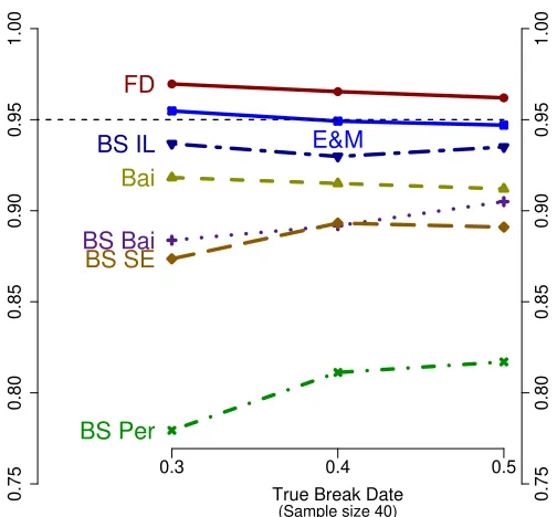
First, we vary the location of true breakpoint as a fraction of the sample from r= 0.3 to

0.5 in (12) for the case of a break in mean.15 _{The sample size is 40. Figure 5 presents the}

results. The coverage rates of confidence sets are robust to locations of true break dates. FD,

bootstrap inverted LR, and Elliott and M¨uller’s approaches result in coverage rates close to

95%.

Second, we generate serially correlated data with a structural break in mean. The true

DGP is as follows:

yt=µ0+µ11[t > rT] +ρyt−1+et, et∼i.i.d.N(0, σ2), 15

In the cases of r > 0.5, the Monte Carlo simulation results should be symmetric to the results when

0.75

0.80

0.85

0.90

0.95

1.00

0.75

0.80

0.85

0.90

0.95

1.00

E&M

FD

Bai

BS Bai

BS Per

BS SE BS IL

40 80 160

Sample Size

320 640

Figure 6: Coverage rates of confidence sets for a break in mean from serially correlated data

where µ0 = 1, µ1 = −0.5, σ = 0.5, r = 0.5 and ρ = 0.3. Figure 6 presents the results.

The coverage rates based on all the methods converge to 95% as the sample size increases.

However, in finite samples such as 40 and 80, only the FD and Elliott and M¨uller confidence

sets attain 95% coverage rates.

4.6

Summary of Monte Carlo Results

The main findings for the Monte Carlo analysis can be summarized as follows.

First, corresponding to their admissibility in the simple case of a break in mean with

known parameters, the likelihood-based confidence sets - i.e., those based on the FD and

bootstrap inverted LR approaches - produce the most accurate coverage rates and shortest

expected lengths in most cases. Furthermore, the ratios of the lengths of confidence sets

based on other approaches to lengths of the likelihood-based confidence sets become larger

as the sample size increases.

break dates. The fact that the coverage is so accurate directly implies that, in some way, the

marginal fiducial distributions provide good approximations of finite-sample distributions

that are close to being pivotal. Part of this accuracy could be because the nuisance

param-eters other than breakpoint paramparam-eters of our interest are integrated out of the likelihood

(for example, see Andrews and Ploberger (1994), Berger, Liseo, and Wolpert (1999), and

Elliott and M¨uller (2007)). However, the deeper question is what is it about the marginal

fiducial distributions that is essentially pivotal. Perhaps surprisingly, additional Monte Carlo

analysis reveals that various features of the marginal fiducial distributions are quite sensitive

to different parameter values. For example, we find that the relative height of the mode of

the fiducial distribution to the cut-off, k(1₋α), for including break dates in the confidence

set (a feature of the fiducial distribution that can be thought of as analogous to an LR

statistic), has a distribution across repeated samples that is highly dependent on the size

of the structural break. Instead, what appears to be more stable and explains the success

of the FD approach is the relative value of the cut-off k(1₋α) to the fiducial probability

of the true break date P r[τ = τ0]. In particular, the distribution of k(1−α)−P r[τ =τ0]

appears to always have an (1₋α) quantile equal to zero. To the extent that this quantile

is zero and higher quantiles are strictly positive, the FD confidence sets will have exactly

correct coverage. Of course, if the (1₋α) quantile were positive, the FD confidence sets

would under-cover because the cut-off k(1−α) would be above the P r[τ =τ0] in more than

α samples. On the other hand, if the (1₋α) quantile is zero, but some higher quantiles

are also zero, then the FD confidence sets would over-cover. Figure 7 reports Monte Carlo

results for the distributions of the differencek(1₋α)₋P r[τ =τ0] for different size structural

breaks in mean and for 1−α = 0.95,0.80, and 0.68. We find that, regardless of the size

of the break, the (1₋α) quantile is always exactly zero. When structural breaks are large,

some higher quantiles are also zero, so there is a tendency to over-cover in such cases.

How-ever, over-coverage in the case of very large structural changes is not particularly troubling

given that the only way to attain correct coverage in such a setting would be to have empty

confidence sets in α samples.

Third, some bootstrap methods perform very well in a sense of exact coverage in large

−1.0 −0.5 0.0 0.5 1.0

0.0

0.4

0.8

mu1= −0.5 (1−alpha)= 0.95 ECDF quantile( 0.95 )= 0

−1.0 −0.5 0.0 0.5 1.0

0.0

0.4

0.8

mu1= −0.5 (1−alpha)= 0.8 ECDF quantile( 0.8 )= 0

−1.0 −0.5 0.0 0.5 1.0

0.0

0.4

0.8

mu1= −0.5 (1−alpha)= 0.68 ECDF quantile( 0.68 )= 0

−1.0 −0.5 0.0 0.5 1.0

0.0

0.4

0.8

mu1= −1.5 (1−alpha)= 0.95 ECDF quantile( 0.95 )= 0

−1.0 −0.5 0.0 0.5 1.0

0.0

0.4

0.8

mu1= −1.5 (1−alpha)= 0.8 ECDF quantile( 0.8 )= 0

−1.0 −0.5 0.0 0.5 1.0

0.0

0.4

0.8

mu1= −1.5 (1−alpha)= 0.68 ECDF quantile( 0.68 )= 0

−1.0 −0.5 0.0 0.5 1.0

0.0

0.4

0.8

mu 1= −3 (1−alpha)= 0.95 ECDF quantile( 0.95 )= 0

−1.0 −0.5 0.0 0.5 1.0

0.0

0.4

0.8

mu 1= −3 (1−alpha)= 0.8 ECDF quantile( 0.8 )= 0

−1.0 −0.5 0.0 0.5 1.0

0.0

0.4

0.8

mu 1= −3 (1−alpha)= 0.68 ECDF quantile( 0.68 )= 0

the actual data are closer to the beginning or end of sample, the flipping in the percentile

bootstrap method produces very low coverage rates. This is because the parameter space

of interest (i.e., the possible break dates) is limited to 100 ×(1−2λ)% centered dates by

trimming as Π = [λT,(1₋λ)T] and some dates among potential break dates might not be

considered in the procedure to construct confidence set. In particular, suppose the true break

date is close to the first possible break date considered, λT _∈ Π. The number of periods

between the true break date and the first possible break date is very small and the number

of periods between the true break date and the ending break date (1₋λ)T is large. Then,

the two subsample periods before and after the estimated break date will be asymmetric. By

flipping, break dates that are estimated in the first subsample period area from bootstrapped

data sets will be used for bootstrapped distribution in the second subsample period, so that

the first subsample period cannot fully cover the second sub-interval, which is longer than

the first-sample period. By contrast, the second subsample period is flipped to cover the first

sub-interval, but some portion of the second subsample period might be out of the bounds

for possible break dates in Π. Thus, the bootstrap percentile methods may produce very

low coverage rates.16 _{When the sample size is very small, this problem arises even for the}

structural change at the middle point of the sample, r= 0.5.

Fourth, because Elliott and M¨uller (2007) use sequential tests to attain an exact coverage

rate, their test statistic is constructed in order to focus on producing the exact size of the test

rather than having high power to reject false break dates. Thus, their confidence sets may be

unnecessarily long.17 _{By contrast, since the FD approach relies on break date distributions}

conditional on the actual data, the confidence set for the FD method can be constructed

to be as short as possible, while maintaining an accurate coverage rate. In addition, if the

magnitude of the parameter change is very large, Elliott and M¨uller’s test easily rejects the

16

To illustrate, suppose the sample size is 40, the estimated break (ˆτ) is 10, and we have a 15% trimming rule for candidate break dates. Because we exclude the first 6 and last 6 points based on trimming, Π=[7,34]. Suppose the lower and upper bootstrap quantiles forτ∗b

−τˆare -3 and 24, respectively. The lower quantile is determined by the trimming rule. Then, the confidence set based on flipped quantiles would be [-14,13]. Thus, the trimming implicitly means that [14,34] will also be excluded from Π in practice and the coverage of the confidence sets based on flipping will be far below the nominal confidence level.

17

false hypotheses of break dates. Thus, in order to maintain correct coverage, all hypotheses

of break dates including the true break date will be rejected in α samples. That is, their

method can produces empty confidence sets, which are not particularly helpful inferences

when found or reported in a given empirical application (i.e., they are usually interpreted as

an indicator of model misspecification, even though this is not necessarily the case).

5

Application to Postwar U.S. Real GDP

5.1

Model Specification

We estimate break dates and model parameters by maximum likelihood estimation and apply

the various methods presented in section 2 in order to construct confidence sets for structural

breaks in postwar U.S. real GDP. In terms of our general model specification, we consider

the two possibilities that real GDP follows i) a nonstationary process with a unit root and

ii) a trend stationary process.

Under the assumption of a unit root, the model for M growth breaks and N variance

breaks is given as follows:

∆yt=c0+ M X

m=1

cmD(Tm) +

p X

j=1

φj∆yt−j +et, et∼i.i.d.N(0, σ2t) (14)

where σ2 t =                σ2

0 if 1≤t≤τσ2 1

σ2

1 if τσ2

1 < t≤τσ22 ...

σ2

N if τσ2

N < t≤T ,

and D(Tm) = 1 if t > τcm and 0 otherwise and τcm is mth break point for constant. The

lagged first differences account for serial correlation. We determine the number of first

difference terms, p, by the Schwarz Information Criterion (SIC).

We consider sequential asymptotic tests to determine the number and types of structural

breaks.18 _{The testing proceeds as follows: We begin with the null hypothesis of no structural}

18

breaks and the alternative of one break in constant or variance. If we can reject the null

hypothesis of no break, we assume one more break in the constant or variance and the

alternative hypothesis in the previous test becomes the null hypothesis in the new test. The

estimates of break dates in the alternative hypothesis from the previous test are maintained

and given in the null and the alternative for the new test and an additional break at an

unknown date is considered in the alternative. We keep performing these tests sequentially

until a null hypothesis cannot be rejected. In order to determine the number of breaks

and model specification, we consider LR statistics based on maximum likelihood estimates

under the null and alternative.19 _{The LR statistic is calculated from the log-likelihood}

values for the regression in (14). For example, suppose the null hypothesis regression hasM

breaks for constant and N breaks for variance and the alternative has M + 1 breaks and N

breaks, respectively. Then, given the number of break dates for the constant and variance

parameters, the particular break dates are chosen to make the LR test statistic from (14) as

large as possible and we reject the null hypothesis if this supLR test statistic is larger than

a specified critical value. Thus,

LR(τc0, . . . , τcM+1, τσ2₀, . . . , τσ2N)

=₋2_×[ logL(c0, . . . , cM, σ20, . . . , σ2N, φ1, ..., φp|y)

−logL(c0, . . . , cM+1, σ02, . . . , σN2, φ1, ..., φp|y) ]

{τcˆ1, ...,ˆτcM+1,τˆσ₁2, . . . ,τˆσ2_N}

= arg Max

τc₁,...,τ_cM+1∈Π, τ_σ2

1,...,τσN2∈Π

LR(τc1, . . . , τcM+1, τσ2₁, . . . , τσ_N2)

supLR statistic = val Max LR(ˆτc1, . . . ,τcˆM+1,ˆτσ12, . . . ,τˆσ2N)

Andrews (1993, 2003) provides tables of critical values for a supLR test of an unknown break

breaks. Levin and Piger (2007) use Monte Carlo analysis to show that this approach has good frequentist properties in finite samples. However, for simplicity, we focus on new techniques for making inferences about the timing of structural breaks, rather than inferences about their number and type.

19