NUMERICAL SOLUTION OF BLACK – SCHOLES PARTIAL DIFFERENTIAL EQUATION USING DIRECT SOLUTION OF SECOND - ORDER ORDINARY DIFFERENTIAL EQUATION WITH TWO - STEP HYBRID BLOCK METHOD OF ORDER SEVEN

(1)

Published by Faculty of Science, Kaduna State University

NUMERICAL SOLUTION OF BLACK – SCHOLES PARTIAL

DIFFERENTIAL EQUATION USING DIRECT SOLUTION OF

SECOND - ORDER ORDINARY DIFFERENTIAL EQUATION WITH

TWO - STEP HYBRID BLOCK METHOD OF ORDER SEVEN

1_{Olaiya O. O.,}2_{Oduwole H. K. and}3_{Odeyemi J. K.}

1_{Department of Mathematics,}_{Nasarawa State University, Keffi /NMC ABUJA.} 2_{Department of Mathematics,}_{Nasarawa State University, Keffi.}

3_{Department of Mathematics, University of Abuja.}

*Corresponding Author Email Address:[email protected]

ABSTRACT

This paper proposes a new numerical solution of Black-Scholes Partial Differential Equation using Direct solution of second-order Ordinary Differential Equation ODE with two-step hybrid Block Method of Order seven directly. The method is developed using interpolation and collocation techniques. The use of the power series approximate solution as an interpolation polynomial and its second derivative as a collocation equation is considered in deriving the method. Properties of the method such as zero stability, order, consistency, convergence and region of absolute stability are investigated The new method is then applied to solve Black –Scholes equation after converting it to the system of second-order ordinary differential equations and the accuracy is better when compared with the existing methods in terms of error.

Keywords: single-step; hybrid block method; system of second order ordinary differential equations; collocation and Interpolation method; direct solution.

INTRODUCTION

In the historical backdrop of option pricing model, the Black-Mcholes or Black –Scholes –Merton model is a standout amongst the most generous model. This model shows the significance role that the mathematics plays in the field of finance .

The Black – Scholes model was first published by Black and Scholes (1973) in their seminar paper “The Pricing of options and corporate Liabilities” published in the Journal of political Economy .In the same year, they derived a partial differential equation, now called the Black –Scholes Equation, which estimates the price of the option over time .

Let us consider 𝑆 as the price of the stock, which we consider as a random variable.𝑉(𝑠, 𝑡) be the value of an option as a function of time and stock price,𝐾, can be strike price,𝑟 be the risk –free interest rate ,𝜎 be the volatility/the standard deviation of the stock return ,and t be the time in years.Then the famous Black – Scholes equation that was developed by Fisher Black and Myron Scholes is

𝜕𝑉 𝜕𝑡+

1 2 𝜎

2_𝑆2 𝜕 2_𝑣

𝜕𝑆2+ 𝑟𝑆 𝜕𝑉

𝜕𝑆− 𝑟𝑉 = 0

The above equation is a second – order parabolic partial differential equation known as Black – Scholes equation ,is actually a variation of a famous equation in physics that models

the transfer of heat.

Simple Transformation of PDE to ODE

Black –Scholes equation is given by the following expression

𝜕𝑉 𝜕𝑡+

1 2 𝜎

2_𝑆2𝜕2𝑣 𝜕𝑆2+ 𝑟𝑆

𝜕𝑉

𝜕𝑆− 𝑟𝑉 = 0 (1)

where V(s,t) =price of option, σ is the volatility of stock price S, and V, t = period of time, r = interest rate (Company et al. , 2007). Firstly, it is expedient to transform this partial differential equation (PDE) into an ordinary differential equation (ODE) by proposing the following solution: V(S, t) = 𝑉(𝑆)𝑒𝜆𝑡_.

Given that 𝜕𝑉

𝜕𝑡= 𝑉(𝑆) ∗ 𝜆𝑒

𝜆𝑡_𝑎𝑛𝑑𝜕𝑉 𝜕𝑆=

𝜕𝑉(𝑆) 𝜕𝑆 𝑒

𝜆𝑡_,_by substituting these equations into the PDE, we get

𝑉(𝑆)𝜆𝑒𝜆𝑡₊1 2 𝜎

2_𝑆2𝑑2𝑉(𝑆)

𝑑𝑆2 𝑒𝜆𝑡+ 𝑟𝑆 𝑑𝑉(𝑆)

𝑑𝑆 𝑒 𝜆𝑡₋

𝑟𝑉(𝑠)𝑒𝜆𝑡_{= 0} ₍₂₎

The next step is to rearrange the equation to get second order ODE :

𝑒𝜆𝑡_[1 2 𝜎

2_𝑆2 𝑑2𝑉(𝑆) 𝑑𝑆2 + 𝑟𝑆

𝑑𝑉(𝑠)

𝑑𝑠 + 𝑉(𝑆)(𝜆 − 𝑟)] = 0. (3) The latter expression can be reduced to the following equation;

1 2 𝜎

2_𝑆2𝑑2𝑉(𝑆) 𝑑𝑆2 + 𝑟𝑆

𝑑𝑉(𝑠)

𝑑𝑆 + 𝑉(𝑆)(𝜆 − 𝑟) = 0 (4)

Where 𝑒𝜆𝑡_{≠ 0.}

Ordinary differential equations (ODEs)

Ordinary differential equations (ODEs) are commonly used for mathematical modelling in many diverse fields such as engineering, operations research, industrial mathematics, behavioural sciences, artificial intelligence, management and sociology. Thus, mathematical modelling is the art of translating problems from an application area into tractable mathematical formulations whose theoretical and numerical analysis provide insight, answers and guidance useful for the originating application. This type of problem can be formulated either in terms of first-order or higher-order ODEs.

In this Paper, the system of second – order ODEs of the following form is considered. We are interested in solving nonlinear time

Fu

ll L

en

gt

h Rese

ar

(2)

dependant PDE of the form [Black – Scholes Equation].

1 '' 1 1 1 ' 1 1 '

0 0 0 0

2 '' 2 2 2 ' 2 2 '

0 1 0 1

'' ' '

0 1 0

( ,

,

),

( )

,

( )

( ,

,

),

( )

,

( )

( ,

,

),

( )

,

( )

m m m m m m

n

y

f x y y

y x

a

y x

b

y

f x y y

y x

a

y x

b

y

f x

y

y x

a

y x

b



(5)

The method of solving higher-order ODEs by reducing them to a system of first-order equation involves more functions evaluation which to evaluate leads to computational burden as mentioned in (Master, 2011) and (Jator & Li. , 2012). The multistep methods for solving higher –order ODEs directly have been developed by many scholars such as (Yusuph & Onumanyi, 2005). However, these researchers only applied their methods to solve single initial value problems of ODEs.

The aim of this paper is to develop a new numerical method for solving single second – order ODEs and systems of second-order ODEs directly.

Derivation of the method

We shall be considering a two–step hybrid block method with five off step point, 𝑥_𝑛+1

3 , 𝑥_𝑛+2

3

, 𝑥𝑛+1, 𝑥𝑛+4 3

, 𝑥_𝑛+5 3

and 𝑥𝑛+2 for solving equation (5) is derived.

Let us consider the power series of the form

k_{𝑦(𝑥) = ∑} _𝑎

𝑖 𝑟+𝑠−1

𝑖=0 (

𝑥−𝑥𝑛 ℎ )

𝑖

, 𝑘 = 1, … , 𝑚 (6)

For 𝑥 ∈ [𝑥𝑛, 𝑥𝑛+1] 𝑤ℎ𝑒𝑟𝑒 𝑛 = 1,2, … , 𝑁 − 1, 𝑎𝑖, are real coefficients, r = the number of collocating points, s= the number of interpolating points and h = 𝑥𝑛+1− 𝑥𝑛 is a constant step size of the partition of the interval [a ,b] which is given by 𝑎 < 𝑥 < 𝑏; 𝑎 = 𝑥0< 𝑥1< 𝑥2< ⋯ , 𝑥𝑁−1 = 𝑏

Differentiating equation (6) twice give us

𝑦′′_{= ∑} 𝑖(𝑖−1)𝑎𝑖 ℎ𝑠 𝑟+𝑠−1

𝑖=0 (

𝑥−𝑥𝑛 ℎ )

𝑖−2

₍₇₎

Equation (6) can be resolved in form of approximate solution thus;

𝑦(𝑥) = ∑ 𝑎𝑖 𝑟+𝑠−1

𝑖=𝑜 𝑥𝑖

𝑦′(𝑥)_{= ∑ 𝑖 𝑎} 𝑖 𝑟+𝑠−1

𝑖=𝑜

𝑥𝑖−1

also,

𝑦′′_{(𝑥) = ∑ (𝑖 − 1)𝑖 𝑎} 𝑖 𝑟+𝑠−1

𝑖=𝑜

𝑥𝑖−2

where 𝑟 + 𝑠 − 1 = 7 + 2 − 1 = 8

Hence,

k_{𝑦(𝑥) = ∑} _𝑎

𝑖 8 𝑖=𝑜 𝑥𝑖 and

k_𝑦′′_{(𝑥) = ∑} _{(𝑖 − 1)𝑖 𝑎} 𝑖

𝑖=0 𝑥𝑖−2= f(x, y, y’)ℎ2

Now let us consider the point of interpolation at 𝑥_𝑛+1 3

𝑎𝑛𝑑 𝑥_𝑛+2 3 . Also, points of collocation belong to the interval [0, 2] i.e. 𝑥𝑛, 𝑥_𝑛+1

3 , 𝑥_𝑛+2

3

, 𝑥𝑛+1 , 𝑥_𝑛+4 3

, 𝑥_𝑛+5 3

and 𝑥𝑛+2.

Gives the following system of non -linear equation of the form:

2

2 2 2 2 2 2 2

2 2 2

1 1 1 1 1 1 1 1

1

3 9 27 81 243 729 2187 6561

2 4 8 16 32 64 128 256

1

3 9 27 81 243 729 2187 6561

2

0 0 0 0 0 0 0 0

2 2 4 20 10 14 56

0 0

3 27 27 81 729

2 4 16 160 160 448 3584

0 0

3 27 27 27 729

2 6 12 20 30 42 56

0 0

2 8 64 128

0 0

3

h

h h h h h h h

h h h 2 2 2 2

2 2 2 2 2 2 2

0 2560 14336 229376

27 27 81 729

2 10 100 2500 6250 43750 875000

0 0

3 27 27 81 729

2 12 48 160 480 1344 3548

0 0

h h h h

h h h h h h h

 

 

 

1

0 ₃

2 1

3

2

1 3

3

2 4

3

5 1

6 4

3

7 ₅

3

8

2

(8)

n n n

y a

f a

a f

a _f



    _ _   _ _   _ _   _   _   _   _   _   _  __   _   _   _   _   _   _   _   _   _   _   _ _

                

Solving equation (8) gives the coefficients 𝑎𝑖, 𝑖 = 0 , … ,8. Those values are then substitutes into equation (6) to gives Continuous hybrid multistep method of the form.

0

0 1

0

( )

k k

i n i

i

k k

i n n

i

y x

x y

y

x f

f





 

  

























V

V V

V

(9)

where k =2, 𝜈̅ =1 3 ,

2 3 , 1 ,

4 3 ,

5

3 yield the parameter 𝛼𝑖 and 𝛽𝑖, 𝑖 = 0, 𝜈̅, 1 as

𝛼_𝑛+1

3 = −3𝑡 + 2 𝛼_𝑛+2

3 = 3𝑡 − 1 where 𝑡 =𝑥−𝑥𝑛

ℎ So we have

(3)

2 6 7 2 8 3 5 4 0

2 8 7 6 5 4 3

1 3

2 8 7 6

2 3

21 459 27 1 81 863 49 441 203

32 4480 160 2 4480 108894 40 320 120

243 27 279 261 261 27623 8999

3

2240 28 80 40 40 60480 90720

243 513 1233 4149

896 224 160

h t t t t t t t t

h t t t t t t t

h t t t

      _         _       _        _  

    5 4 3

2 8 7 6 5 4 3

1

2 8 7 6 5 4 3

4 3

351 15 18689 769

320 32 4 120960 181440

81 81 363 279 127 10 139 1987

224 28 40 20 12 3 864 136080

243 459 963 2763 99 15 10921 1609

896 224 160 320 16 8 120960 1814

t t t t

h t t t t t t t

   _ _ _ _          _        _          

2 8 7 6 5 4 3

5 3

2 8 7 6 5 4 3

2

40

243 27 171 117 81 3 347 263

2240 35 80 40 40 5 12096 90720

81 27 51 27 137 1 479 221

4480 224 160 64 480 12 120960 544320

h t t t t t t t

            _        _      _        _   (10)

Evaluating the above continuous coefficients at 𝑡 = 0,1,4 3,

5 3, 2 (non-interpolating points), we obtain

Evaluating the above continuous coefficients at 𝑡 = 0,1,4 3,

5 3, 2 (non-interpolating points), we obtain

0 0 1 0

( )

k k

i n i

i

k k

i n n

i

y x

x y

y

x f

f





     

























V V V V V (11) 1 3 2

1 1 2 2 1

3 3 3

4 5 2

3 3 221 977 544320 90720 16451 1357 2 181440 136080

71 31 31

181440 90720 544320

n n

n _n _n _n n

n

n n

f f

y y y h f f

f f f

  _ _ _                                    (12) 1 3 2

4 1 2 2 1

3 3 3 3

4 5 2

3 3 137 209 181440 10080 433 4927 2 3 2240 45360

257 1 31

20160 672 181440

n n

n

n n n n

n

n n

f f

y y y h f f

f f f

           _ _                            (13) 1 3 2

5 1 2 2 1

3 3 3 3

4 5 2

3 3 19 17 181440 560 2987 4927 3 4 10080 22680

389 41 11

3360 5040 90720

n n

n

n n n n

n

n n

f f

y y y h f f

f f f

           _ _                            (14) 1 3 2

2 1 2 2 1

3 3 3

4 5 2

3 3 95 389 54432 9072 7085 4633 4 5 18144 13608

3893 1061 409 18144 9072 54432

n n

n _n _n _n n

n

n n

f f

y y y h f f

f f f

  _ _ _       _ _                            (15)

Differentiating (11) yields

' 1 1

0 1 1 1 0

1

( )

k

i n i n

i k

i n n

i

y x

x y

y

h

x f

f





         





















(16)

where ₁' ₂'

3 3

3

( )

t

,

( )

t

h











' 7 6 5 4 3 2

0

' 7 6 5 4 3 2

1 3

' 7 6 5 4 3 2

2 3

81 189 63 441 203 147 459 ( )

560 160 16 40 30 40 4480

243 27 837 261 261 27623

( ) 9

280 4 40 8 10 60480

243 513 3699 4149 351 45 1868 ( )

280 32 80 64 8 4

t h t t t t t t t

t h t t t t t t

      _        _       _       _         

' 7 6 5 4 3 2

1

' 7 6 5 4 3 2

4 3

' 7 6 5 4 3 2

5 3

9 120960 81 81 1089 279 127 139

( ) 10

28 4 20 4 3 864

243 459 2889 2763 99 45 10921 ( )

112 32 80 64 4 8 120960

243 27 513 117 81 9 ( )

280 5 40 8 10 5

t h t t t t t t

             _       _      _       _          

' 7 6 5 4 3 2

2

347 12096 81 27 153 135 137 1 479 ( )

560 32 80 64 120 4 120960

t h t t t t t t

          _       _   (17)

Evaluating equation (16) above at 𝑡 = 0,1 3,

2 3, 1,

4 3 ,

5 3 , 2

2 3

' 2

1 2 1 1 4 5 2

3 3 3 3 3

' 2

1 1 2 1 1

3 3 3 3

459 27623 18689 139 10921 347 479

3 3

4480 60480 120960 864 120960 12096 120960

199 1973 18 4157

3 3

72576 20160 128 90720

n _n _n n _n n n _n _n n

n n n

n n n n

hy y y h f f f f f f f

hy y y h f f f f

                   _       _         2 3

4 5 2

3 3

' 2

2 1 2 1 1 4 5 2

3 3 3 3 3 3

' 2

1 1 2

3 3

851 41 289

40320 6720 120960

731 13 6347 3971 257 109 253

3 3

362880 320 40320 90720 13440 20160 262880

1

3 3

1920

n

n n

n n n n

n n n n n n

n n

f f f

y y y h f f f f f f f

hy y y h f

             _ _                _       _   

   2

3

2 3

1 1 4 5 2

3 3 3

' 2

4 1 2 1 1 4 5

3 3 3 3 3 3

1537 39587 4927 2201 209 43

60480 120960 30240 120960 6720 120960

571 691 1299 33533 1223 79

3 3

362880 20160 4480 90720 8064 6720

n n

n

n n n

n n n n n n

f f f f f f

hy y y h f f f f f f

               _ _ _ _ _ _                2 3 2 ' 2

5 1 2 1 1 4 5 2

3 3 3 3 3 3

' 2

2 1 2 1

3 3 3

59 51840

29 51 13313 5081 5519 73 1313

3 3

362880 2240 40320 18144 13440 576 362880

13 3481 5293

3 3

2688 60480 24193

n

n n n n

n n n n n n

f

hy y y h f f f f f f f

hy y y h f f f

           _ _ _             _       _   

     2

3 1 4 5 2

3 3

14719 2671 29369 12287

30240fn 17280fn 576 fn 120960fn

  

 

   

 

(4)

Equation (9) is evaluated at non-interpolating points, i.e, 𝑥𝑛, 𝑥_𝑛+1

3 , 𝑥_𝑛+2

3

, 𝑥𝑛+1 , 𝑥_𝑛+4 3

, 𝑥_𝑛+5 3

and 𝑥𝑛+2, while Equation (16) is evaluated at all points, and this yields the following equation in matrix form:

1 2 3

m

A





BR



CR



DR

(19)

Where

*

2 1 0 0 0 0 0 0 0 0 0 0

1 2 1 0 0 0 0 0 0 0 0 0

2 3 0 1 0 0 0 0 0 0 0 0

3 4 0 0 1 0 0 0 0 0 0 0

4 5 0 0 0 1 0 0 0 0 0 0

3 3

0 0 0 0 0 0 0 0 0 0

3 3

0 0 0 0 1 0 0 0 0 0

3 3

0 0 0 0 0 1 0 0 0 0

3 3

0 0 0 0 0 0 1 0 0 0

3 3

0 0 0 0 0 0 0 1 0 0

3 3

0 0 0 0 0 0 0 0 1 0

3 3

0 0 0 0 0 0 0 0 0 1

h h A h h h h h h h h h h h h     _                       _    _        1 3 2 3 1 4 3 5 3 2 ' 1 3 ' 2 3 ' 1 ' 4 3 ' 5 3 ' 2 , (20) n n n n n n m n n n n n n y y y y y y y y y y y y                                                     _     1 ' 1 0 0 0 0 0 0 0 0 0 0 1 , , 0 0 0 0 0 0 0 0 0 0 0 0 n n y B R y               _ _   _ _   _ _   _ _   _ _   _ _   _ _   _  _      _ _   _ _   _ _   _ _   _ _   _ _   _ _   _ _   _ _              

 

2 2 2 2 2 2 863 108864 221 544320 137 181440 19 1881440 95 54432 459 4480 , , 199 72576 731 362880 1920 571 362880 29 362880 13 2688 n h h h h h h

C R f

h h h h h h                                                      _       _       _      _      1 3 2 3 1 3 4 3 5 3 2 2 2 , 8999 769 90720

(21)

n n n n n n f f f R f f f h h D                                       

2 2 2 2

2 2 2 2 2 2

2 2 2

1987 1609 263 221

181440 136080 181440 90720 544320

977 16451 1357 71 31 31

90720 181440 136080 181440 90720 544320

209 433 4927 257 31

10080 2240 45360 20160 672 181440

17 2987 4927

560 10080 22

h h h h

h h h h h h

h h h

 



2 2 2

2 2 2 2 2 2

389 41 11

680 3360 5040 90720

389 7085 4633 3893 1061 409

9072 18144 13698 18144 9072 54432

27623 18689 139 10921 347 479

60480 120960 864 120960 12096 120960

1973 18 4157 851 41

20160 128 90720 40320 6720

h h h

h h h h h h

h h h h h



 

   289

362880

13 6347 3971 257 109 253

320 40320 90720 13440 20160 262880

1537 39587 4927 2201 209 43

60480 120960 30240 120960 60480 120960

691 1299 33533 1223 79 59

20140 4480 90720 8064 6720 51840

51 13313

2240 4032

h

h h h h h h

h

h h h h h h

h h



 



5081 5519 73 1313

0 18144 13440 576 362880

3481 5295 14719 2671 29369 12287

60480 24192 30240 17280 60480 120960

h h h h

h h h h h h

                                                           _           

Multiplying equation (19) by 𝐴−1_{gives the hybrid Block method} as shown below

* * *

1 2 3

m

I





B R



C R



D R

(22)

(5)

* 1 3 2 1 3 1 1 0 0 0 0 0 0 0 0 0 0 0

0 1 0 0 0 0 0 0 0 0 0 0

0 0 1 0 0 0 0 0 0 0 0 0

0 0 0 1 0 0 0 0 0 0 0 0

0 0 0 0 1 0 0 0 0 0 0 0

0 0 0 0 0 1 0 0 0 0 0 0 , 0 0 0 0 0 0 1 0 0 0 0 0

0 0 0 0 0 0 0 1 0 0 0 0

0 0 0 0 0 0 0 0 1 0 0 0

0 0 0 0 0 0 0 0 0 1 0 0

0 0 0 0 0 0 0 0 0 0 1 0

0 0 0 0 0 0 0 0 0 0 0 1

h h h I B                      _ _                    2 2 2 2 2 2 * 28549 1088640 1027 17010 253 2688 1088 4 1 8505 3 177151 5 1 1088640 3 41 1 2 210 , 19087 0 1 181440 1139 0 1 11340 137 0 1 1344 2 0 1 0 1 0 1 h h h h h h h h C h h h                  _              _        _                          _       _      , 86 2835 3715 36288 41 420 h h h                                                                      

2 2 2 2 2 2

2

*

275 5717 19621 7703 3991 199

5184 120960 272160 362880 120960 217728

194 8 788 97 11447 19

945 81 8505 1890 181440 8505

165 2

448

(23)

h h h h h h

h D          

2 2 2 2 2

2 2 2 2 2 2

2 2 2 2 2

67 5 363 419 47

4489 32 4480 4489 13440

1504 8 2624 8 539 8

2835 945 8505 81 4320 1701

8375 3125 25625 625 10541 1375

12096 72576 54432 24192 72576 217728

6 3 68 3 149

0

7 35 105 70 2240

166

h h h h h

h h h h h h

h h h h h

  

   

  



771 35699 586 523 10183 41

30240 120960 2835 7560 120960 12960

94 11 332 269 10267 595729

189 3780 2835 3780 120560 198737280

27 387 34 243 10921 29

56 2240 105 2240 120960 6720

464 128 1504 58

945 945 2835 945

h h h h h h

h h h h

           2 2 12343 8 120960 2835

725 2125 250 3875 4409 275

1512 12096 567 12096 120960 36288

18 18689 5293 139 14719 9 253 41

35 18689 24192 864 30240 140 640 420

h

h h h h h h

h h h h h h h h

                                                  _    _    _                

The above blocked method is of uniform order 𝑃 = (7,7,7,7,7,7,7)𝑇_{with an error constant}_𝑐

𝑝+2

Analysis of the method

Zero stability

The two step hybrid block method (Jator, 2013) is said to be zero stabile if no root of the first characteristic equation 𝜌(𝑅) has modulus greater than one ,i.e |Rm|≤ 1 and if Rm =1,then the

multiplicity of Rm must not exceed 2.

The characteristic function of the new derived method is given as below;

0 0 0 0 0 0 0 0 0 0 0

( )

0 0 0 0 0 0 0 0 0 0 0

0 0 0 0 0 1 0 0 0 0 0

R h                                _ _                   3 2

0 0 0 0 0 1 0 0 0 0 0

3

0 0 0 0 0 1 0 0 0 0 0

4

0 0 0 0 0 1 0 0 0 0 0

3 5

0 0 0 0 0 1 0 0 0 0 0

3

0 0 0 0 0 1 0 0 0 0 0 2

0 0 0 0 0 0 0 0 0 0 0 1

h h h h h                                                           

0 0 0 0 1 0 0 0 0 0

3 2

0 0 0 0 1 0 0 0 0 0

3

0 0 0 0 1 0 0 0 0 0

4

0 0 0 0 1 0 0 0 0 0

3 5

0 0 0 0 1 0 0 0 0 0

3

0 0 0 0 0 1 0 0 0 0

(24) h h h h h                         

 0 2

0

0 0 0 0 0 0 0 0 0 0 1

0 0 0 0 0 0 0 0 0 0 0 1

(6)

Thus, . 𝜆10_{(𝜆 − 1)}2_{= 0} ₍₂₅₎

Where 𝜆𝑖 ={_{1 𝑖𝑓 𝑖 = 11,12.}0 𝑖𝑓 𝑖 = 1(1)10 (.26)

Hence, the developed method is zero stable.

Order of the method.

According to Yusuph & Onumanyi (2005) the order of the new method in equation Leentvaar (1973) is obtained by using the Taylor series and it is found that the developed scheme has an order of (7,7,7,7,7,7,7)𝑇_{with an error constant vector of;} [1.732063 ×10−7_{, 4.1014112 ×}₁₀−7_{, 6.582812 ×}₁ 0−7_{, −1.745322 ×}₁₀−6_,

1.531063 ×10−7_{, 1.732063 ×}₁₀−6_{, −1.666063 ×}₁₀−5_]

Consistency

Hybrid block method is said to be consistent if it has an order that is more than or equal to one. The order is order two. Therefore, the method is consistent.

Convergence

Zero stability and consistency are sufficient conditions for a linear multistep method to be convergent (Onumanyi, 1981). Since the new hybrid block method is zero stable and consistent, it can be concluded that the method is convergent.

Implementation of the Method

The initial starting value at each block is obtained by using Taylor series method. Then, the outcomes are calculated and corrected using the new scheme. For the next block ,the same technique are repeated to compute the approximate values of 𝑥_𝑛+1

3 , 𝑥_𝑛+2

3 , 𝑥𝑛+1, 𝑥𝑛+4

3

𝑎𝑛𝑑 𝑥_𝑛+5 3

until the end of the integrated intervals .During the calculations of the iteration, the final value of yn+1 are

taken as the initial values for the next iteration.

Numerical Experiment/Result

In this section, the performance of the developed two step hybrid block scheme is examined. The tables below shows the numerical results of the new developed scheme with exact solution for solving the problem and the result of the developed scheme are more accurate than that of Dura & Osneagu (2010) which was executed by six step method for solving the equation

Problem: Consider for purposes solving for the value of call option with strike price k=100. The risk – free interest rate r = 0.12, the time to expiration is T = 1 measured in years, and the volatility is = 0.10.The value of the call option can have a range of 70≤ 𝑠 ≤ 130.

Table 1. Comparison between the explicit method and Hybrid method

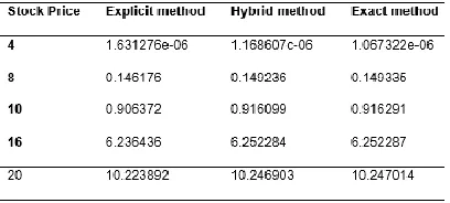
Table 2. .Approximate value by hybrid method and the exact value

Comparison with Other Numerical Scheme

In this part, a comparison is made between our Hybrid Scheme with another scheme that was used in finding the approximate solution of Black- Scholes model which is explicit method For a European call option with 0 ≤ 𝑆 ≤ 20,𝑇 = 0.25, 𝑘 = 10, 𝑟 = 0.1, 𝜎 = 0.4, with temporal grid size of N= 2000 and spatial grid size 𝑀 = 200, the explicit method and Hybrid method were used to set the table above.

From Table 1,it is seen that hybrid scheme gives better results than explicit method .But the results obtained by the scheme that was developed here are not much close to the exact value .But the good news is that if the temporal grid points are increased up to 𝑁 = 41000, spatial grid points up to 𝑀 = 1000 and set the other parameters value as above, then the following value (Table 2) were found much more better for different stock prices. The numerical result confirm that the proposed scheme produces a better accuracy if compared with the existing methods

Conclusions

In this article, a two-step block method with five off-step points is derived via the interpolation collocation approach. The developed method is consistent, Zero Stable, Convergent and of order seven. The relative error of the hybrid scheme was estimated by comparing the numerical solution with the analytical solution in Li-norms. The numerical simulation results are seen in good agreement with well- known qualitative behavior of the Black Scholes PDE .Also,a comparison is presented between the hybrid method and the result obtained by another work using the explcit method where our result is found more accurate than that of the explicit method.

Conflicts of interest: The authors declare no conflict of interest.

REFERENCES

Awoyemi, D.O. et al. (1994). New linear Multistep methods with Continuous Coefficients for first order IVP.J.Nig.Math.Soc.13, pp 383 – 400.

Back, F. and Scholes, M. (1973). ‘The pricing of options and corporate liabilities”, Journals of politica Economy,637- 654.

Bahi, C. (2007). Modelos de medicion de la Volatilidad en los mercados de valores;Aplicacion al Mercado bursatil argentine Universidad Nacional de Cuyo,Facultad de acciones.

Company R, Gonzalez ,A.L. and Joder L. (2007). Numerical

solution of Modified Black –Scholes Equation

(7)

Pricing Stock Option with Disccrete Dividend. Mathematics and Computer Modeling.44.1058-1068.

Dura,G. and Osneagu, A.M. (2010). Numerical Approximation of Black –Scholes Equation .An.Stiint University.” Al.I Cuza” Iasi,Mat,56, 39-64.

Fatunla, S.O. (1999). Block Methods for second – order IVP, Int .J.Mathematics 41(9) pp. 55 -63.

Jator, S.N. and J. Li (2012). An algorithm for second order initial and boundary value problems. Numerical Algorithm ,59.

Jator, S.N. et al. (2013). Stabilized Adams Type Method with a Block extension for Valuation of options. Ninth MSU-UAB conf.

Jodar, L. ,Sevilla-peris, P.,Cortes,J.C. and Sala, R. (2015). A New Direct Method for Solving The Black –Scoles Equation.

Applied Mathematics Letters.18,29,-32.

Lambert,J.D. (1973). Computational Methods in ODEs :John Wiley and Sons;New York, NY,USA.

Leentvaar C.C. (2003). “Numerical Solution of the Black-scholes Equation with a small Number of Grid Points ”Delf University of Technology. (A Master’s Thesis).

Manabu K. (2008). “On the Black scholes Equation; Various Derivation”MS&E.408 Term paper.

Master ‘O’Equity Asset Manegement@2006-2011 “Black scholes Model” Retrieved From www.optiontradingpedia.com on 28TH_{September, 2011.}

Onumany, P. (1981).Numerical Solution of B.V.Ps with the Tau Method, Phd Thesis University of London,England.

Paolo Brandimarte (2006). “Numerical Methods in Finance and Economics” 2nd_{edition. John Wiley &Sons, inc. Hoboken}

New Jersey.