R E S E A R C H
Open Access
Detection and tracking of moving objects in a
maritime environment using level set with
shape priors
Duncan Frost and Jules-Raymond Tapamo
*Abstract
Over the years, maritime surveillance has become increasingly important due to the recurrence of piracy. While surveillance has traditionally been a manual task using crew members in lookout positions on parts of the ship, much work is being done to automate this task using digital cameras coupled with a computer that uses image processing techniques that intelligently track object in the maritime environment. One such technique is level set segmentation which evolves a contour to objects of interest in a given image. This method works well but gives incorrect
segmentation results when a target object is corrupted in the image. This paper explores the possibility of factoring in prior knowledge of a ship’s shape into level set segmentation to improve results, a concept that is unaddressed in maritime surveillance problem. It is shown that the developed video tracking system outperforms level set-based systems that do not use prior shape knowledge, working well even where these systems fail.
Keywords: Tracking; Level sets; Shape priors; Maritime surveillance
1 Introduction
While the word ‘pirate’ brings to mind thoughts of the swashbuckling, one-eyed seafarers of childhood fantasy, the term still, unfortunately, has use in today’s modern world. Costing an estimated US$13 to 16 billion a year [1], piracy remains a pertinent problem in areas such as the coast of Somalia and the Gulf of Guinea. Despite increased security, piracy in these areas is increasing over the years. While recent years have seen a slight drop in reported incidents of piracy, 439 attacks were reported in 2011 according to the International Maritime Bureau [2].
Due to the increased threat of piracy, surveillance is an absolute must on cargo ships travelling in these danger-ous areas. While radar systems have been extensively used in maritime environments, these generally require large, metallic targets. Modern pirates favour small, fast rigid inflatable boats that are mainly non-metallic and thus difficult to detect [3]. While the solution to this would seem to be the use of manual detection using dedicated crew members on board, the small number present at any given time makes this unfeasible. Unlike humans that
*Correspondence: [email protected]
School of Engineering, University of KwaZulu-Natal, Durban 4041, South Africa
grow tired, automated video surveillance systems are able to constantly monitor camera feeds and keep track of a number of objects of interest around the ship.
Szpak and Tapamo [4] present an approach that at-tempts to track objects using a closed curve in the image (a method known as level set segmentation) after they had been detected using a motion-based detection sys-tem. While the tracking results are very good, object detection suffers from detection of a large number of non-ship objects due to motion from waves. To address these shortcomings, this work investigates the possibil-ity of integrating prior-known shape information into segmentation.
The rest of the paper is structured as follows: Section 2 covers the background on level set methods and their implementation and reviews the theory associated with shape priors. Section 3 discusses applications of image processing and level sets within the maritime surveil-lance environment. Section 4 introduces the proposed video tracking system and details various subsystem func-tionalities. The various subsystems are implemented in Section 5, and the final system is established. Section 6 concludes and outlines future work.
2 Background
There have been a number of attempts to address the problem of detecting and tracking objects at sea. Some of the main tasks to achieve this goal are understanding of the nature of the sea clutter and its modelisation for accurate segmentation of moving objects.
In [5], temporal characteristics of sea clutter and that of a range of small boats are analysed using a comprehen-sive set of recorded datasets. This is done in an attempt to understand the dynamics and associated reflexivity of small boats. An empirical sea model is then derived. It then allows the development of advanced detection and tracking algorithms, which will help improve the perfor-mance of surveillance and marine navigation radar against small boats.
Vicen-Bueno et al. [6] propose neural networks-based signal processing techniques to reduce sea clutter. In [7], several machine vision techniques that could help in eas-ing the search tasks in maritime environment are investi-gated. Hidden Markov model-based tracking models are then used to design a system that improves detection performance.
In this paper we propose an approach to ship detec-tion and tracking based on active contours. Active contour methods are segmentation techniques that use an iter-atively evolving contour or interface in an image that separates different regions of interest. Active contours can be expressed using one of two principle approaches [8]:
• Explicit or Lagrangian approach resulting in an interface known assnake.
• Implicit or Eulerian approach resulting in an interface called alevel set.
Kass et al. [9] initially introduced the concept of active snakes for expressing the contour in an image in which a parameterised spline is guided in the image to a desir-able position by a number of forces. The major problem with active snakes is its inability to deal with changes in topology [10]. Closed contours expressed as active snakes are unable to deal with splitting or merging of regions in
an image. Level set methods were originally introduced by Osher and Sethian [11] as a method to evolve a con-tour with a speed proportional to its curvature. The main advantage of this method is that, unlike active contours, it allows for cusps, corners and automatic topological changes [10].
Given an imageI(x,y), where(x,y) are image coordi-nates, a three-dimensional surface defined by a level set function(x,y)is defined on top of it. The contourCis in the image and implicitly defined as the zeroth level set (hence the name) of the level set functionφ:
C= {(x,y)|φ (x,y)=0}. (1)
To visualise this expression, see Figure 1 where a con-tour in the image shown in Figure 1a is defined as part of the image in Figure 1b that is cut by the level set surface at
=0 .
To ensure a one-to-one mapping between the level set function and its corresponding contour, the level set func-tionis constrained to a signed distance function, that is, |∇| =1 almost everywhere with >0 inside the con-tour and <0 outside the contour [12]. Informally, this can be thought of as the distance to the zero-level contour inside the contour and its additive inverse outside.
2.1 Chan-Vese energy functional
The original implementation introduced in [11] attempts to simulate active snake behaviour using a level set func-tion’s contour. The contour is evolved according to active-snake-like forcesFin the normal direction to the contour (in the image) to simulate the behaviour of active snakes. To do so,the following differential equation is used:
∂
∂t =F|∇| (2)
Rather than using a predefined set of forces in the image, variational level set methods seek to produce a level set function that minimises a predefined cost function, more specifically known as energy functional also sometimes called acost functional.
Chan and Vese introduce a regional-based variational formulation in [10] that is designed to work with images without edges byminimising the variation in pixel inten-sity inside and outside the contour. The expectation is to move the level set contour around an image segment that is homogenous with respect to pixel intensity. The Chan-Vese energy consists of two internal energies,Elength and Earea, that penalise the length of the contour and the area within it respectively (therefore favouring small, short contours) and two external energies,Evar_insideand
Evar_outside, that penalise variation in pixel intensity inside the contour and outside the contour respectively:
Ecv= =μElength+νEarea+λ1Evar_inside+λ2Evar_outside, (3)
whereμ,ν,λ1andλ2are parameters weighting the impor-tance of their respective penalty terms. The contour needs to be evolved untilEcvis minimised.
Given an image,I, with its domain, the inner and outer pixel variation terms can be expressed as
Evar_inside=
|
I−c1|2H()dx. (4)
Evar_outside=
|
I−c2|2(1−H())dx, (5)
whereHis the Heaviside function defined as
H(x)=
1 ifx≥0
0 ifx<0. (6)
In a level set formulation, the Heaviside function is used to specify areas inside the contour, whereH()=1 , and outside the contour, 1−H() = 1. The valuesc1 and
c2are the average pixel intensities inside and outside the level set contour respectively calculated as
c1()=
ωI×H()dx
H()dx
. (7)
c2()=
ωI×(1−H())dx
(1−H())dx
. (8)
The resulting evolution equation that minimises the functional in Equation 9 is as follows:
∂
∂t =δ()
μdiv
∇
|∇|
−ν−λ1(I−c1)2+λ2(I−c2)2
.
(9)
2.2 Level sets with shape priors
Shape priors can be very useful in segmentation, mainly when the object to be segmented is corrupted. This is often the case in real-world applications, such as mar-itime surveillance. In [13], it is shown how an object partially occluded can be accurately segmented. Adding
shape knowledge can be achieved by modifying a vari-ational energy functional designed for segmentation by adding an additional term that penalises deviation from a particular shape.
The majority of techniques that incorporate shape pri-ors use a linear combination of two functionals with one as a common segmentation functional (as discussed in Equation 9) and the other a shape difference [14]. The pur-pose of the shape difference term is to penalise level set contours that deviate from a predefined shape. A rudi-mentary example introduced by Rousson and Paragios [15] is the squared difference between the segmenting level set function and a predefined level set function that incorporates the desired shape:
Eshape(,)=
((x)−(x))2dx. (10)
The term in Equation 10 is added to the segmentation-based term (such as Chan-Vese). It is often multiplied by a weighting factorαto control the balance between the two terms:
E(,)=Ecv()+αEshape(,). (11)
Parametric methods of incorporating shape informa-tion impose this knowledge directly into the level set by defining the level set as the output of some parametric function and minimising segmentation energy functionals with respect to these parameters. Tsai et al. [16] introduce a parametric level set function that is an affine trans-formed version of a prior-known shape, defined in a level set function , for the use of shape priors. Parameters controlling translation, scale and rotation of the origi-nal shape are then optimised, rather than the level set function.
The use of multiple shape priors is documented in the literature and involves the use of selective and compet-ing shape priors. Tsai et al. [16] propose expresscompet-ing a level set function as a parametric combination of the principle components from a set of training shapes. In [15,17], the authors create a model of a set of prior shapes by assuming that shape priors follow pixel-wise Gaussian distributions. Cremers et al. [18] implement a shape model using a ker-nel density estimator to produce a statistical shape model that can model fairly distinct training shapes. A shape dis-tance measure is then defined based on Chan and Zhu’s work [14].
3 Image processing approach to ship tracking 3.1 Traditional approach
producing erroneous detection with methods that detect moving objects, some authors choose to characterise it and label pixels that do not match this characterisation as objects of interest. Sanderson et al. [3] implement an algorithm that does this using frequency information. Smith and Teal [19] implement a similar approach using a histogram-based descriptor of the appearance of the sea. Voles and Teal [20] propose a method that is based on the use of crude descriptors of tiles in an image; the image is divided into overlapping tiles that increase in size as they get closer to the bottom of the image. This method often results in imprecise segmentation results. Voles et al. [21] improve the method presented in [20] by adding motion information obtained using frame differencing; the algo-rithm designed is purely pixel-based and therefore fails to segment larger maritime objects.
Gupta et al. [22] describe the development of the Mar-itime Activity Analysis Workbench; this project aims at overcoming limitations of the current maritime surveil-lance systems. In [23], Ponsford et al. present the design and implementation of an integrated maritime surveil-lance system based on high-frequency surface wave radars. Leung et al. [24] combine genetic algorithm and radial basis function neural network to search optimal val-ues of a detector model. This model is then used to detect small surface targets in various sea conditions. In [25], an estimation of the ship size using an ANN-based clutter reduction system is proposed.
Socek et al. [26] present a method of combining exist-ing object detection methods with colour information. It initially segments the foreground using background mod-elling with a Bayes decision framework that works best for backgrounds with complex variations and that are not periodic. In a maritime environment, the algorithm suffered from poor segmentation results having inaccu-rate boundaries and many scattered pixels. The authors seek to solve these issues by combining results with that of colour-based segmentation. Colour segmentation is treated as a graph-partitioning problem, and combining it with background subtracted output results in enhanced performance. There have also been many other attempts to build maritime surveillance systems; some example could be found in [27,28].
3.2 Level set approach
Szpak and Tapamo [4] introduce an approach that uses level set methods as a way to track detected maritime objects in a scene. Object detection is implemented using a modified method of single Gaussian background sub-traction. Where normal background subtraction deals with pixels in isolation, spatial-smoothness constraint is enforced to deal with neighbourhoods of pixels. The straint assumes that real-world objects are spatially con-sistent entities and requires that a whole group of pixels,
rather than single ones, exhibit motion behaviour before marking them as such. The output of this method is fur-ther segmented using level set methods. The contour is used in the tracking phase as described by Bertalmio et al. [29], where the final contour from the previous frame is used as an initial contour in the next. The algorithm was tested in 17 test sequences and showed promising results. It was able to successfully track in all but three of the 17 given sequences. The algorithm even showed good results in overcast and rainy conditions. It failed in sequences where there was insufficient contrast between the ocean and the target and thus fails to pick up specific motion of the target, when the target moves too slowly and is thus considered part of the background and when there is a lot of glint in the scene. Due to its high success rate and possible avenues for improvement, it was decided to base further work on the model proposed in [4].
4 Proposed model of ship tracking using level sets with shape priors
The fundamental contribution of the work presented in this paper is the proposition of a method of incorporating shape knowledge into the system discussed in [4].
4.1 Model overview
Figure 2System overview.
The input to the system is a sequence of grey scale image frames from a video of a maritime scene. The output of the system is ideally the same set of image frames with various maritime objects of interest highlighted by a level set contour. An overview of how the system functions is as follows:
• The object tracker does not run until it has received a set of initial object positions from the object detector.
• The object detector uses a background subtraction algorithm that only uses input frames periodically at a fixed spacing. Only once it is filled a buffer of frames is it able to produce an output, and so until then the tracker, and thus the system, has no output. • Once the buffer is full, the detector is able to output a
set of objects to the tracker.
• Once it has obtained a set of initial object positions, the object tracker continues to track these objects.
The object detector is consist of a pre-filtering stage, followed by a background subtraction algorithm. The resultant binary images are then filtered again in a post-filtering algorithm to remove false positives in the image. If it is desired to find a particular shape that is known
beforehand, binary level set shape prior segmentation can be further applied in a level-set-filtering algorithm before the input to the object tracker.
The object tracker extracts features of the detected objects in the first frame after detection to create a model for each object. For each subsequent frame, the level set tracking algorithm uses this Figure 3 model, combined with its shape, to track the object. This information is fed back into the tracker for use in tracking the object in the next frame.
4.2 Level set segmentation algorithm
While Szpak and Tapamo [4] used a general level set seg-mentation algorithm based on the work of Chan and Vese in [10], the work presented here deals with incorporating shape knowledge into the system. There is then a need for a different method to introduce shape priors.
4.2.1 Level set algorithm of Tsai et al.
The system to be designed is based on the work of Tsai et al. [16]. The method presented in this work is based on a parametric function, which offers a number of benefits:
• Parametric models allow for a faster evolution that is less prone to getting stuck in local minima as the
energy is minimised directly by manipulating a few parameters rather than the entire contour. • Parametric models do not require function
re-initialisation. The resultant segmenting level set function is always a transformed version of an original signed distance function, which itself is thus a signed distance function.
• The limited degrees of freedom allows for more ‘brute force’ numerical methods of energy optimisation, which allow the contour to evolve according to any arbitrary energy functional without the need for symbolic differentiation.
Tsai et al. [16] deal with the incorporation of multi-ple shape priors in segmentation. For simplicity, however, the system described in this paper has been designed to use a single shape prior. For each sequence that is tested, the desired shape prior is manually set to the shape of an object that appears in that sequence. Simplification to a single shape prior allows the level set function to be manipulated using a set of pose parameters only (i.e. the one shape is known in advance and is given by the shape prior).
The set of pose parameters represented by the vector p=[a,b,h,θ]Tis introduced, whereaandbcontrol hor-izontal and vertical translation, h controls the scaling, andθ controls the rotation. The level set function can be parameterised in terms of these pose parameters. Con-sider a level set functionthat has a contour in the form of the desired shape prior. The level set functioncan be defined as a translated, scaled and rotated version of this original function:
[p](x,y)=(x,y), (12)
wherexandyare calculated according to ⎡
⎣xy 1
⎤ ⎦=T[p]
⎡ ⎣xy
1 ⎤ ⎦
= ⎡ ⎣1 00 1ab
0 0 1 ⎤ ⎦
M(a,b) ⎡ ⎣h0 0 0h0
0 0 1 ⎤ ⎦
H(h) ⎡
⎣cossin(θ )(θ )−cossin(θ )(θ ) 00
0 0 1
⎤ ⎦
R(θ )
⎡ ⎣xy
1 ⎤ ⎦.
(13)
To evolve the energy functional, p is manipulated in a manner that decreases a predetermined energy func-tional. This is done using a gradient descent method:
pt+1=pt−αp∇pE, (14)
where pt andpt+1are the current and next values ofp, respectively.∇pEis the gradient of the energy with respect
top, andαpis a step-size parameter controlling the speed of evolution.
This evolution minimises the energy functional E by movingp(i.e.a,b,h,θ) in a direction of decreasing energy. This is made clearer by expanding p into its various parameters:
at+1=at−αa∇aE bt+1=bt−αb∇bE
ht+1=ht−αh∇hE
θt+1=θt−αθ∇θE.
(15)
4.2.2 Modifications to the work of Tsai et al.
The gradient terms∇aE,∇bE,∇hE,∇θEin Equation 15 are derived in [16] by symbolically differentiating the energy functional with respect to each of the parameters. This process is mathematically complex and undesirable. This section addresses how to estimate these gradient terms, thus avoiding the difficult derivation. Provided that the energy functional is differentiable with respect to its input parameters, it is possible to estimate the gradient with respect to each parameter using a numerical method known as the central difference approximation, thereby avoiding mathematically complex differentiation. For level set evolution, the following notation is introduced:
• a,b,h,θis the level set function defined bya,b,h,θ. • E(a,b,h,θ)is the energy functional calculated from
a,b,h,θ.
The gradient term ∇aE, for example, can then be approximated using the central difference approximation as
∇aE≈ E(a,b,h,θ)−E(a−,b,h,θ)
2 . (16)
This can similarly be repeated for the remaining gradi-ent terms∇bE,∇hEand∇θE. These are then used to evolve the pose parameters normally according to Equation 15. Gradient estimation schemes are in fact more resource intensive than calculation from symbolically derived gra-dients as they require recalculation of two new level set functions and associated energy functionals every time a gradient is estimated. That being said, their main bene-fit is that any arbitrary energy functional can be plugged into the algorithm without the need for complex symbolic derivations.
4.3 Object detector 4.3.1 Pre-filter
4.3.2 Background subtraction
Once the image has been filtered, the system detects objects using a background modelling and subtraction algorithm. By producing a model of the background and subtracting it from the image, it is assumed that what remains will be objects of interest.
The background model used is based on Elgammal and Duraiswami’s work [33] that use kernel density estimation to model the background. Using the previousLvalues of a particular pixel value{It−L,It−L+1,. . .,It−1}, the probabil-ity that the next pixel valueIthas a valuexis estimated as
f(p)= 1 Lh
t−1
i=t−L
K
p−Ii L
. (17)
Kis the kernel with bandwidthh. The Gaussian kernel was used:
K(u)= √1 2πexp
−u2
2
. (18)
While Silverman [34] shows that the best choice forhfor a Gaussian kernel is
h=
σ5 3n
1 5
, (19)
whereσ is the standard deviation of the data, in this case it is the previousLvalues of the pixel. When a new pixel value It is observed, the probability of its value is cal-culated from this density estimate. Ahigh probability of observation would indicate that the given pixel is likely part of the background whereas a low probability would indicate a foreground pixel. The background subtraction output BStis thus
BSt(x,y)=
1 ifft,(x,y)(It(x,y)) >Th
0 otherwise, (20)
where Th is a predefined threshold that needs to be decided upon. A number of improvements can be made to this model to better suit its application of background sub-traction. It is obvious that more recent pixel values from P are more relevant to the density estimation. For ker-nel density estimation with time series data, Harvey and Oryshchenko [35] suggest using a weighting scheme such that
f(p)= 1 h
t−1
i=t−L
Kp−Ii L
×ωi, (21)
whereωiis the weight for theithkernel. Hereni=1ωi = 1. In order to weight more previously viewed pixel values higher, the following weighting scheme was chosen:
ωi=
i
n (22)
such that the weighting increases linearly withi. This will ensure that the mostrecentpixel value will have the high-est weight. A further modification to the system is the use of frame spacing. Rather than using the entire set of pre-viousLpixel values, a buffer ofnvalues is created from pixels spacedsframes apart:
{It−L,It−L+1,. . .,It−1} → {It−ns,It−(n−1)s,. . .,It−2s,It−s} (23)
Take the example of a sequence of a fairly slowly moving object (such as a ship) captured using a high-frame-rate camera. Suppose a buffer of 50 previous frames is used to build a background model. The slow speed of the object combined with the high frame rate of the camera would probably result in very little object movement for these frames, resulting in most of the object becoming part of the background model. By using frames that are spaced apart, the resultant background model is less likely to include the object because it will have moved over these frames. The disadvantage of this method is that this places an upper limit on how fast an object may be moving so that it is not missed by the spaced frames. The spac-ing must be decided upon by the system designer. This is implemented in the decision block in Figure 2 where frames are only sent to the object detection stage at fixed intervals. Obviously, this also means that the background subtraction stage is not able to provide a corresponding output for every input frame. This, however, is acceptable as the object tracker stage keeps track of objects for every frame after detection.
4.3.3 Post-filtering
A major problem in using background subtraction algo-rithms alone for maritime surveillance is the motion of the sea. Although kernel density estimation would be able to filter out pixels which oscillate between two values, it still would classify a wave moving across the image, for exam-ple, as a legitimate motion. It is for this reason that the binary image is filtered after background subtraction. This subsection details a number of different filters that can be used to remove these unwanted white pixels while keeping the desired ones.
• Motion persistence filtering. Motion persistence filtering is a novel method introduced by this work that attempts to remove white pixels that only appear in a few background subtracted frames. The logic behind motion persistence filtering is that while waves will produce legitimate motion pixels in a background subtraction algorithm, unlike those of ships, this motion is short-lived and may last merely over a few frames.
fashion to a two-dimensional kernel density estimator: For every white pixel in every image, a two-dimensional Gaussian kernel is placed (centred) over the pixel and its surrounding neighbours. The bandwidth of each Gaussian is set to be the distance to the nearest white pixel in the image. This builds a two-dimensional probability estimate, where more ‘persistent’ motion pixels have higher probabilities. The algorithm proceeds to find pixels connected to these high-density areas (over a fixed threshold) in the most recent motion frameBt. It was empirically decided to use three previous background subtracted frames for motion persistence filtering. If background subtraction with frame spacing is used, there should be considerable changes in sea motion across these fames. The threshold for the method was likewise set at 0.000008.
• Fixed-threshold connected component filtering. Connected component filtering is a low-level image processing technique that simply removes connected components (or blobs) from a binary image
depending on some criteria. The first connected component filtering algorithm that was proposed simply removes blobs below a certain threshold on blob size using 8-connectivity to determine blobs. • Variable threshold connected component filtering.
Voles and Teal note in [20] that because a maritime scene is an outdoor one with considerable depth of field, objects close to the camera are projected near the bottom of the image and thus appear larger than those further away from the camera. The second connected component filtering algorithm is based around this idea. Here the threshold on blob size is no longer a preset constant, but a linear function of a blob’sy-coordinates:
Threshold=M(y). (24)
• Spatial-smoothness filtering. Szpak and Tapamo [4] suggest that methods based on thresholding the area of connected components as described above are not suitable as targets may be smaller than some waves in the image and thus be erroneously removed. While a variable threshold should solve this problem, their suggested method of spatial-smoothness filtering is implemented for comparison. This technique is built into the proposed single Gaussian background subtraction before pixels are thresholded and thus requires some modification; however, the expected behaviour is the same. For a pixel at(i,j)with probabilityfKDE(I(i,j)),is calculated for a window of2r×2cpixels around it as
=
r
p=−r c
q=−c
wi+p,j+q×fKDE(I(i+p,j+q)). (25)
is thus the weighted sum of the input pixel(i,j)and its neighbours’ probabilities. This effectively is a smoothing operation before the probability estimates are converted into a binary image in the background subtraction algorithm. The output of the background subtraction (BS) for this pixel is then modified as follows:
BS(x,y)=
1 if <Th×2r×2c
0 otherwise, (26)
where Th is the background subtraction threshold normally used. In [4], a3×3filter is used with constant weights with values of 1; these parameters will then be used for testing.
4.3.4 Level set filtering
If the shape of a particular object is known beforehand, it is possible to filter the binary image further after post-filtering and detect only blobs that match its shape. Yezzi and Tsai [36] propose the binary mean model:
Ebinary= − 1
2(c1−c2)
2, (27)
wherec1andc2are the mean values for the pixels inside and outsideas calculated by Equations 7 and 10, respec-tively. This energy tries to separate the image into two regions of homogeneous pixel intensity by maximising the difference betweenc1andc2. It is known that in an ideal case, the level set contour sits tightly around a white blob. In this case, the ideal values for c1 and c2 are known. Specifically, ideally we havec1=1 andc2=0. The binary mean model in Equation 27 is thus modified accordingly:
E= −1
4[(c1−1) 2+c2
2] . (28)
The first term of this energy penalises inner mean val-ues (c1) that are not equal to 1, while the second term penalises outer mean valuesc2that are not equal to 0. This energy is minimised according to the modified version discussed above. The segmentation is applied for every blob or connected component in the image in isolation. Naturally, the blob most likely to be the object sought is that with the lowest energy.
4.4 Object tracker
contour surrounds the object correctly in the first frame after detection, the tracker makes use of pixel information that is within the contour. The initial contour and its inner pixel information in the first frame are henceforth known as thetarget contour andtarget model, respectively. For every subsequent frame, the current level set contour (which now probably will not lie around the object) and the information about its inner pixels are known as the candidate contourandcandidate model, respectively. By creating an energy functional that penalises deviations of the candidate model from the target model, one is able to force the candidate contour around objects appearing similar to those surrounded by the target contour in the original frame. Different energy functionals may be cre-ated by comparing the target and candidate models in various ways. The various functionals are discussed next.
4.4.1 Energy functionals for tracking
The following are energy functionals used for tracking:
• Histogram. The simplest feature that can be drawn from the pixels is the histogram. Pixels are put intok bins wherehtiis the number of pixels that falls into the i th bin for the target t, andhci for the candidatec. The energy is the sum of squared differences of the bins:
E=
k
i=1
(hti−hci)2. (29)
• Fast Fourier transform. Frequency information may be utilised to make the feature more invariant to changes in lighting. Given a bounding box around the contourM×Npixels in size, a modified Fast Fourier transform is used to only extract frequency
information from pixels within the contour:
F(x,y)= M−1 m=0
N−1 n=0
H((m,n))I(m,n)e−i2π(xmM+ yn N).
(30)
The energy function is then defined as the difference in target and candidate spectra:
E=
M−1 m=0
N−1 n=0
|Fc−Ft|. (31)
• Statistical descriptors. Statistical descriptors of the target pixels can be calculated. This approach has been used previously in maritime tracking work by Voles and Teal in [20]. The following descriptors in Table 1 have been modified to suit a level set case, once again for a bounding box around the contour
M×Npixels in size:
After normalising with respect to a maximum value, these descriptors can be thought of as vectors that
Table 1 Various statistical descriptors
Descriptor Formula
Energy d1=
M
m=0 N
n=0
H((m,n)).I(m,n)2
Entropy d2=
M
m=0 N
n=0
H((m,n)).I(m,n). log(I(m,n))
Homogeneity d3= M
m=0 N
n=0
H((m,n)).I(m,n) 1+ |m−n|
Contrast d4=
M
m=0 N
n=0
H((m,n)).(m−n)2.I(m,n)
form a basis for a 4D space. The target contour’s pixel distribution is then represented as a point within this spaceDt=[dt1,d2t,d3t,d4t]and similarly so for a candidate contourDc=[dc1,d2c,d3c,d4c]. The Euclidean distance between these two points can then be used as the energy functional:
E=
4
k=1
(dtk−dkc)2). (32)
4.4.2 Normalisation for rotation/scale invariance
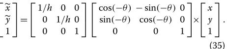
Apart from energy functionals for tracking, the second pertinent issue in object tracking is consideration of possible rotation or scale changes of the object being tracked. Evolution using the above-mentioned function-als may become erroneous for large differences in scale and rotation between the candidate and target level set functionals. To remove this error, the candidate contour is normalised with respect to its rotation and scale with respect to the target before evaluating the tracking energy. Assuming an arbitrary scale parameter h and rotation parameter θ that produces the candidate function c, both the current image frameIand the candidate function care transformed according to:
c(x,y)=c(x,y) (33)
I(x,y)=I(x,y), (34)
wherexandyare calculated as: ⎡
⎣xy 1
⎤ ⎦=
⎡
⎣1/h0 10 0/h 0
0 0 1
⎤ ⎦
⎡
⎣cossin((−−θ )θ ) −cossin(−(−θ )θ ) 00
0 0 1
⎤ ⎦×
⎡ ⎣xy
1 ⎤ ⎦.
(35)
image remain intact: their transformed values are used exclusively for evaluating energy functionals.
5 Experimental results and discussion
The system was implemented in MATLAB and tested using a set of ten maritime sequences obtained from the Council of Science and Industrial Research (South Africa). These sequences include a variety of scenes, weather con-ditions and maritime objects of interest. A specific target object was chosen for each of the sequences and used to test both object detection and tracking—the target objects for each of the sequences. This section introduces per-formance metrics regarding object detection and tracking and uses these metrics to compare the various choices for detection and tracking described previously. Thereafter, the final system is proposed.
5.1 Performance metrics 5.1.1 Object detection
The object detection algorithm is a form of classifica-tion task, where pixels are either classified as belonging to a maritime object or not. The detector’s output is a binary image with pixels that are classified as objects being labelled as 1. Given the actual classification of pixels (ground truth) and the output of the system, four out-comes are possible. Outout-comes where the system agrees with the actual data are labelled true positives (TP) or true negatives (TN) depending on whether the pixel belongs to an object or not. If the system incorrectly labels a pixel as an object when in actuality there is not one there, this is called a false positive (FP), while a false negative (FN) is a case where an object is present but the system fails to detect it. For the classification task,Precisionis defined as, given the actual classifications of particular subjects, the proportion of cases where the subject was classified as positive and was actually the case [37]. In terms of the totals discussed above, Precision is calculated as:
Precision= TP
TP+FP. (36)
Recall is defined as the proportion of subjects which were actually positive and were classified as such [37]. In terms of the above totals:
Recall= TP
TP+FN. (37)
Hripcsak and Rothschild [37] define the F measure, which is a harmonic mean of the two metrics:
Fβ =
(1+β2)×Recall×Precision
β2×Precision+Recall , (38)
whereβis a parameter that allows one to weight Precision or Recall more heavily.Fβ is the notation used to indi-cate theβused in a particularFscore. Szpak and Tapamo [4] note that for a surveillance system, the reduction of
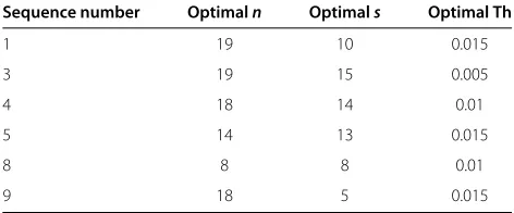
Table 2 Optimal background subtraction parameters for various sequences
Sequence number Optimaln Optimals Optimal Th
1 19 10 0.015
3 19 15 0.005
4 18 14 0.01
5 14 13 0.015
8 8 8 0.01
9 18 5 0.015
false negatives is top priority. For this reason, Recall was weighted twice as much as Precision by settingβ=2. This F score can be used to test both the output of the back-ground subtraction algorithm and the post-filter. To test the accuracy of level set filtering, the output of the post-filtering stage was segmented using binary level set shape prior segmentation for each sequence. For an input binary image withnblobs and assuming that energy is positive at all times, the segmentation proficiency score is defined as:
P= argmini=t≤nE(i)
E(t) , (39)
whereE(x)is the final energy obtained from the level set segmentation of blob x in the image and t is the index of the blob belonging to the object that is to be found. This essentially measures the contrast between the energy associated with segmentation of the actual object and the blob with the lowest energy of the remaining blobs. If the desired object has the lowest energy,Pwill be greater than 1, indicating a correct classification. However, if another blob has a lower energy than the desired object,Pwill be less than 1.
If the object is successfully detected, the quality of its segmentation is measured. Krishnaveni and Radha [38] suggest using Dice’s coefficient [39] as a method of perfor-mance evaluation for level set methods:
s= 2(A∩B)
A+B , (40)
Table 3 Area of the smallest ground truth object in each sequence
Sequence Object area
1 458
3 1047
4 696
5 677
8 70
Figure 4Average Dice’s coefficient versus the number of iterations for various energy terms.
where Aand Bare the ground truth and resultant seg-mentation regions, respectively, ands varies from 0 to 1 depending on the proportion of pixels shared between the ground truth and the segmenting contour.
5.1.2 Object tracking
The tracker detection rate (TDR) is the average number of frames where an object is successfully tracked and is defined by Porikli and Bashir [13] as:
TDR= TPF
TG, (41)
where TPF is the number of frames where the system con-tour overlaps the ground truth object. TG is the number of frames in which the ground truth object is present. There are different strategies to test if object overlap occurs, the simplest of which is to test if the system contour’s cen-troid lies within the ground truth object’s bounding box.
To measure the degree of success for a tracked object, the object tracking error (OTE) [13] is defined as:
OTE= 1
TPF TG
i=1
Dist(pGTi ,pSysi )×G(GTi, Sysi), (42)
where Dist() measures the distance between the centroids for the ground truth objectpGTi and system contourpSysi in the ith frame, respectively. G(GT,Sys) is an overlap function defined as:
G(GT,Sys)=
1 if GT and Sys overlap
0 otherwise. (43)
5.2 Optimisation
There are a number of parameters that need to be decided upon in the object detection and tracking subunits. Given the performance metrics defined in the previous section, the parameter values are deduced in an optimal way.
5.2.1 Object detection
While the common strategy of splitting a dataset into two-thirds for training and one-third for testing is shown to work well for reasonably sized datasets (over 100 cases [40]), this was used for the system dataset despite its small size. The training could be repeated over a larger data set as future work, and the concepts are emphasised here with the term ‘optimal’ being used loosely. Sequences 1, 3, 4, 5, 8 and 9 were randomly chosen as a training set for optimisation, while the remaining sequences were used for testing.
Discussion of the two possible pre-filters, the 3×3 Gaus-sian filter and the 3×3 Median filter, is postponed until last. No optimisation can be performed at the moment, but later in this paper, performance of the two filters is compared.
Figure 6Comparison of variousF2scores for various filtering algorithms.
• Background subtraction. In order to achieve a more satisfactory result, the background subtraction algorithm must be optimised with respect to the following:
– The number of frames used for kernel density estimation (n)
– The spacing between each frame (s) – The probability threshold used (Th)
These variables were adjusted to maximise theF2 score calculated for a small window around an object of interest in an image. A brute force search was run to find optimal parameters for each of the
above-mentioned training sequences. For every sequence, the values ofn,sand Th were varied and the cost function was measured. Those that resulted in the lowest cost function were considered optimal for each sequence and are shown in Table 2. The averages of these parameters were used in the final algorithm hoping that these would give fairly decent results across most of the sequences.
Therefore, the optimally chosen parameters are as follows:
n=16,s=11andTh=0.0117
• Post-filtering. Out of the possible post-filters listed, the fixed threshold connected component algorithm has an optimal threshold based on blob size, while the variable threshold algorithm has an optimal threshold function that may be used. To find an optimal fixed threshold for fixed threshold connected component filtering, the area of the smallest ground truth object in each sequence was measured in order. The algorithm has to filter out blobs which are superfluous but still keep those that belong to actual maritime objects. To do this, a lower threshold for blob size must be selected. Table 3 shows the area of the smallest ground truth object in each sequence. The smallest object, observed in sequence 8, has an area of 70 pixels. To ensure that objects above this size are kept, and allowing 10 pixels for safety, the threshold was set at 60. The area of each of the
training objects was plotted versus its normalised vertical position. The following area threshold function that included each object was chosen:
M(y)=90y+10, (44)
wherey is the normalised vertical position. This function ensures that blobs near the top of the image need only be over 10 pixels in size to be kept in the image, while blobs at the bottom of the image need to have an area over 100 pixels to be kept.
5.2.2 Object tracking
For each possible formulation of the energy functional, the tracking algorithm was run on a hundred frames for various iterations per frame. Three randomly selected sequences were used as a source of these frames. The aver-age Dice’s coefficient versus the number of iterations per frame for each energy term is shown in Figure 4.
5.3 Object detection results
Given the deduced background subtraction and post-filtering parameters, the performance of the object detec-tion subsystems is not measured. The choice of pre-filter is now addressed. The optimised object detection algo-rithm was run on the test set of sequences: sequences 2, 6, 7 and 10. The entire system has been broken into its indi-vidual subsystems which have been tested indiindi-vidually. Subsystems that have a number of different algorithms at their disposal have been tested using each of these techniques and compared.
5.3.1 Background subtraction and pre-filter
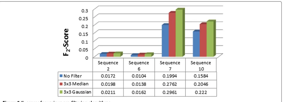
Figure 5 shows F2 scores for various pre-filtering algo-rithms that have been tested. The comparatively low scores for sequences 2 and 6 can be explained by the large amount of glint in sequence 2 and the small object size in sequence 6. Despite these low scores, pre-filtering was able to improve scores for every sequence. It is clear that using the 3×3 Gaussian filter provides the best results, and so this was used for testing in the next stages of the algorithm.
5.3.2 Post-filtering
Figure 6 shows the F2 scores of various post-filtering methods. These have been applied to the output of the
Table 4Pscores for various image sequences using Chan-Vese energy as classification criteria
Sequence Pscore Classification (pass/fail)
2 6.9316 Pass
6 0.4642 Fail
7 4.2569 Pass
10 13.1468 Pass
Table 5 Segmentation results from image sequences that passed level set filtering
Sequence Dice’s coefficient
2 0.8698
7 0.6113
20 0.6667
background subtraction used with a Gaussian pre-filter, and soF2scores for the raw background subtracted out-put have been included for comparison. Every filtering method was able to improve the score for every sequence. F2scores for sequences with large objects are less sensitive to false positives as they do not compare much propor-tionally to the number of pixels in the object. The converse is true for smaller objects such as sequence 6 where the largest improvement from filtering is shown.
As they are the most aggressive filtering methods, it comes as no surprise that the connected component fil-ters (both fixed and variable threshold) give the biggest improvement in scores. One should bear in mind the possibility that if a target were too small, these filtering algorithms would remove it from the image, and so there is an associated risk with using them. Due to its increasing threshold at the bottom of the image, the variable thresh-old connected component algorithm was able to remove more false positives than the fixed threshold, producing the highestF scores out of all the filters. This algorithm yielded an average increase of 78% in F2 scores for all
Table 6 Performance metrics for each sequence
Sequence TDR OTE
1 1 1.8795
2 1 3.7144
3 1 1.4506
4 0.85 10.799
5 0.71 4.8505
6 0.38 7.2204
7 1 20.62
8 1 2.7759
9 0.7933 1.5088
10 1 2.6944
The sequences have been calculated using sequences of 300 frames.
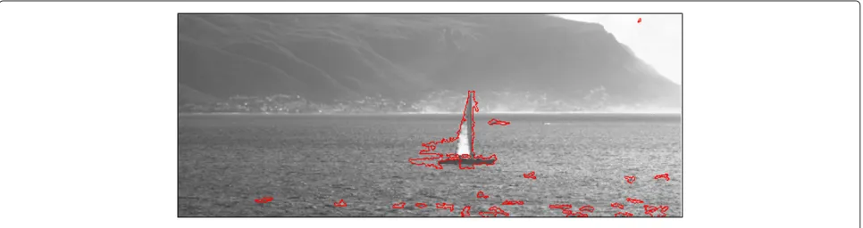
test sequences. The inability of post-filtering algorithms to improve test scores in sequence 2 can be attributed to the large amount of glint and ocean movement in the image. Figure 7 shows the output of post-filtering, where the majority of false positives at the bottom of the image are removed.
5.3.3 Level set filtering
To test the level set segmentation technique, the output from the variable threshold connected component algo-rithm was used as input data as it had the best results out of all the filtering methods. Table 4 showsP scores for each sequence and indicates which passed or failed at clas-sification. Apart from sequence 6, all the sequences were correctly classified with very goodPscores. A likely rea-son for sequence 6’s failure is the similarity in the shape of the blob around the ship with false positive blobs in the image. Despite its poorF2score, the algorithm was able to locate the object in sequence 2. Table 5 shows actual segmentation results for the sequences that were correctly classified.
While sequence 2 can be considered as a good seg-mentation, smudging effects from the background sub-traction algorithm caused poor segmentation results for sequences 7 and 10. These smudging effects trailing the objects are simply artefacts of the threshold selection for
the sequences. As the ship in sequence 10 (Figure 8), for example, moves from right to left, its pixel values become part of the density estimate for pixels trailing it. This decreases the probability of seeing a sea pixel, and so when one is seen, this may be marked as the foreground if the threshold is not set low enough. The segmenting con-tours have tried to position themselves to include as many of these pixels as possible resulting in offsets from the ground truth.
5.4 Object tracking results
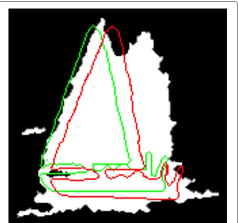
Table 6 shows TDR and OTE for each sequence. The main reason for poor performance in sequences (especially 4 and 5) can be attributed to change in frequency charac-teristics of the pixels that make up target objects. Figure 9 shows an example of this from sequence 5. The target con-tour in the first frame (above, in yellow) and the tracking contour in the frame where it starts to drift away from the object (bottom, in red) are shown. In this case, glint from the sun strongly defines the borders of the object in the target frame, while the contour starts to drift when this glint is no longer present, making the target almost indistinguishable from the background to the human eye. Poor tracking results in sequence 6 can be attributed to small object size and similar frequency characteristics of the object with the ocean, whereas camera panning ruined the otherwise perfect tracking results in sequence 9. Although the tracking contour successfully overlapped the object in every frame of sequence 7, the sequence has a comparatively high object tracking error of 20.62. This is due to a local minimum in the tracking energy functional under the object that left the tracking contour offset from its target in most frames.
5.5 Speed of algorithm
On a 2.0-GHz dual-core processor, our system could process approximately ten frames per second with a MATLAB implementation of the algorithms. This per-formance can be greatly improved by doing a C++ implementation and parallelising some of the algorithms (e.g. background subtraction). The running time of the video tracker developed has purposefully been given
lesser priority in order to focus on the development of concepts and methodology. Since this work addresses unexplored topics, the main focus is on the development of models and algorithms to address fundamental issues rather than address supplementary practical issues such as algorithm speed which may be optimised in future work for real-time computing.
6 Conclusions
This paper has investigated the use of prior knowledge of a ship shape to assist level set segmentation in video tracking for a maritime surveillance problem. It shows that integrating shape priors into level set segmentation is fea-sible and results in promising video tracking performance. While the system did produce an acceptable set of results, it still requires some assumptions that would not be prac-tical in a real-life situation. Future work would allow for relaxation of these assumptions. The system only uses a single shape prior that must be manually preset for every sequence that would not be feasible in a real-life system. To remove the reliance on the user, a bank of multiple training shapes could be modelled using a method such as kernel density estimation. This model would then be used in place of a fixed shape prior for segmentation. It has to be noted that the system would be far more accurate if trained with a larger training set.
Competing interests
Both authors declare that they have no competing interests.
Acknowledgements
The authors gratefully acknowledge PRISM/CSIR for funding this research. We would also like to thank the Optronic Sensor Systems at the Center for Scientific and Industrial Research (CSIR) for making the dataset available.
Received: 14 February 2013 Accepted: 2 July 2013 Published: 26 July 2013
References
1. G Stubblefield, B Parlatore, Condition yellow. PassageMaker, Winter, 85 (1999)
2. Piracy attacks in East and West Africa dominate world report (ICC Commercial Crime Services, 2012), [http://www.icc-ccs.org/news/711-piracy-attacks-in-east-and-west-africa-dominate-world-report]. Accessed 09 Nov 2012
3. J Sanderson, M Teal, T Ellis, Characterisation of a complex maritime scene using Fourier space analysis to identify small craft, inSeventh International Conference on Image Processing and its Applications(Conf. Publ. No. 465), vol. 2 (IEE, Manchester, 1999), pp. 803–807
4. ZL Szapk, JR Tapamo, Maritime surveillance: tracking ships inside a dynamic background using a fast level-set. Expert Syst Appl.38(6), 6668–6680 (2011)
5. PL Herselman, CJ Baker, de HJ Wind, An analysis of X-band calibrated sea clutter and small boat reflectivity at medium-to-low grazing angles. Int. J. Navigation Observation (2008). doi:10.1155/2008/347518
6. R Vicen-Bueno, R Carrasco-Alvarez, M Rosa-Zurera, JC Nieto-Borge, Sea clutter reduction and target enhancement by neural networks in a marine radar system. Sensors.2009(9), 1913–1936 (2009) 7. P Westall, J Ford, P O’Shea, S Hrabar, Evaluation of machine vision
techniques for aerial search of humans in maritime environments, in Digital Image Computing: Techniques and Applications (DICTA) 2008 (Canberra, 1–3 Dec. 2008), pp. 176–183
8. A Maistrou, Level set methods - overview (2008), [http://campar.in.tum. de/twiki/pub/Chair/TeachingSs08EvolvingContoursHauptseminar/ ActiveContours.pdf]
9. M Kass, A Witkin, D Terzopoulos, Snakes: active contour models. Int J. Comput. Vis.1(4), 321–331 (1988)
10. T Chan, LA Vese, Active contours without edges. IEEE Trans Image Proces. 10(2), 266–277 (2001)
11. S Osher, J Sethian, Fronts propagating with curvature-dependent speed: algorithms based on Hamilton-Jacobi formulations J. Comput. Phys.79, 12–49 (1987)
12. D Cremers, Dynamical statistical shape priors for level set based tracking. IEEE Trans. Pattern Anal. Mach. Intell.28(8), 1262–1273 (2006)
13. F Bashir, F Porikli, Performance evaluation of object detection and tracking systems, inIEEE International Workshop on Performance Evaluation of Tracking and Surveillance (PETS)(IEEE Computer Society, New York, 2006), pp. 7–14
14. T Chan, W Zhu, Level set based shape prior segmentation, inIEEE Computer Society Conference on Computer Vision and Pattern Recognition, Volume 2 of CVPR 2005(San Diego, 20–25 June 2005), pp. 1164–1170 15. M Rousson, N Paragios, Shape priors for level set representations, in
Computer Vision – ECCV 2002, ed. by A Heyden, G Sparr, M Nielsen, and P Johansen,Lecture Notes in Computer Science, vol. 2351 (Springer, 1039 Heidelberg, 2002), pp. 78–92
16. AJ Tsai, A Yezzi, W Wells, D Tempany, C Tucker, A Fan, W Grimson, A Willsky, shape-based approach to the segmentation of medical imagery using level sets. IEEE Trans. Med. Imaging.22(2), 137–154 (2003) 17. M Rousson, N Paragios, R Deriche, Implicit active shape models for 3D
segmentation in MRI imaging, inMedical Image Computing and Computer Assisted Intervention – MICCAI 2004, ed. by C Barrillot, DR Haynor, and P Hellier (Springer, Heidelberg, 2004), pp. 209–216
18. D Cremers, S Osher, S Soatto, Kernel density estimation intrinsic alignment for shape priors in level set segmentation. Int. J. Comput. Vis. 60(3), 335–351 (2006)
19. AA Smith, M Teal, Identification and tracking of maritime objects in near-infrared image sequences for collision avoidance, inSeventh International Conference on Image Processing and its Applications(Conf. Publ. No. 465), vol. 1 (IEE, Manchester, 1999), pp. 250–254
20. P Voles, M Teal, Maritime scene segmentation, http://homepages.inf.ed. ac.uk/rbf/CVonline/LOCAL_COPIES/VOLES/marine.html. Accessed 12/04/2012
21. P Voles, M Teal, J Sanderson, Target identification in a complex maritime scene, inIEE Colloquium on Motion Analysis and Tracking(IEE, London, 1999), pp. 15/1–15/4
22. KM Gupta, DW Aha, R Hartley, PG Moore, Adaptive maritime video surveillance, inProceedings of SPIE-09, Volume 7346 of Visual Analytics for Homeland Defense and Security(SPIE, Bellingham, 2009)
23. AM Ponsford, L Sevgi, H Chan, An integrated maritime surveillance system based on high-frequency surface-wave radars. 2. Operational status and system performance. IEEE Antennas Propagation Mag.43(5), 52–63 (2001)
24. H Leung, N Dubash, N Xie, Detection of small objects in clutter using a GA-RBF neural network. IEEE Trans. Aerosp. Electron. Syst.38, 98–118 (2002)
25. R Vicen-Bueno, R Carrasco-Alvarez, M Rosa-Zurera, J Nieto-Borge, M Jarabo-Amores, Artificial neural network-based clutter reduction systems for ship size estimation in maritime radars. EURASIP J. Adv. Signal Process. 2010(9), 380473 (2010)
26. D Socek, D Culibrk, O Marques, H Kalva, B Furht, A hybrid color-based foreground object detection method for automated marine surveillance, inAdvanced Concepts for Intelligent Vision Systems – ACIVS 2005,ed. by J Blanc-Talon, W Philips, D Popescu, and P Scheunders, Lecture Notes in Computer Science, vol. 3708 (Springer, Heidelberg, 2005), pp. 340–347 27. S Fefilatyev, D Goldgof, C Lembke, Tracking ships from fast moving camera
through image registration, in2010 International Conference on Pattern Recognition(IEEE Computer Society, Los Alamitos, 2010), pp. 3500–3503 28. M Michael Seibert, BJ Rhodes, NA Bomberger, PO Beane, JJ Sroka, W
29. M Bertalmio, G Sapiro, G Randall, Morphing active contours. IEEE Trans. Pattern Anal. Mach. Int.22(7), 733–737 (2000)
30. A Yilmaz, O Javed, M Shah, Object tracking: a survey. Surv.38(4), 13–20 (2006)
31. C Bibby, I Reid, Real-time tracking of multiple occluding objects using level sets, inProceedings of the IEEE Conference on Computer Vision and Pattern Recognition(IEEE, Los Alamitos, 2010), pp. 1307–1314
32. Y Shi, W Karl, Real-time tracking using level sets, inProceedings of the IEEE Conference on Computer Vision and Pattern Recognition, vol. 2 (IEEE, Los Alamitos, 2005), pp. 34–41
33. A Elgammal, R Duraiswami, Background and foreground modeling using nonparametric kernel density estimation for visual surveillance. Proc. IEEE. 90, 1151–1163 (2002)
34. B Silverman, Density estimation for statistics and data analysis. Monogr. Stat. Appl. Probability.1, 1–22 (1986)
35. A Harvey, V Oryshchenko, Kernel density estimation for time series data. Int. J. Forecasting.28, 3–14 (2012)
36. A Yezzi, A Tsai, A Willsky, A statistical approach to snakes for bimodal and trimodal imagery, inProceedings of the Seventh IEEE International Conference on Computer Vision, Volume 2 of ICCV 1999(Kerkyra, 20–27 Sept 1999), pp. 898–903
37. G Hripcsak, A Rothschild, Agreement, the F-measure, and reliability in information retrieval. J. Am. Med. Inf. Assoc.12(3), 296–298 (2005) 38. M Krishnaveni, V Radha, Quantitative evaluation of segmentation
algorithms based on level set method for ISL datasets. Int. J. Comput. Sci. Eng.3(2), 2361–2369 (2011)
39. L Dice, Measures of the amount of ecologic association between species. Ecology.26(3), 297–302 (1945)
40. K Dobbin, R Simon, Optimally splitting cases for training and testing high dimensional classifiers. BMC Med. Genomics.41(7), 1–31 (2011)
doi:10.1186/1687-5281-2013-42
Cite this article as:Frost and Tapamo:Detection and tracking of
mov-ing objects in a maritime environment usmov-ing level set with shape priors. EURASIP Journal on Image and Video Processing20132013:42.
Submit your manuscript to a
journal and benefi t from:
7Convenient online submission 7Rigorous peer review
7Immediate publication on acceptance 7Open access: articles freely available online 7High visibility within the fi eld
7Retaining the copyright to your article