ACKMOWI.ED6E1IE1ITS
Financial support for this work came from WRRI/US
Geological Survey Grant Number 89-0496. Ciba Geigy
Corporation provided the herbicides. Thanks for technical
ELIZABETH M. NELSON. An investigation into the Effects of Heterogeneity on Subsurface Flow and Transport. (under the direction of Cass T. Miller)
ABSTRACT
The risk of groundwater contamination by land-applied organic chemicals is a growing concern. Prediction of the
fate and persistence of contaminants in the subsurface is desircUsle. Soil hydraulic properties are rarely homogeneous and their transient nature has a profound effect on fluid
flow and solute transport. Evidence suggests that sorption
is a significant process impacting the movement of contaminants through the unsaturated zone.
Sorption rate and equilibrium experiments were conducted in completely mixed batch reactors using
metolachlor on two soil columns divided into 12 segments each. The equilibrium data were modeled with the linear
model and the Freundlich expression. A surface-diffusion
model was used to describe the rate data. The results of
these laboratory studies were used in conjunction with field
data acquired using soil columns in the vicinity of the site
from whence the laboratory soils came to test the Pesticide
Root Zone Model (PRZM).
The results of these experiments showed that the
equilibrium data were nonlinear and best fit with the
Freundlich expression. However, the linear partition coefficients were highly correlated with the fraction of
TABI.E OF COMTEMTS
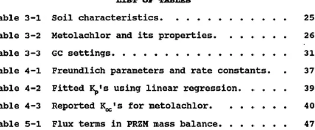
LIST OP FIGURES... vi
LIST OP TABLES... vii
LIST OF SYMBOLS... viii
I INTRODUCTION ... 1
1.1 Background... 1
1.2 Objectives... 4
II THEORY... 5
2.1 Flow and Transport in the Unsaturated Zone . 5
2.1.1 Flow... 62.1.1.1 Hysteresis ... 7
2.1.2 Transport... 11
2.1.2.1 Sorption ... 12
2.1.2.1.1 Sorption Equilibrium Theory... 12
2.1.2.1.2 Sorption Rate Theory . . 16
2.2 Unsaturated Zone Modeling... 19
2.2.1 Research Models... 20
2.2.2 Management Models ... 23
III EXPERIMENTAL METHODS ... 24
3.1 Materials... 24
3.2 Total Organic Carbon Analysis ... 27
3.3 Sorption Rate Studies... 28
3.4 Sorption Equilibrium Studies ... 29
3.5 Analytical Methods ... 30
IV EXPERIMENTAL RESULTS AND DISCUSSION ... 32
4.1 Introduction ... 32
4.2 Organic Carbon Analysis ... 32
4.3 Sorption Rate Studies... 33
4.4 Sorption Equilibrium Studies ... 36
4.5 Modeling of Experimental Data... 41
V MODELING OF FIELD DATA... 46
5.1 Introduction ... 46
5.2 Mass Balance... 46
5.2.1 Transport Parameter Input ... 49
5.3 Water Balance... 51
5.3.1 Water Balance Parameter Input ... 54
5.4 Input Files... 55
5.5 Model Results... 56
VI CONCLUSIONS AND RECOMMENDATIONS ... 65
6.2 Recommendations... 66
LIST 07 FIGDBES
Figure 2-1 Hypothetical soil moisture hysteresis
curves... 8 Figure 4-1 %TOC as a function of column and depth. . . 33 Figure 4-2 Metolachlor kinetic data. Mil column. ... 35 Figure 4-3 Metolachlor kinetic data, Mil 82.5-90. . . 35
Figure 4-4 Metolachlor equilibrium data and Freundlich
fits... 38
Figure 4-5 R v. %TOC for metolachlor on 24 soils. . . 40 Figure 4-6 Diffusion rate model fit, M18 33-36. ... 42 Figure 4-7 Diffusion rate model fit. Mil 9-12... 42 Figure 4-8 Diffusion rate model fit. Mil 37.5-45. . . 42
Figure 5-1 PRZM flow calibration for WITH PLANT. ... 56
Figure 5-2 PRZM flow calibration for NO PLANT... 57 Figure 5-3 Experimental (Keller, 1991) and
PRZM-predicted tritium concentration at end
of 1 month... 59
Figure 5-4 Experimental (Keller, 1991) and PRZM-predicted tritium concentration at end
of 2 months... 59 Figure 5-5 Field data (Keller, 1991) v. PRZM data at
end of 1 month... 60 Figure 5-6 Field data (Keller, 1991) v. PRZM data at
end of 3 months... 61 Figure 5-7 Field data (Keller, 1991) v. PRZM data at
I.IST OI* TABLES
Table 3-1 Soil characteristics... 25
Table 3-2 Metolachlor and its properties... 26
Table 3-3 GC settings... 31
Table 4-1 Freundlich parameters and rate constants. . 37
Table 4-2 Fitted K 's using linear regression... 39
LIST OF SYMBOLS
A cross-sectional area of the soil column (L^)
\ watershed area (L^)
c specific moisture capacity (l}/l?)
C fluid-phase concentration (M/L^)
Cg fluid-phase concentration at equilibrium with
solid-phase solute concentration at exterior of solid
particle (M/L^)
Cg^ sorbed-phase concentration in PRZM equations (M/M)
C^ fluid-phase concentration in PRZM equations (M/Lj)
D hydrodynamic dispersion coefficient (lVt)
Dg surface-diffusion coefficient (l^/T)
E extraction coefficient (L'^)
Ey evaporation (L/T)
f fraction of total water in zone used for evaporation
foe fraction of organic carbon (M/M)
F fraction of the application intercepted by the plant
hA reversal pressure head for scanning curves (L)
I percolation (L/T)
Jp flux due to dispersion (M/T)
J^ flux due to advection (M/T)
Jpy flux due to transformation of the fluid-phase (M/T)
J^j flux due to plant uptake of fluid-phase (M/T)
Jqj. flux due to removal in runoff (M/T)
J^pp flux due to pesticide application (M/T)
jpQP flux due to washoff from plants to soil (M/T)
J„ flux due to transformation of sorbed-phase (M/T)
Jgu flux due to removal on eroded recliments (M/T)
J^g flux due to adsorption (M/T)
Jpgg flux due to desorptionn (M/T)
k^ external film mass-transfer coefficient (L/T)
kg lumped first-order degradation rate for PRZM (L/T)
Kf Freundlich sorption capacity constant ([lVm]")
K^ carbon-normalized linear partition coefficient (lVm)
K^ octanol-water partition coefficient
Kp linear partition coefficient (lVm)
Kj hydraulic conductivity in the vertical direction (L/T)
m,n hysteresis curve shape parameters
M mass of sorbent in reactor
M mass of pesticide on plant surface per area (M/L^)
n^ Freundlich exponent
P precipitation as rainfall minus crop interception (L/T)
P^ daily rainfall depth (LL/T)
q water flux density (L/T)
Q solid-phase concentration (M/M)
Q average concentration in one particle (M/M)
Q^ solid-phase concentration as a function of radial
position (M/M)
Q|.y daily runoff depth (L/T)
r radial position in spherical particle (L)
r enrichment ratio for organic matter (M/M)
onR solid particle radius (L)
S effective saturation
e
t time (T)
U transpiration (L/T)
V pore velocity (L/T)
V volume of solution in reactor (L')
AX depth of compartment for PRZM (L)
Xg erosion sediment loss (M/T)
z vertical distance (L)
a hysteresis curve shape parameter
e dimensionless uptake efficiency factor
t pressure head in unsaturated zone (L)
0 source or sink term (M/L^T)
p soil bulk density (M/L^)
0 volumetric water content {J?/I?)
0^ residual moisture content (lVl')
I IMTBODUCTIOH
1.1 Background
The use of land-applied organic chemicals in the form
of pesticides, herbicides and fungicides is widespread in
the United States. Normal use as well as misuse has
resulted in detection of more than 70 pesticides in
groundwater sources in 38 states (Ritter, 1990). The
toxicity of such groundwater contaminants has raised public
concern and motivated research directed towards predicting
the fate and persistence of surface-applied organic
chemicals in the subsurface. The risk of groundwater
contamination from agricultural pesticide use is ultimately
determined by the relative rates of percolation and
degradation within the vadose zone and by the factors that
control them (Bowman, 1988).Following Brady (1990), the vadose zone of the
subsurface is that region of the subsurface environment
extending from the ground surface through the root zone to
the saturated zone interface. It is a complex ecosystem in
which the soil is profiled into more or less distinct
synthetic organic chemicals. The uppermost layers are more
weathered than the lower layers, while the lower layers
often contain the weathering products such as organic acids,
silicate clays and hydrous oxides of iron and aluminum
oxides which have leached from the upper layers.
Heterogeneous soil properties resulting from this layering
include pH, clay content, organic content, soil texture and
bulk density. As mentioned, these soil properties have an
effect on solute transport, and their heterogeneous nature
in the soil profile complicates the prediction of pesticide
persistence.
In order to understand vertical movement of
contaminants through the unsaturated soil zone, the
distinction must be made between transport of the organic
chemical and flow of the water. Vertical water flow in the
vadose zone is governed by soil hydraulic properties such as
the relationships between hydraulic conductivity, volumetric
water content and pressure head. Soil layering in the
unsaturated zone results in spatial variability of hydraulic
properties and has been found to be significant. Russo and
Bresler (1981) report that soil hydraulic properties may
vary substantially over short distances in the vertical
direction. Modeling unsaturated flow requires
characterization of soil hydraulic properties for
Contaminant transport through porous media is affected by several mechanisms. These mechanisms include
hydrodynamic transport, uptake of solute by plants, runoff
or volatilization at the surface and sorption to the solid
matrix (Weber and Miller, 1989). The magnitude of each of
these processes must be understood to determine a
pesticide's tendency to migrate into the saturated zone
where it would pose a groundwater contamination threat. In
addition, the solute may be transformed by chemical
processes such as hydrolysis or photodecomposition or
biochemical modification by soil organisms. The persistence
of a solute in the soil depends on all of the transport and
degradation processes affecting it.
Sorption of the solute to the soil matrix has been found to be an important mechanism determining the
persistence of contaminants in the soil. The effect of
pesticide sorption on a soil is to reduce the concentration
in solution thereby retarding pesticide movement through the
root zone. The extent of the retardation is chemical and
soil specific, and depends on such factors as solute
hydrophobicity and volatility, and soil pH, organic content
and clay content. It is, therefore, important to know the
site-specific chemical and soil properties if one is to
predict solute sorption phenomena in the field.
The complexity of agroecosystems requires a model that
unsaturated flow phenomenon to predict the fate and
transport of pesticides. The data required for such models requires both field and laboratory studies to characterize the range of physical, chemical and biological influences in the ecosystem. Models and data such as these provide
knowledge relevant to the mobility, dissipation and potential for groundwater pollution by soil applied
toxicants.
1.2 Objectives
The overall objective of this work was to determine the effect of spatial variability on solute transport in the
unsaturated zone. The subobjectives of this work were: to
determine variations in sorptive characteristics at a fine scale, to investigate correlations in the structure of the
II THEORY
Prediction of surface applied pesticide fate and
transport is desirable given the potential environmental
impact of trace organics in groundwater. Such prediction
requires an understanding of what happens to the pesticide
once it is applied. The transient processes affecting
pesticide fate include water flow, plant extraction,
degradation and sorption. The complexity of such
interactions between pesticides and soil material have led
to the development of a variety of approaches to estimate
pesticide fate and persistence in the vadose zone. The
differences in approach are distinguished by the way in
which the developer accounts for the transient processes
mentioned above. In this chapter, unsaturated zone flow and
transport phenomena and their transient nature are
discussed. Since the focus of this work was on sorption
processes in the unsaturated zone, sorption theory is
presented in some detail. The final topic of this chapter
deals with unsaturated zone modeling theory and the
advantages and shortcomings of various models.
2.1 Flow and Transport in the Unsaturated Zone
accounted for separately to accurately predict contaminant
movement. The intricacies of modeling these phenomena are
presented below.
2.1.1 Flow
Vertical water flow through the unsaturated zone can be
mathematically described using Richards' equation which is
derived from Darcy's law and the continuity equation
where f is the pressure head in the unsaturated zone, and K^
is the hydraulic conductivity in the vertical direction, z.
This equation is highly nonlinear by virtue of the transient
nature of hydraulic conductivity, volumetric water content
and pressure head. The specific moisture capacity, c, is
given by
c(t) - -* 2.2
where 6 is the volumetric water content. Equation 2.1 is
very definitely nonlinear especially when the hysteretic
nature of the specific moisture capacity (c) is considered.
Numerical solutions have been presented by Freeze (1971) and
2.1.1.1 Hysteresis
Periodic changes in irrigation flux or evaporation rate cause the soil water content to undergo wetting and drying cycles (Russo et al., 1989a). The equilibrium soil water
content at a given suction pressure is greater in the drying
cycle than the wetting cycle. This hysteresis effect during
such wetting and drying cycles has been studied extensively (Poulovassilis, 1970; Mualem, 1974; 1976; van Genuchten, 1980; Luckner, et al., 1989). Soil property hysteresis may
be attributed to several causes (Hillel, 1971): the
geometric nonuniformity of individual pores causing
variations in capillary wetting and draining, the contact
angle of water on the pore walls causing an advancing meniscus to have a greater radius of curvature than a
receding one, entrapped air decreasing the water content of newly wetted soil, and swelling and shrinking phenomena
resulting in differential changes of soil structure
depending on the wetting and drying history of the soil. While incorporating hysteretic effects into the flow model
(Equation 2.1) is complex and requires additional
computational effort, Russo et al. (1989a) suggested that
neglecting hysteresis under nonmonotonic transient flow
conditions may lead to underestimating solute travel time
through the surface zone because calculated water contents
are higher near the surface when hysteresis is included.
model. A hypothetical hysteresis curve is found in Figure
2-1.
0.00 0.10 0.20 0.30
Theta (cm + *3/cm**3)
0.40
Figure 2-1 Hypothetical soil moisture hysteresis curves.
Models to describe soil property hysteresis have been both empirical and theoretically based. As discussed by Kool and Parker (1987), empirical models have been used to describe hysteresis in specific soils or porous media, while
theoretical models based on the domain theory of capillary
hysteresis (Topp, 1971; Mualem, 1974) have more universal
validity. In the model defined by Kool and Parker (1987),
the main wetting and drying retention curves characterize
the hysteretic relationship between pressure head and volumetric water content as soil moisture content changes
from its residual moisture content, 6^, to its saturated
moisture content, 9^, and back. The relationship was
6 — fl
ͣ
^8- -5—^ - [l+\(tH"]-'" h<0 2.3
where S^ is the effective saturation, a and n are curve
shape parameters and m=l-l/n. The main hysteresis loop may
be described by the parameter vectors (6s"/6p"/a",n") and
(6g*^,6p'*,a'',n*^) where the superscripts w and d stand for
wetting and drying respectively (Kool and Parker, 1987).
This gives a total of eight unknown parameters. The main
hysteresis curve is often simplified by assuming it is
closed at the saturated and residual endpoints i.e. 6^" = 6^''
= 6g and 6^" = e^** = 6^. Mualem (1974), however, pointed out
that air entrapment in the soil would cause 6^*^ # 6^", thus
these parameters should be accounted for individually for
increased model accuracy. The unknown curve parameters may
be obtained by using a nonlinear curve fitting procedure to
fit Equation 2.3 to experimentally determined values of 8
and f.
Scanning curves describe the hysteresis effect between
the residual and saturated limits of the main wetting and
drying curves. Primary scanning curves are those that
depart directly from the main curves, while secondary
scanning curves depart from primary curves (Jaynes, 1984).
Kool and Parker, (1987) use an empirical model to describe
e.-e.[i-^/(hj3
Sfihj
e-e.,5/(Aj
e*^ - -A ^s^e v"^/ 2.5
6g* defines the drying scanning curve and 0^* the wetting
scanning curve. Sg*^(h^) is the value of the effective
saturation on the main drying curve at the reversal pressure
head (h^) and S^^Ch^) is the corresponding value on the main
wetting curve. 9^ and 6^ are the water contents at the
reversal points.
van Genuchten (1980) gave the following expression for
hydraulic conductivity
jco) - jc^e'^ri-d-ei/") "i^ 2.6
where K^ is the saturated conductivity. Kool and Parker
(1987) reported that K(e) predicted from Equation 2.6
compares favorably with experimentally obtained values.
They further reported that K(6) of soils generally exhibits
little hysteresis.
The preceding paragraphs indicate the complexity of
soil hydraulic property hysteresis and the number of
parameters it can introduce to a model. In their evaluation
of closed form expressions for hysteretic soil properties,
Equations 2.3 through 2.6 to 8 field soils. They tested
various model simplifications such as letting n^^ = n^^ and 0^*^
= 6^", and concluded that the simplifications would not lead
to an unacceptable loss in accuracy for media with fairly wide pore size distributions. A desired feature of the Kool and Parker model is that the required experimental input is only the main wetting and drying curves and the saturated hydraulic conductivity, also called p-S-K relationships.2.1.2 Transport
The transport of a solute in the vertical direction
through porous media has been well documented and is
described in one dimension by the advective-dispersive-reactive equation
3(60
a [eD(e,g)-|g] - li^-(ll£^)„ . <i>(z,t)
dC dz" " '^' dz' dz " dt '^^^
2.7
where C is the solute concentration, Q is the solid phase solute concentration, D is the hydrodynamic dispersion
coefficient, q is the water flux density, 6 is the
volumetric water content, p is the soil bulk density, 0 is a
source or sink term and z and t are distance and time
respectively. The solute transport equation includes
indicates the dependency of hydrodynamic dispersion on
volvimetric water content and water flux density.
2.1.2.1 Sorption
The transport equation (Equation 2.7) includes a term to account for sorption, a fate mechanism involving the mass
transfer to and from the solid phase. Sorption is a retention process in which there is an accumulation of
solute at the soil-water or soil-air interface. It is a
general term which makes no distinction between the specific
processes of absorption, adsorption and precipitation.
Sorption, studied extensively in recent years, is a highly complex process made so by the high degree of variability in
sorbate/sorbent composition, chemical nature of the sorbate,
and various sorptive interactions occurring in the subsurface. It follows then, that pesticide sorptive
behavior is affected by both soil and solute characteristics (Karickhoff, 1984). Quantitative sorption description
requires a definition of the equilibrium relationships
ultimately attained and the rate at which such relationships
are approached.
2.1.2.1.1 Sorption Equilibrium Theory
Sorption of hydrophobic nonpolar compounds is a
sorption may be assumed to be characterized by linear,
reversible and singular isotherms (Brusseau and Rao, 1989a). The equilibrium relationship for this assumption takes the form of
Qe-KpC^ 2.8
where Q^ is the equilibrium solid-phase concentration, C^ is
the equilibrium fluid-phase concentration and \ is the
linear sorption coefficient. Hydrophobic partitioning has been well documented in the literature (Chiou et al., 1983; Karickhoff, 1984) and it has been found that sorption of hydrophobic organic compounds in soils is more highly correlated to the soil organic carbon content than other soil properties such as clay mineral content and cation exchange capacity (Schwarzenbach and Westall, 1981;
Karickhoff, 1981; 1984; Voice and Weber, 1985). As such,
the linear partition coefficient is often normalized by the
fraction of organic carbon, f^, of the soil.
Koc-^ 2.9
K^ is the organic carbon referenced sorption partition
coefficient and has been found to be largely, but not
or geographic origin (Karickhoff, 1984). Variations in K^
between different solid materials may result from other soil
properties (clay content, cation exchange capacity, pH,
surface area), variations in the nature of the organic
matter present and differences in experimental procedure
(Gerstl, 1990). The relative invariance of K^ allows the
estimation of ¥L for a given solute-sorbent system whose f^^
is known.
The importance of K^ in predicting soil sorption
characteristics has led to development of correlations to
predict K^ from other chemical properties such as log
octanol-water partition coefficient (Schwarzenbach and
Westall, 1981; Karickhoff et al., 1979). Researchers
proposed a linear regression of the form
LogK^^ - ALogK^„ + B 2 .10
where A and B are data fitted coefficients and K„„ is the
octanol-water partition coefficient (Schwarzenbach and
Westall, 1981; Karickhoff et al., 1979; Karickhoff, 1984).
The assumption of linear equilibrium distribution
relationships is generally only applicable to relatively
dilute aqueous systems (Chiou et al., 1979; Karickhoff,
1984). A definite nonlinear relationship, or
concentration-dependent partitioning between fluid- and solid-phase, is
often evident when a broad range of initial fluid-phase
experiments (Weber and Miller, 1989). Nonlinear relationships also occur when mechanisms other than hydrophobic partitioning take place (Brusseau and Rao,
1989a). Highly polar solutes and ionic solutes, for which
site-specific sorption mechanisms are important, often
exhibit nonlinear equilibrixun distribution relationships, and sorption favorability decreases as solute concentration increases as the site-specific mechanisms are influenced by sorbent surface-limited effects (Brusseau and Rao, 1989b).
The nonlinear equilibrium distribution relationship is
often represented by the Freundlich equation
K,CV
2.11where K^ and n^ are empirical constants relating to
sorption capacity and to sorption intensity respectively. The constants may be determined by fitting experimental data
to the linear relationship
LogQ^ - LogKf + iifLogC^ 2.12
While equilibrium data may often be best fit to the
Freundlich model, the linear equilibrium model is obviously
more easily incorporated into the transport equation with
losses in accuracy being a function of the degree of
2.1.2.1.2 Sorption Rate Theory
The rate of solute uptake for a nondegrading solute in a continuously mixed batch reactor (CMBR) is given by
dC M do , T^
dt V dt
where M is the mass of sorbent in the reactor and V is the
volume of solution in the reactor. The dQ/dt term is
defined by an appropriate rate model. The rate of approach
to sorption equilibrium has been studied extensively and, in
general, experimental results show that the sorption process is rate controlled exhibiting two-stage behavior: an
initial short rapid rate of uptake followed by an extended
period of slower uptake (Miller and Weber, 1986; Wu and
Gschwend, 1986; Brusseau and Rao, 1989b).
Two general forms of nonequilibrium, chemical or
physical, are used to describe sorption kinetics. The form
of nonequilibrium is dependent on the mechanism responsible for the nonequilibrium (Brusseau and Rao, 1989b). Physical diffusion models have been shown to characterize sorption kinetic data fairly well (Goltz and Roberts, 1986; Miller and Weber, 1986; Wu and Gschwend, 1986). Ongoing debate exists as to the relative dominance of mass transport into
the solid particle by surface diffusion, pore diffusion or
intraorganic matter diffusion (Brusseau and Rao, 1989a,
1991). Crittenden et al. (1986) suggested that using either a pore diffusion or surface diffusion model would produce the same results for isotherm nonlinearity > 0.8. Brusseau and Rao (1989a) reasoned and showed strong indirect evidence that, for hydrophobic organic compounds, intraorganic matter
diffusion was the likely mechanism causing sorption
nonequilibrixim.
Physical diffusion models consider the rate of sorption to be controlled by a series of mass transfer steps:
diffusion through the bulk fluid (in the mobile region), diffusion across the adsorbed water and diffusion within the
particle itself (in an immobile region). The mobile phase is considered to be well mixed and its resistance negligible
(Brusseau and Rao, 1989b). Further, if the system is
significantly agitated (as is the case for tumbled continuously mixed batch reactors), the diffusion rate
across the boundary film is significantly fast such that the
rate limiting step in the sorption process is diffusive
transport within the immobile region (Weber and Miller,
1988). The sorption reaction itself is assumed to be instantaneous (Brusseau and Rao, 1989b).
A surface-diffusion approach, modeling the process by
Fickian diffusion, was presented by Miller and Weber (1986). The model describes sorption by a mass transfer process
through a boundary layer surrounding a solid particle
dual-resistance model is described in Equations 2.14 through 2.17. For spherical geometry the generalized form of Pick's
Second Law is
where Q^. is the solid-phase concentration as a function of
radial position, r, and D^ the intraparticle effective
diffusion coefficient. The boundary and initial conditions
for Equation 2.8 are (Pedit and Miller, 1988)
dr
\(C-C.) 2.15
Z-R Ds9
BQr
dz - 0 2.16
r-O
Or {O^I^R, t-0) - 0 2.17
where k^ is the external film mass transfer coefficient and
Cg is the fluid-phase concentration at equilibrium with
solid-phase solute concentrations at the exterior of the
particle and R is the solid particle radius. Equation 2.15 sets the flux into the particle equal to the flux out of the
the appropriate equilibrium relationship. A nonlinear
equilibrium relationship would necessitate a numerical
solution to the model (Pedit and Miller, 1988). The average concentration in one particle, Q, is equal to the
integration of Q(r) over the whole sphere.
Q--— f^r^Qir) dz 2.18
P3 Jo
The dual-resistance model has been shown to provide good
characterization of experimental rate data (Weber and
Miller, 1988) and was used to characterize data for this
thesis.
2.2 Unsaturated Zone Modeling
Models for predicting solute movement through the
unsaturated zone have been developed by a number of
researchers (Addiscott, 1977, Jury et al., 1983, Carsel et al., 1984, Wagenet and Hutson, 1986). The distinction among models lies in their conceptual approach and their degree of complexity (Addiscott and Wagenet, 1985). Two types of
2.2.1 Research Models
Research models are generally intended to provide
quantitative estimates of water flow and pesticide behavior
and require sxibstantial data demands regarding the system to
be simulated (Wagenet and Rao, 1990). These models are often deterministic and mechanistic. As such, they are
process-based and have been developed from the biological, chemical and physical processes affecting solute transport in soils. They incorporate the flow and transport equations and they may account for hysteresis and sorption as
discussed above. In addition, they may account for other
processes such as degradation, volatilization and plant
uptake.
Degradation is the loss of solute due to chemical or microbiological transformation. It is usually assumed that microbiological degradative processes operate more rapidly
than chemical ones in the root zone, therefore degradation
in the root zone is often modeled as a first-order
biological process (Wagenet and Rao, 1990). Microbiological process rates are influenced by temperature and soil
moisture thereby making this parameter spatially and
temporally variable, further complicating the modeling process (Braverman et al., 1986). Chemical degradation is an important process for basic pesticides, as low soil pH
(Armstrong, Chesters and Harris, 1966 and Armstrong and Chesters, 1968).
Volatilization is an important fate mechanism for
pesticides with low vapor pressure and is accounted for in
some models (Jury et al., 1983, Wagenet and Hutson, 1986).
Henry's Law is used to calculate the solute concentration in the vapor-phase.
Ca- K^C^ 2.19
where Cg and C^ are the vapor-phase concentration and
fluid-phase concentrations respectively and K„ is a modified
Henry's constant. Jury et al. (1983) proposed that K„» may
be calculated as the ratio of saturated vapor density C* to
pesticide solubility C^*.
Wagenet and Rao (1990) reported that plant uptake of
pesticides has largely been ignored in mechanistic models.
This is mostly due to the lack of quantitative infoirmation
regarding the plant uptake process.
The preceding discussion indicates that the research model input can be quite comprehensive for accurate
estimates of pesticide fate, especially when sorption and
p-S-K hysteresis data are considered. Addiscott and
Wagenet (1985) reviewed a number of research model
approaches and suggested that, while the models have a solid
their inputs are well characterized with respect to soil variability.
A research model developed by Wagenet and Hutson (1986) has been tested with fairly good results. The model, called
LEACHM, incorporates Richards' equation, the transport equation with linear sorption and first-order degradation,
volatilization, water uptake by plants and
evapotranspiration. The authors conducted a field study of
aldicarb movement through a soil and applied the LEACHM model to the study results. They found that field-measured water contents and aldicarb residues were spatially variable
with water content variability increasing with depth. Two simulations were run in response to the variability
differing only in the hydraulic property definition.
Measured and simulated values of water content and aldicarb
residue showed fairly good agreement given the variability
in the measurements. The authors attribute model
shortcomings to inaccuracies in characterization of the p-S-K relations with depth, description of the plant uptake of water and hydrolysis and oxidation rate coefficients. The difficulties in testing a complex model such as this result from the magnitude and cost of input data required
2.2.2 Management Models
Management models, while not nearly as comprehensive as research models, have been shown to be quite useful as
guides to agricultural resource management (Addiscott and Wagenet, 1985). They are useful for evaluating the
potential for pesticides to reach the groundwater and aid in development of land management procedures to guide pesticide application or restriction (Wagenet and Rao, 1990). As
opposed to research models which use rate factors (rate of
change of water content, rate of change of solute
concentration), management models use capacity factors such as volumetric water content at field capacity to define
water balances (Addiscott and Wagenet, 1985).
The Pesticide Root Zone Model, PRZM, is a management
model developed by the United States Environmental Protection Agency (Carsel et al. 1984) which uses a
compartmentalized approach to represent the soil profile. The soil layers are divided into three zones and water balance equations are developed for the surface zone, the root zone and the remaining lower horizons below the root
zone. The model was developed to incorporate such processes as degradation as a first-order process; sorption as linear, reversible and instantaneous; evapotranspiration; erosion;
and plant uptake. This model and its output with respect to
experimental results obtained in this research are discussed
Ill BZPBRIMEIITAL METHODS
3.1 Materials
The solid material for this research was obtained from the Central Crops Research Station in Clayton, North
Carolina. The soil is classified as a tilled Dothan loamy
sand and is characterized by a profile texture that ranges
from loamy sand to sandy clay loam at 90 cm where the
kaolinite clay content is 29 percent. Six soil columns each
90 cm in length and 20 cm in diameter were provided for
laboratory experimental use. The soil columns were labeled
as follows: M18, M17, M21, M24, Mil, M14. The M18 and M17 columns were taken from the south end of the site, the Mil
and M21 columns were taken from the north end of the site
and the M14 and M24 columns were taken from midway between
the north and south ends. The majority of the laboratory
work for this research was done using columns Mil and M18.
The distance between the north and south end of the site was
approximately 20 meters. All columns were divided into 12
sections of 7.5 cm depth each. The mass of the soil
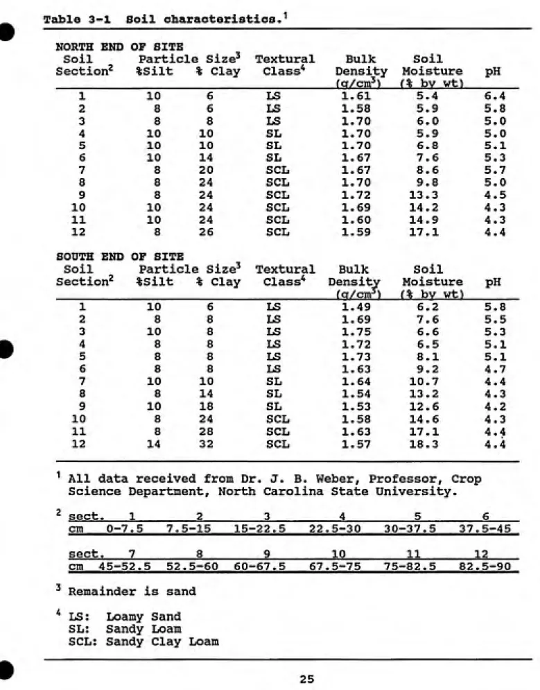
segments ranged between 3 and 4 kilograms. Soil properties as a function of depth and field location are shown in Table
3-1. The soil sections for laboratory use were air dried
for 1 week, sieved with a 2 mm standard sieve and stored in
Table 3-1 Soil characteristics. 1
NORTH END OF SITE
Soil Particle Size^ Textural Bulk Soil
Section^ %Silt % Clay Class* Density ra/cm')
Moisture r% bv wt)
PH
1 10 6 LS 1.61 5.4 6.4
2 8 6 LS 1.58 5.9 5.8
3 8 8 LS 1.70 6.0 5.0
4 10 10 SL 1.70 5.9 5.0
5 10 10 SL 1.70 6.8 5.1
6 10 14 SL 1.67 7.6 5.3
7 8 20 SCL 1.67 8.6 5.7
8 8 24 SCL 1.70 9.8 5.0
9 8 24 SCL 1.72 13.3 4.5
10 10 24 SCL 1.69 14.2 4.3
11 10 24 SCL 1.60 14.9 4.3
12 8 26 SCL 1.59 17.1 4.4
SOUTH END OF SITE
Soil Particle Size' Textural Bulk Soil
Section^ %silt % Clay Class* Density fa/cm^^)
Moisture PH
(% bv wt^
1 10 6 LS 1.49 6.2 5.8
2 8 8 LS 1.69 7.6 5.5
3 -, 10 8 LS 1.75 6.6 5.3
4 8 8 LS 1.72 6.5 5.1
5 8 8 LS 1.73 8.1 5.1
6 8 8 LS 1.63 9.2 4.7
7 10 10 SL 1.64 10.7 4.4
8 8 14 SL 1.54 13.2 4.3
9 10 18 SL 1.53 12.6 4.2
10 8 24 SCL 1.58 14.6 4.3
11 8 28 SCL 1.63 17.1 4.4
12 14 32 SCL 1.57 18.3 4.4
^ All data received from Dr. J. B. Weber, Professor, Crop
Science Department, North Carolina State University.sect. 1 2 3 4 5 6
cm 0-7.5 7.5-15 15-22.5 22.5-30 30-37.5 37.5-45
sect. 7 8 9 10 11 12
cm. 45-52.5 52.5-60 60-67.5 67.5-75 75-82.5 82.5-90 ' Remainder is sand
* LS: Loamy Sand
SL: Sandy Loam
Three analytical grade herbicides, metolachlor, 2-chloro-N- (2-ethyl-6-methylphenyl) -N-
(2-iQethoxy-l-methylethyl) acetamide, atrazine, 6-chloro-N-ethyl-N'-(l-methylethyl)-l,3,5-triazine-2,4-diamine, and primisulfuron,
3- (4,6-bis (dif luoromethoxy) -pyrimidin-2-yl) -1-
(2-methoxycarbonyl-phenylsulfonyl)-urea, were received from
CIBA Geigy Corp., Greensboro, NC. The bulk of the
laboratory studies in this project were carried out using metolachlor on colximns. Mil and M18. Properties of
metolachlor are given in Table 3-2.
Tcible 3-2 Metolachlor and its properties.
H-CH2-0-CH3
CH2CH3
C-CH2CI
Empirical Formula; Ctl5H22N02C1
METOLACHLORMolecular Wt: 283.8
Solxobility in Water: 530 mg/1
3.2 Total Organic Carbon Analysis
Total organic carbon (TOC) was measured for each of the 12
segments of columns M18, M24 and Mil and for 6 of the
segments of column M17. An Oceanographic International
Corp. TOC Analyzer was used with the following method:
• 5 gram samples were taken from each 7.5 cm soil section and ground to a powdery consistency using a mortar and
pestle.
• Smaller samples were weighed from the 5 gram sample
into glass ampules.
1 ml of distilled water was added to each ampule.
200 jLtl of 5% (by volume) phosphoric acid (HjPO^) was
added to each ampule to convert the carbonate mineralsto carbon dioxide.
• 1 ml potassium persulfate (KgSO^) was added to oxidize
the organic carbon to carbon dioxide upon heating.
• Standards were made using 1 ml potassium persulfate, 2 Ml 5% phosphoric acid and a known amount of potassium
biphthalate.
• The carbon dioxide produced from the inorganic carbon was purged with oxygen and the ampules were sealed.
• The sealed ampules were heated at 100"C for 48 hours to allow the persulfate to oxidize the organic carbon.
• Nitrogen was used to purge the carbon dioxide from the
• 10 samples of varying mass were analyzed per each soil
segment to create a plot of known carbon content v.
mass of soil. These data were fitted using linear regression with the line's slope equivalent to the
fraction of organic carbon for that soil segment.
3.3 Sorption Rate Studies
Bottle point rate studies were performed using Metolachlor on all segments of columns Mil and M18. A preliminary
3-week isotherm experiment was run to determine the soil to solution ratio necessary to allow for a 40 to 60 percent herbicide loss from solution phase. From this experiment it was determined that a 2:1 soil mass (g) to solution volume
(ml) would be necessary for all segments except the
uppesrmost segment for which a 1:1 soil to solution ratio could be used. The rate experiments were run as follows:
24 bottle reactors (40 ml Kimax* glass centrifuge
bottles) allowing for duplicates of 12 samples, were prepared for each soil segment. Each sample contained
the same soil mass.
6 blanks containing no soil were set up to allow for
accurate measurement of the initial concentration, C^,.
12 blanks containing no soil were carried along to be analyzed at each time step for comparison with the
• The bottles were prewet with a distilled water solution
of .005M sodium azide (NaNj) and .005M calcium chloride
dihydrate (CaClj'HgO) and allowed to hydrate overnight.
• A measured volume of the same sodium azide/calciumchloride solution spiked with herbicide was added the next day to create the desired soil to solution ratio
at the desired C„.o
• The reactors were t\ambled to maintain completely mixed
conditions until each pair was removed for solution
phase analysis at specified times throughout the
experimental time period.
3.4 Sorption Eguilibritim Studies
The isotherm experiments were prepared in a similar manner
as the rate experiments. An extended time period, based on
rate study analysis, was allowed for the completely mixed
batch reactors (CMBR) to reach equilibrium. The equilibrium studies were run with 10 different concentrations of
Metolachlor on all segments of columns Mil and M18 at 24±5°C
as follows:
A known and equal amount of soil was weighed into the
centrifuge tube, prewet and hydrated as described above.
• The 10 known concentrations of herbicide were added to
• 4 blanks were dedicated to measuring each initial
concentration and 2 blanks per initial concentration
were carried along to the end for comparison.
• The reactors were tumbled end over end to maintain
completely mixed conditions and then removed at the
same time for solution phase analysis.
3.5 Analytical Methods
Analysis of solution phase concentration of metolachlor was
carried out by isolating the supernatant from the soil, extracting it into hexane and using gas chromatography (GC)
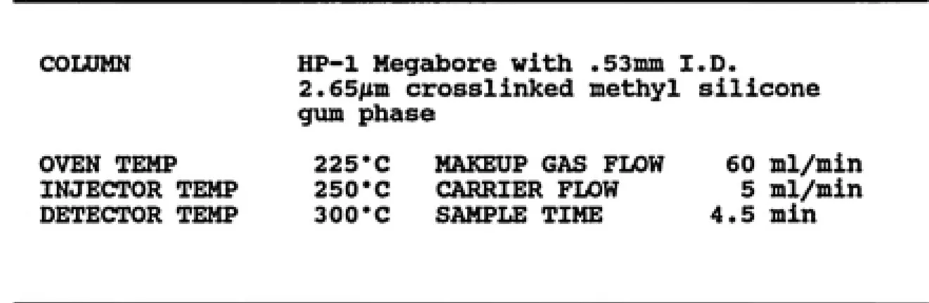
to quantify the concentration. GC settings are found in Table 3-2. The analytical methods were conducted as
follows:
• Upon removal from the tumbler, the CMBR's were
centrifuged at 1500 g's for 30 minutes to separate the soil from the supernatant.
3 ml of supernatant were extracted into 6 ml of analytical grade hexane that had been spiked with
hexachlorobenzene as an internal standard.
GC analysis was performed using an electron capture
detector on a Hewlett Packard 5890A gas chromatograph and a Hewlett Packard 3396A integrator.
Each sample was injected twice and the ratios of the
Table 3-3 6C settings.
COLUMN HP-1 Megabore with .53inm I.D.
2.65/Ltm crosslinked methyl silicone
gum phase
OVEN TEMP 225"C MAKEUP GAS FLOW 60 ml/min INJECTOR TEMP 250"C CARRIER FLOW 5 ml/min
lY EXPERIMEHTAL RESULTS USD DISCUSSIOH
4.1 Introduction
The intent of the laboratory work of this study was to
determine the soil sorption properties in 2 soil columns
taken from a field site near Clayton, NC. The 2 columns
were broken up into 12 segments each for a total of 24
different soil samples for testing. Because of its
importance in the sorption process, soil organic carbon was
analyzed early in the experimental studies followed by
sorption rate studies and sorption equilibrium studies.
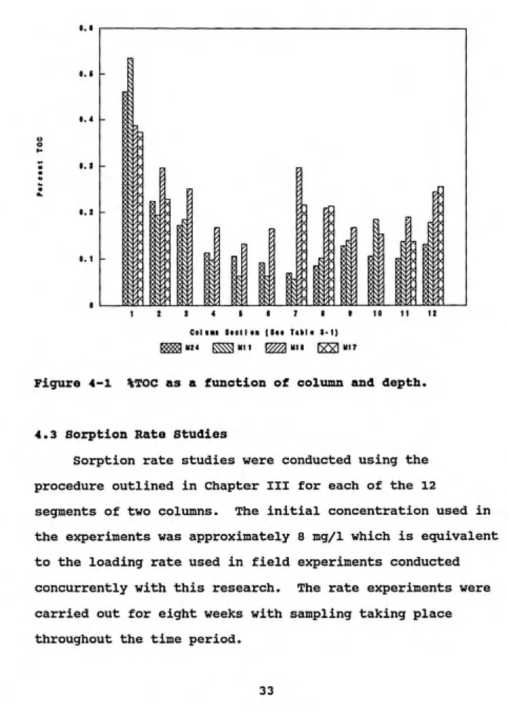
4.2 Organic Carbon Analysis
Samples from each of the 12 segments of the two columns
were analyzed for total organic carbon content (TOC). TOC
was found to vary with depth and field location, as can be
seen in Figure 4-1. TOC was highest near the soil surface
as would be expected from decaying plants and microorganism
activity. TOC decreases steadily from the surface and
reaches its minimum at about 30 to 45 cm below the surface.
The TOC in column M18 was higher than that of column Mil in
most cases. This may be due to the 1 percent grade between
the north and the south ends of the site leading to runoff
0. I
s
Csl ͣmi Stetlon ($•• Ttbl • S-1)
^1124 ^mi ^«1l ^«17
Figure 4-1 %TOC as a function of colunm and depth.
4.3 Sorption Rate studies
Sorption rate studies were conducted using the
procedure outlined in Chapter III for each of the 12
segments of two columns. The initial concentration used in
the experiments was approximately 8 mg/l which is equivalent
to the loading rate used in field experiments conducted
concurrently with this research. The rate experiments were
carried out for eight weeks with sampling taking place
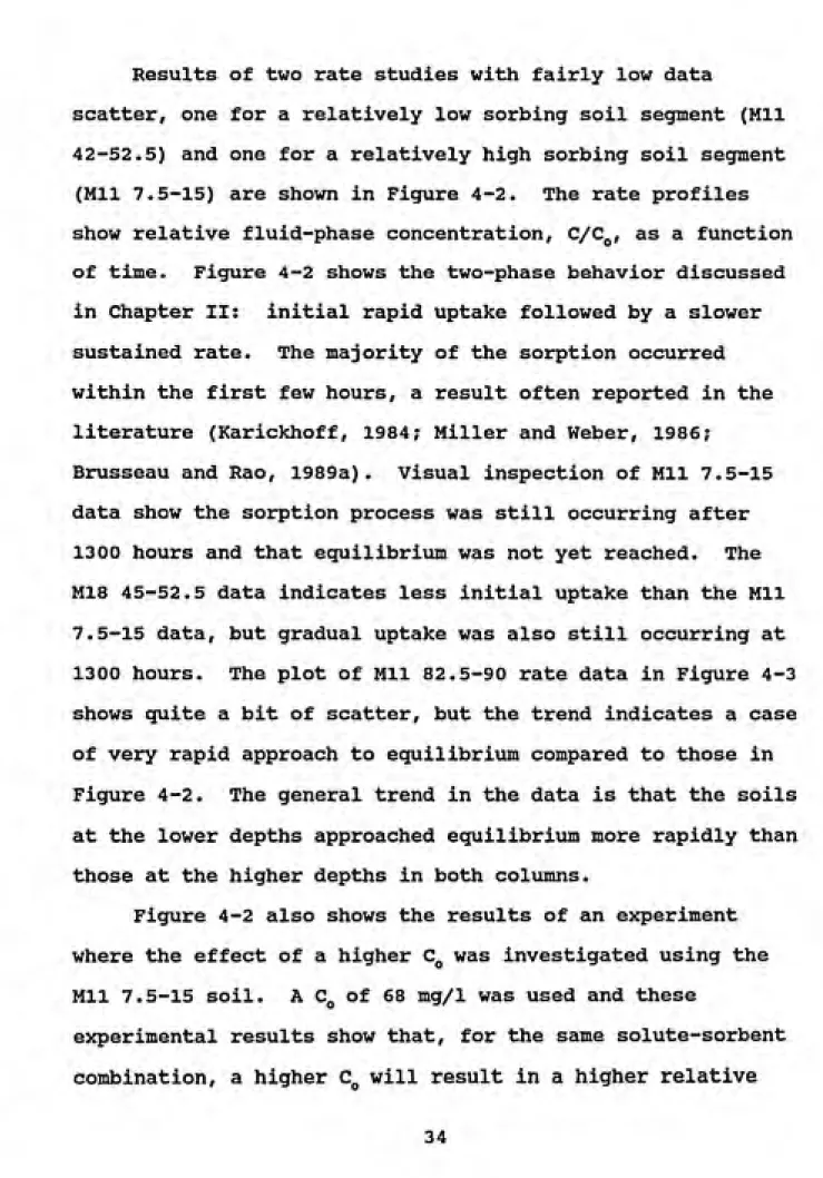
Results of two rate studies with fairly low data
scatter, one for a relatively low sorbing soil segment (Mil
42-52.5) and one for a relatively high sorbing soil segment
(Mil 7.5-15) are shown in Figure 4-2. The rate profiles
show relative fluid-phase concentration, C/C^j, as a function
of time. Figure 4-2 shows the two-phase behavior discussed
in Chapter II: initial rapid uptake followed by a slower
sustained rate. The majority of the sorption occurred
within the first few hours, a result often reported in the
literature (Karickhoff, 1984; Miller and Weber, 1986;
Brusseau and Rao, 1989a). Visual inspection of Mil 7.5-15
data show the sorption process was still occurring after
1300 hours and that equilibrium was not yet reached. The
M18 45-52.5 data indicates less initial uptake than the Mil
7.5-15 data, but gradual uptake was also still occurring at
1300 hours. The plot of Mil 82.5-90 rate data in Figure 4-3
shows quite a bit of scatter, but the trend indicates a case
of very rapid approach to equilibrium compared to those in
Figure 4-2. The general trend in the data is that the soils
at the lower depths approached equilibrium more rapidly than
those at the higher depths in both columns.
Figure 4-2 also shows the results of an experiment
where the effect of a higher C^ was investigated using the
Mil 7.5-15 soil. A C^ of 68 mg/1 was used and these
experimental results show that, for the same solute-sorbent
1.00
0.90
0.80
o
o 0.70
0.60
0.50
8 o
SB
ooooo 7.5—15 Co &i^A&& 7.5—15 Co
ͤ
nDDD 45—52.5 Co
7.1 mg/l 68.0 mg/l
7.4 mg/l
500 1000 1500
Time (hrs)
2000
Figure 4-2 Metolachlor kinetic data. Mil column.
1.00
0.90
o
o
o
0.80
0.70
0.60
Metolachlor Mil 82.5-90
Co = 7.1 mg/l
0 500 1000 1500
Time (hrs)
concentration over time. The concentration dependence of
C/Cjj would indicate a favorable nonlinear equilibrivim
distribution as is discussed in the next section.4.4 Sorption Equilibrium studies
The equilibrivim distributions between solute
fluid-phase and solid-fluid-phase concentrations for all 24 soil
segments were determined by conducting isothermal
equilibrium experiments as outlined in Chapter III. The
equilibrium distributions were achieved by keeping the soil
to solution ratios constant while varying the initial solute
concentrations between 1 mg/1 and 200 mg/1. In general, the
reactors were allowed 1000 to 1100 hours to reachequilibrium. The results of the rate studies however,
indicate that this time allotment is not sufficient in most
cases for the reactors to reach equilibrium.
As predicted from the data in Figure 4-2 for the two
Mil 7.5-15 rate experiments, the equilibrium distribution
relationships for metolachlor on these soils appear to be
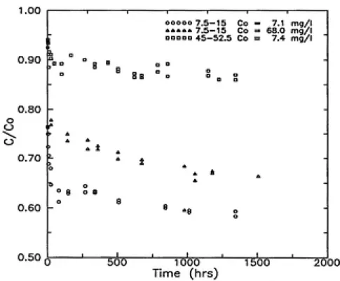
nonlinear. The Freundlich Model was used to describe theexperimental relationships. The data were plotted using the
linearized version of the Freundlich equation (Equation
2.11) and the empirical constants, K^ and n^, were obtained
from the linear regression in log space. Table 4-1 shows
Table 4-1 Freundlicli parameters and rate constants.
Mll^ Kf Standard^ "f Standard
VR^,
fcmVa)"* Error Error mr-h
1 .1770 .0981 .872 .0110 1.08*10'^
2 .0462 .0960 .833 .0131 6.82*10"^
3 .0664 .0971 .892 .0106 3.48*10"'
4 .0138 .1846 .790 .0255 1.32*10-*
5 .0415 .1662 .926 .0186 3.98*10-'
6 .0180 .2071 .855 .0294 4.25*10'
7 .0240 .1467 .881 .0163 3.49*10''
8 .0369 .2177 .906 .0311 1.03*10"*
9 .0879 .2833 .935 .0342 1.82*10-2
XO .0615 .1757 .906 .0249 2.64*10-'
11 .1039 .1507 .968 .0169 7.14*10"'
12 .1862 .1030 1.049 .0184 9.91*10-°
M18^
^f .
Standard^ "f StandardDs/R^ ,
fcmVa)"* Error Error
'hr-')
1 .1265 .0514 .851 .0072 1.39*10-2
2 .0644 .0679 .828 .0108 7.96*10"'
3 .0404 .1025 .822 .0135 4.27*10-'
4 .0446 .1209 .865 .0201 8.58*10"*
5 .0458 .1086 .902 .0150 7.45*10"*
6 .0526 .1024 .893 .0172 6.70*10"' 7 .0709 .0762 .872 .0102 1.11*10"2
8 .1982 .1069 .976 .0183 2.19*10"2 9 .1446 .0563 .964 .0085 9.14*10"2 10 .1073 .0922 .972 .0158 6.36*10"2
11 .0730 .1125 .932 .0156 1.25*10"2
12 .1181 .1561 .975 .0268 1.32*10"2
Pianatello and Huana, 1991
Soil O.C.
rL/ka^"f
Std n, Std
a/ka Err Err
Cva 23.7 10.0 3.6 0.81 0.06
Cvb 16.5 2.0 1.3 0.95 0.11
Wl 9.1 0.5 0.8 1.14 0.25
W2 6.0 0.8 0.6 0.99 0.12
^ See Table 3-1.
the log fit. The Freundlich exponent ranged from 0.79 to
1.04. Pignatello and Huang (1991) reported Freundlich
exponents for Metolachlor on 4 soils to range from 0.81 to
1.14. This data is also reported in Table 4-1.
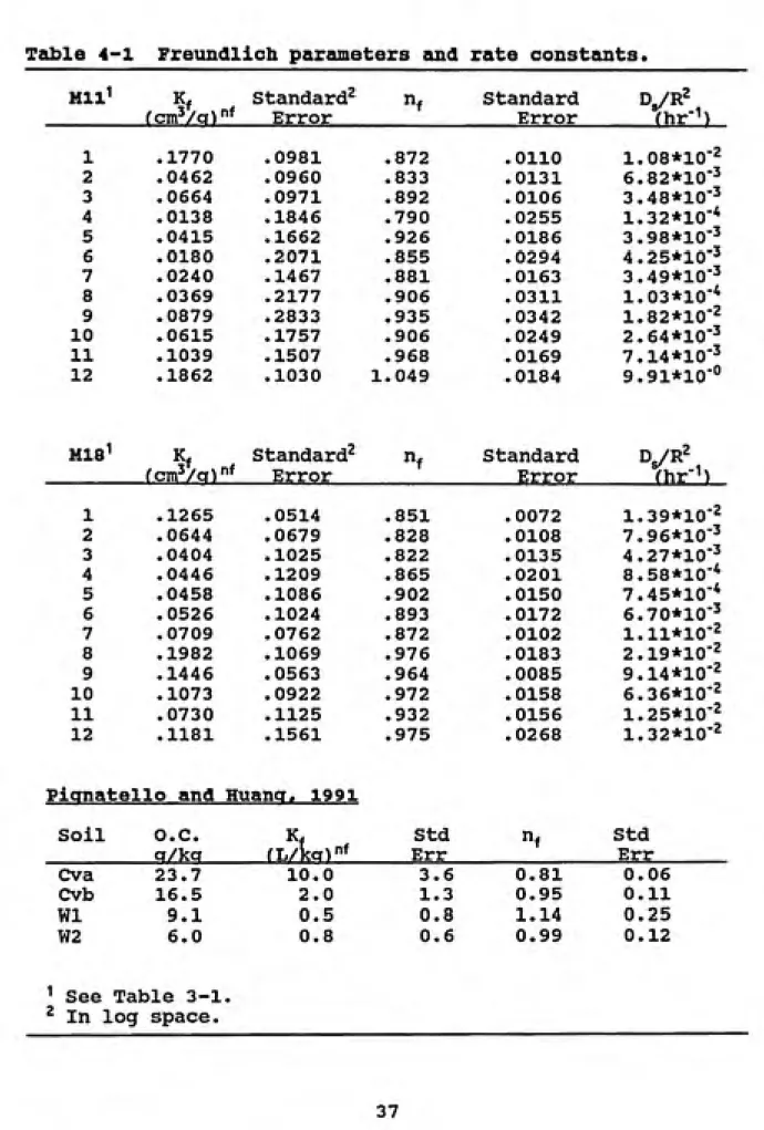
The data and Freundlich fits for the same soils for
which rate data were shown in Figure 4-2, Mil 7.5-15 and Mil
45-52.5, as well as the nearly linear case of MIS 52.5-60
are shown in Figure 4-4.
0.04
0.03
,E 0.02
<u
0.01
0.00
-I---1---r
Metolachlor M18 52.5-60
Ml 1 7.5-15 Ml 1 45-52.5
200
100 150
Ce (mg/l)
Figure 4-4 Metolachlor equilibrium data and Freundlich fits.
The large amount of data obtained in these experiments
allows one to investigate the correlation between soil
organic carbon content and the linear sorption partition
coefficient. This was accomplished by assuming the
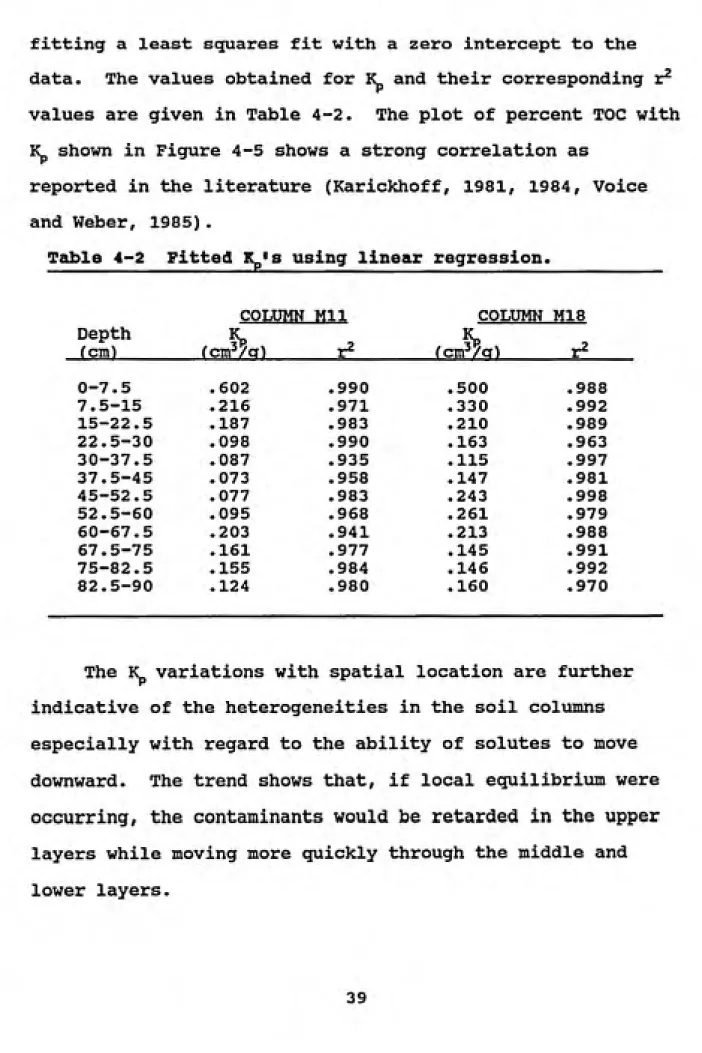
fitting a least squares fit with a zero intercept to the
data. The values obtained for K and their corresponding r^
values are given in Table 4-2. The plot of percent TOC with
Kj shown in Figure 4-5 shows a strong correlation as
reported in the literature (Karickhoff, 1981, 1984, Voice
and Weber, 1985).
Table 4-2 Fitted K^s using linear regression.
COLUMN Mil COLUMN M18
Depth (cm)
K
fcm^/a) r2
fcm^a)
r20-7.5 .602 .990 .500 .988
7.5-15 .216 .971 .330 .992
15-22.5 .187 .983 .210 .989
22.5-30 .098 .990 .163 .963
30-37.5 .087 .935 .115 .997
37.5-45 .073 .958 .147 .981
45-52.5 .077 .983 .243 .998
52.5-60 .095 .968 .261 .979
60-67.5 .203 .941 .213 .988
67.5-75 .161 .977 .145 .991
75-82.5 .155 .984 .146 .992
82.5-90 .124 .980 .160 .970
The K variations with spatial location are further
indicative of the heterogeneities in the soil columns
especially with regard to the ability of solutes to move
downward. The trend shows that, if local equilibrium were
occurring, the contaminants would be retarded in the upper
layers while moving more quickly through the middle and
0.8 0.6 en E 0.4 o CL is:
0.2
-0.
9).b
\-1 \-1 ... I \-1
o o o o o Kp data
--- Regression -...1
line
1--- ͣI...T---1"
-J
- Koc = 104 oJ
\-
o^ \
[- A
[ͣ
O
o
A
[- o ° >^ o o
H
t~
1 1 1 1 1 1 1 , 1 1 1
0.1 0.2 0.3 0.4
Percent TOC
0.5 0.6
Figure 4-5 K^ v. %TOC for metolachlor on 24 soils.
TeQ>le 4-3 Reported K 's for metolachlor.
AUTHOR Minimum Maximum Mean
Peter and Weber,
1985
116 278 198
Pignatello and Huang,
1991
88 141 121
Bouchard et al,
1982
263 269 266
Gerstl,
1990
258
Following the discussion in Chapter II, the slope of
the line in Figure 4-5 corresponds to K^,^ and has a value of
104. This shows good agreement with values reported in the
literature as shown in Table 4-3.
4.5 Modeling of Experimental Data
A dual-resistance surface-diffusion model (Pedit 1988)
was used to model experimental sorption rate data. The
intent of the modeling was to estimate a surface-diffusion
coefficient that could be used to predict sorption kinetics
in the advective-dispersive-reactive transport equation.
The modeling attempts had mild success as can be seen in
Figures 4-6 through 4-8. The model, discussed in Chapter
II, uses an iterative procedure to solve for the sorption
rate constant, D^/R^, that best fits the experimental rate
data. Dg is the surface-diffusion coefficient and R^ is the
diffusive path length. It finds D^/R^ by minimizing the
sums of square errors (SSE) between the data and the
prediction. The Freundlich isotherm parameters are input to
the model for equilibrium definition. Some of the model's
misprediction arises from the discrepancy between the
experimental equilibrium parameters and the actual
"equilibrium" attained by the rate data to be fit. Other
problems probably occur due to data scatter.
In Figure 4-6, the model predicts nearly instantaneous
1.00 0.90 -o O O 0.80 0.70 -0.60 Metolachlor f" 82.5-90
oo o oo Raw Data
H
^ Model H
L I a ho H
i
o A o 8 o o e h o Al-1 l-1 l-1 1 1
A
500 1000
Time (hrs)
Figure 4-6 Diffusion rate model fit, M18 33-36.
1500 1.00 0.90 o o '^ o 0.80 0.70 Metolachlor 22.5-30 o o o o o Raw Date
--- Surface—Diffusion Model
500 1000
Time (hrs)
1500
1.00 0.90 o o 0.80 -0.70 0.60
1 ... 1 ... 1 -ͣͣͣ 1 — ͣ
Metolachlor
L Mil 37.5-45
1-f 8 ͣ :
ͣ
i
loV
o
\- o A
Y A
1 ooooo Raw Data
1 --- Surface—Diffusion Model
1 1 1 1 1 1
A
500 1000
Time (hrs)
1500
Figure 4-8 Diffusion rate model fit/ Mil 37.5-45.
rate constant has been predicted to be quite fast such that
the model predicts the early rate data points with some
accuracy, but it misses the large time points because the
equilibrium distribution relationship predicted by the
isotherm experiments shows a higher C^ than the rate data.
In contrast, the model fit of Mil 22.5-30 in Figure 4-7 has
a much slower sorption rate constant and is not near
equilibrium at 1300 hours. Finally, Figure 4-8 shows a fit
to the Mil 37.5-45 data where the equilibrium conditions are
fairly well met, but the early time kinetics are not. This
is likely due to data scatter. The fitted D^/R^ parameters
An inverse relationship between sorption rate constant
and K^ has been reported in the literature (Brusseau and
Rao, 1989a; 1989b; Karickhoff, 1984). While not shown here,
the K and D^/R^ data in this research showed no such
relationship. The lack of correlation may be due to the
fact that R is unknown (a plot of IC with D^ might show the
predicted inverse relationship) or it may be due to some of
the poor model fits.
Following Brusseau and Rao (1989a), intraorganic matter
diffusion is likely the cause of sorption nonequilibrium for
hydrophobic organic compounds. It is the result of
rate-limited mass transfer of sorbate from the exterior
surface of the organic matter into the interior matrix. The
diffusional mass transfer is a function of three factors:the diffusivity of the diffusing species, the resistance to
diffusion associated with the sorbent matrix and thediffusion path length. A visual inspection of the
experimental rate data shows that, for these data, diffusion
path length may be an important factor. The Mil segments
below 37.5 cm showed a relatively fast approach to
equilibrium compared to those above. The same trend holds
true for the M18 segments below 60 cm. An inspection of the
Kj's (Figure 4-2) and particle textures (Figure 3-1) shows
that K 's are generally lower in these segments than the
layers. A sieve analysis would help to interpret these
trends. It would appear that the high K^'s and large
particle sizes of the higher soil segments lead to retarded
V MODELING OF FIELD DATA
5.1 Introduction
Field and experimental data were used to investigate
the predictive ability of the Pesticide Root Zone Model
(PRZM). As mentioned in Chapter II, PRZM is a management
model which uses a compartmentalized representation of the
soil profile. Details of PRZM and their relevance to this
project are discussed in this section. These details were
largely taken from the PRZM documentation source. User's
Manual for the Pesticide Root Zone Model (PRZM). Release 1.
(Carsel et al., 1984) The final portion of this section is
a discussion of modeling results.
5.2 Mass Balance
PRZM uses mass balance equations in the surface zone
and the subsurface zones to account for pesticide movement.
The mass balance in the surface zone is given by (Carsel et
al., 1984)
A^Xd(C„e) ^ ^ ^ ^ ^ ^ ^ ^ ^ P-T
for fluid-phase contaminant and
AtiXd{C,^p)
for solid-phase contaminant, where A is the cross-sectional
area of the soil column (L^), aX is the depth dimension of
the compartment (L) , C^^ is the pesticide fluid-phase
concentration (M/Ljj, C^^^ is the pesticide sorbed-phase
concentration (M/M), 6 is the soil volumetric water content
(lVl^) I P is the soil bulk density (M/L^) , t is time and the
fluxes, J (M/T), are listed in Table 5-1.
Table 5-1 Flux terms in PRZM mass balance.
J^ flux due to dispersion
Jy flux due to advection
Jpy flux due to transformation of fluid-phase
J„ flux due to plant uptake of fluid-phase
Jqp flux due to removal in runoff
Jy^p flux due to pesticide application
JpoP flux due to washoff from plants to soil
Jp5 flux due to transformation of sorbed-phase
Jgu flux due to removal on eroded recliments
J^g flux due to adsorption
Jpgg flux due to desorption
The subsurface zone mass balance is identical to Equations
5.1 and 5.2 except that the erosion, runoff and washoff from
plants terms are dropped. The applied pesticide flux term
is used in the subsurface zone mass balance only if the user
specifies that the pesticide is incorporated into the soil.
The flux terms are explained in detail in the PRZM User's
Manual. PRZM makes several assumptions when applying the
mass balance equations: the dispersion term is constant
across the horizon, all of the chemical dissolved in the
decomposition rate constant, k^, represents the sum of all
processes in both soil water and soil phases, and linear
equilibrium between phases is achieved instantaneously
(Carsel et al., 1984). The linear, instantaneous
equilibriiim assumption allows Equations 5.1 and 5.2 to be
combined by the substitution of
Equation 5.4 is PRZM's variation on the
advective-dispersive-reactive equation
- -D—r-l---3::---C^[i:^(e + iC-p) +
Ax A„Ax Ax A ^
5.4
Where the fifth term is plant uptake term, f is the fraction
of total water in the zone used for evapotranspiration (T'^)
and c is a dimensionless uptake efficiency factor. The
sixth term is the runoff term and Q^^ is the daily runoff
depth (L/T). The seventh term is the term for loss due to
erosion where X^ is the erosion sediment loss (M/T), r^ is
the enrichment ratio for organic matter (M/M), A^ is the
watershed area (L^) and a is a conversion factor. The final
term in Equation 5.4 is the pesticide application term which
is partitioned into that which is applied directly to the
soil and that which falls to the soil from the plant canopy.
F is the fraction of the application intercepted by the
rainfall depth (L/t), and IT is the mass of the pesticide on
the plant surface per cross-sectional area (M/L^) . In the
surface layer. Equation 5.4 is solved by PRZM with the plant
uptake term set to zero. In the subsurface layers within
the root zone the runoff term, the erosion term and the
application terms are set to zero and in layers below the
root zone the erosion, runoff, application, and uptake terms
are set to zero.
5.2.1 Transport Parameter Input
While PRZM was designed to handle a wide range of
agricultural scenarios, it is necessary to correctly
characterize the transport mechanisms to make accurate
predictions. Field lysimeter design prevented erosion and
runoff so they were not pertinent to these simulations.
Pesticide washoff from plant to soil was also not a
pertinent transport mechanism because the herbicide was
applied directly to the soil. The remaining mechanisms are
discussed below.
Degradation is modeled as a pseudo-first order process
and the lumped decay coefficient is input. In laboratory
degradation experiments, Braverman et al. (1986) found
metolachlor•s half-life to be between 2 and 4 weeks and
reaction products, so their continued transport is not
followed.
PRZM is one of the few models that accounts for plant
uptake. The model uses an empirical approach that assumes
that plant uptake is directly related to transpiration rate.
The user provides an efficiency factor which corresponds to
the fraction of crop transpiration associated with plant
uptake. Carsel et al. (1984) suggested that the uptake
efficiency factor may be estimated using a procedure per
Briggs et al. (1982). The efficiency factor, UPTKEFF, may
be estimated by
UPTKEFF- 0.784exp-[(Jogri<:o^-l.78)2/2.49] 5.5
For this equation, the log K^ was estimated using the
empirical of Karickhoff et al. (1979).
logJC^ - logJC^^-0.21 5.6
As presented in Chapter IV, log K^^^ was found to be 2.02,
which leads to a log K^ of 2.23 and UPTKEFF was estimated
and input into the model as 0.75.
Adsorption and desorption are handled by PRZM as
linear, reversible and instantaneous. The K values
determined in the sorption equilibrivim experiments were used
in the simulation. See Table 4-1.
PRZM accounts for dispersion using Pick's Law and
allows the user to input an effective dispersion
coefficient. Carsel et al. (1984) pointed out that the
numerical scheme chosen for the solution of the transport
equation produces numerical dispersion. The numerical
dispersion is a function of velocity and the spatial
discretization term, ax. Carsel et al. (1984) suggested
that inputting an effective dispersion coefficient will
produce a substantial amount of numerical dispersion,
however finer discretization of the soil profile will
minimize numerical dispersion. The simulations run in these
studies were run with the user input value for effective
dispersion coefficient set to zero.
5.3 Water Balance
The water balance in PRZM consists of rainfall,
snowmelt, runoff, evaporation, transpiration, and leaching.
Water balance equations are developed separately for the
surface zone, the root zone and the horizon below the root
zone. They are