Modal Analysis of the Dynamic Response of Timoshenko Beam under Moving Mass

(1)

Sharif University of Technology

Scientia Iranica

Transactions A: Civil Engineering www.scientiairanica.com

Modal analysis of the dynamic response of Timoshenko

beam under moving mass

D. Roshandel, M. Mod

_{and A. Ghannadiasl}

Department of Civil Engineering, Sharif University of Technology, Tehran, Iran. Received 9 June 2013; received in revised form 14 May 2014; accepted 3 December 2014

KEYWORDS Timoshenko beam; Moving mass; Eigenfunction expansion method; Boundary conditions; Vectorial form of orthogonality.

Abstract. In this study, the dynamic response of a Timoshenko beam under moving mass is investigated. To this end, vectorial form orthogonality property of the Timoshenko beam free vibration modes is applied to the EEM (Eigenfunction Expansion Method). The implication of the vectorial form series and an appropriate inner product of mode shapes in combination are focused for a beam with arbitrary boundary conditions. Consequently, signicant simplications and ecacy in the utilization of the EEM in eliminating the spatial domain is achieved. In order to comprise validation, the present study is compared with the DET (Discrete Element Technique) and the RKPM (Reproducing Kernel Particle Method).

1. Introduction

In recent years, all branches of transportation industry have experienced great revolutionary advances char-acterized by increasingly high speed and weight of the vehicular systems. As a result, the correspond-ing structures have been subjected to the deections and dynamic stresses far larger than ever before. The moving force/mass problems are amongst highly interested issues in the structural dynamics. The importance of the subject is manifested in numerous applications in the eld of transportation. As a matter of fact, bridges [1-6], guide-ways [7], pavements [8], overhead cranes [9], railroads [10], runways [11], and pipelines [12] are instances of structural elements in which the vibrations induced by moving inertial loads could be a signicant design factor to be considered. A rich literature on the methods and the subjects is available in [13,14] on the moving load dynamic problems.

The dynamic response of a beam to a moving force

*. Corresponding author.

E-mail address: [email protected] (M. Mod)

has been widely treated previously. However, there are clearly many problems of great physical signicance in which the mass inertia cannot be neglected. Evidently, the mass inertia causes signicant changes in the total dynamic performance of the system [15,16]. On the other hand, the thin beam theory neglects transverse shearing deformation, where this shearing eect can be accounted for through a higher order beam theory. It is noteworthy to mention that the bending modes and shear modes responses mostly appear in short beams. In 1921, Timoshenko presented a revised beam theory considering shear deformation. Considering the Timoshenko beam theory, the dynamic behavior of deep beams and the beams subjected to high-frequency excitations, would more accurately and reasonably be assessed.

Through the progressive steps towards the solu-tion of the Timoshenko beams carrying moving mass, Mackertich [17] followed Lee [18] who investigated the dynamic behavior of a Timoshenko beam subjected to an accelerating mass. Mackertich [17] represented a reasonable solution for the simply supported bound-ary conditions. He took advantage of eigenfunction expansion method taking into account the eects of

(2)

the rotary inertia. Even though, ignoring the eects of moving mass Coriolis acceleration in this study may notably conne the validity of the simulation. Lee's [18] formulation has further removed the simplifying pre-sumptions by regarding a non-permanent contact con-dition between the moving mass and the base beam during the course of the motion. Yavari, Nouri and Mod [19] tackled the dynamics of a Timoshenko beam with various boundary conditions under a moving mass by making recourse to the DET.

The vibration of a Timoshenko beam, undergo-ing arbitrarily distributed harmonic movundergo-ing load, has been explored by Kargarnovin and Younesian [20]. They regarded a beam of uniform cross-section with innite length, lying on a generalized Pasternak-type viscoelastic foundation. They solved the governing dierential equations via complex Fourier transforma-tion in conjunctransforma-tion with the residue and convolutransforma-tion integral theorems. Eftekhar Azam et al. [21] treated the motion equation of a Timoshenko beam subjected to a traveling sprung mass. They extensively compared the beam vibrations due to a moving sprung mass with those captured by the consideration of moving mass and moving force. Dyniewicz and Bajer [22] have studied this problem employing an approach similar to the eigenfunction expansion method. However, as well as other previously established solutions based on eigenfunction expansion method, their study does not include the case of a non-simply supported boundary conditions. Kiani et al. [23] have also dealt with the problem of moving mass traversing a beam by Reproducing Kernel Particle Method (RKPM) and the extended Newmark-method. They analyzed the dynamic eects of moving mass on Euler-Bernoulli, Timoshenko, and higher-order beams. The exact so-lution of Timoshenko beams using the dynamic Green function has been represented by Ghannadiasl and Mod [24].

In view of above mentioned literature on the dynamics of a Timoshenko beam under a traveling mass, the utilization of the eigenfunction expansion method has been merely constrained to the case of a simply-supported beam. On the other hand, due to the framework by which the previous researchers have followed, their numerical models lack the possibility of extending to the various boundary conditions in a favorable manner. In order to ll this gap, the presented investigations in this paper feature the main objectives of:

Presenting a very convenient, practical and robust analytical-numerical technique so as to determine the dynamic response of Timoshenko beams with various boundary conditions under the action of moving mass;

Providing guarantee of validity by including

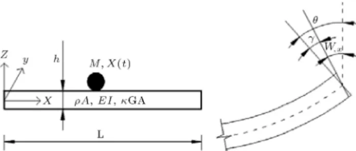
compar-Figure 1. Schematic layout of the model.

isons of the obtained results with those predicted by DET and the RKPM [19,23].

2. Problem denition

In the dynamic Timoshenko beam theory without axial eects, the displacements of the beam are assumed to be given by:

ux(x; y; z; t) = z(x; t); (1)

uy(x; y; z; t) = 0; (2)

uz(x; y; z; t) = w(x; t); (3)

where (x; y; z) are the coordinates of a point in the beam; ux, uy and uz are the components of the

displacement eld in the x, y and z directions; is the counterclockwise angle of the beam cross-section rotation, and w is the displacement of the neutral axis in the z direction as shown in Figure 1.

Using Hamilton's principle and employing the Timoshenko beam theory, one can obtain the governing dierential equations as follows [18,25]:

GA(w;xx ;x) Aw;tt= Nm

X

k=1

Mk(g w0k)(x Xk(t)); (4)

EI;xx+ GA(w;x ) I;tt= 0; (5)

w0k =

d2_w

dt2 jx=Xk(t)=

w;tt+ 2w;xtX_k(t)

+ w;xxX_k2(t) + w;xXk(t)

jx=Xk(t); (6)

in which A, E, G, I, and signify cross-sectional area of the beam, the modulus of elasticity, shear modulus, cross-sectional moment of inertia, shear correction factor and beam mass per unit of volume, respectively. Nmis the number of traveling masses.

In Eq. (6), subscripts following by \," represent partial derivatives, \." denotes dierentiation with

(3)

respect to time and d2

dt2 represents complete (total)

derivative. Moreover, Xk(t) is the time dependent

position of the kth moving mass.

The common boundary conditions associated with the Timoshenko beam theory are given as follows:

8t@x = 0; x = L : EI;x= 0 or = 0;

8t@x = 0; x = L : GA(w;x ) = 0 or w = 0: (7)

For a linear elastic three-dimensional system, free vibration modes can be written in a vectorial form as:

~

M(n)_{(x; y; z) =(U}(n)

1 (x; y; z); U2(n)(x; y; z);

U₃(n)(x; y; z)): (8) The inner product of any two modes can be dened as follows:

~

M(i)K_M_~ (j)₌Z Z Z V

~

M(i)_{: ~}_M(j)_dV

= Z Z Z

V(U (i)

1 U1(j)+ U2(i)U2(j)

+ U₃(i)U₃(j))dV: (9) Any two diverse modes of a linear elastic media have the orthogonality property with respect to the inner product in Eq. (9) [26], that is:

i 6= j ! ~M(i)K_M_~ (j)_{= 0:} ₍₁₀₎

For instance, this characteristic could be applied to evaluate the accuracy of experimentally determined natural modes. In the present research, it allows expressing a general solution of the forced vibration equation in terms of an innite series of modes. By using the displacement eld according to Timoshenko beam theory, free vibration modes can be written in a vectorial form as:

~

M(n)_{= (}

nz; 0; n): (11)

In Eq. (11), n and n stand for the nth mode shape

corresponding to transverse deection and rotation, re-spectively. Furthermore, nand nare both functions

of x. In a summarized form: ~

M(n)_{= (}

nz; n): (12)

In the specic case of Timoshenko Beam theory, the inner product of two modes can be dened as follows:

~

M(i)K_M_~ (j)₌Z l 0

ZZ

A

( iz; i):( jz; j)dAdx

= Z _l

0

ZZ

A

(ij+ i jz2)dAdx

= Z _l

0 (Aij+ I i j)dx: (13)

Ultimately, by using the orthogonality of natural modes and normalizing mode shapes, Eqs. (10) and (13) will lead to:

Z _l

0 (Aij+ I i j)dx = ij; (14)

wherein, ij is the Kronecker delta function as:

ij=

8 < :

1; i = j 0; i 6= j

It should be highlighted that i, j, i and j are

not orthogonal except in the case of hinged-hinged boundary conditions. In other words, if i 6= j, then R_l

0(i) (j)dx,

R_l

0 (i) (j)dx and

R_l

0(i)(j)dx are not

necessarily equal to zero excepting the case of a simply supported beam. The form of general orthogonality, which is valid for all boundary conditions, is the one stated in Eqs. (12) and (14) in which, as mentioned before, has a vectorial format. This is the key point which makes the solutions in this paper distinct from the other corresponding ones presented in the available literature.

3. The method of the solution

Free vibration modes of a Timoshenko beam could be derived from the following equations:

GA(w;xx ;x) Aw;tt= 0; (15)

EI;xx+ GA(w;x ) I;tt= 0: (16)

Eqs. (15) and (16) could be handled using direct separation of variables:

w(x; t) = (x) (t);

(x; t) = (x) (t): (17)

It should be noted that in the case of free vibration, and should have the same coecient [29]. By in-troducing Eq. (17) to Eqs. (15) and (16), the following equations could be derived straightforwardly:

(4)

(EI (x);xx+ GA ((x);x (x))) (t)

I (x)(t) = 0: (19)

For Eqs. (16) and (17) to be separable, (t)_(t) must be constant, therefore:

;tt _{= ^!}2_{! (t) = A sin(^!t) + B cos(^!t);} ₍₂₀₎

wherein ^! is the natural frequency of free vibration. Regarding !4

j = AEI^!2j and substituting Eq. (20) into

Eqs. (18) and (19) end in the following equations: GA (j;xx(x) j;x(x)) + EI!4jj(x) = 0; (21)

EI j;xx(x) + GA (j;x(x) j(x))

+EI_A2!4

j j(x) = 0: (22)

According to Eqs. (4) and (5), the vectorial form of the governing dierential equation is as follows:

GA(w;xx ;x) Aw;tt; EI;xx+ GA(w;x )

I;tt

= XNmMk(g w0k)(x Xk(t)); 0

! :

(23) w(x; t) and (x; t) could be expanded in terms of and :

(w(x; t); (x; t)) =X1

j=1

(j(x); j(x)) Tj(t): (24)

Considering the rst n free vibration mode shapes, Eqs. (6) and (24) could be substituted into Eq. (23) arriving at:

n

X

j=1

GA(j;xx(x) j;x(x))Tj(t) Aj(x) Tj(t);

EI j;xx(x)Tj(t) + GA(j;x(x) j(x))

I j(x) Tj(t)

=

n

X

j=1

XNm

=1

M[g (j(x) Tj(t)+2j;x(x) _Tj(t) _X(t)

+ j;xx(x)Tj(t) _X2(t) + j;x(x)Tj(t)

X(t))]jx=X(t)(x X(t)); 0

: (25) !j is dened as:

!4

j = A_EI^!2j; (26)

where ^!j is the frequency of the jth free vibration

mode. According to Eqs. (21) and (22) and the denition of !j in Eq. (26), it is evident that:

GA(j;xx j;x) = EI!j4j and

EI j;xx+ GA(j;x j) = EI 2

A !j4 j: (27) Therefore Eq. (25) would take a simpler form:

n

X

j=1

EI!4

jj(x)Tj(t) Aj(x) Tj(t);

EI2

A !j4 j(x)Tj(t) I j(x) Tj(t)

= n j=1

Nm

k=1Mk[g (j(x) Tj(t)

+ 2j;x(x) _Tj(t) _Xk(t)

+ j;xx(x)Tj(t) _Xk2(t) + j;x(x)Tj(t)

Xk(t))]jx=Xk(t)(x Xk(t)); 0

: (28) Performing an inner product of (i(x); i(x)) on

Eq. (28) and integrating both sides of the resulting equation with respect to x over the length of the beam (0 x L) result in:

n

X

j=1

Z x=L

x=0 (Aj(x)i(x) + I j(x) i(x))dx

!

EI

A !j4Tj(t) + Tj(t)

=

Z _x=L

x=0 n

X

j=1

XNm

k=1

Mk(g

j(x) Tj(t) 2j;x(x) _Tj(t) _Xk(t)

j;xx(x)Tj(t) _Xk2(t) j;x(x)Tj(t)

Xk(t))j_x=Xk(t)i(x)(x Xk(t))

: (29)

By applying the orthogonality condition from Eq. (14), for linear elastic, isotropic, and homogeneous beam of constant cross-section, the integral in the left side of Eq. (29) could be highly simplied taking the form of P

(EI

A!4jTj(t) + Tj(t))ij in which the voluminous

(5)

side of Eq. (29) can be simplied using characteristics of Dirac delta. So Eq. (29) could be rewritten as follows:

EI

A !j4Tj(t) + Ti(t) =

n

X

j=1 Nm

X

k=1

Mk(gi(x)

i(x)j(x) Tj(t) 2i(x)j;x(x) _Tj(t) _Xk(t)

i(x)j;xx(x)Tj(t) _Xk2(t) i(x)j;x(x)Tj(t)

Xk(t))j_x=Xk(t)Hk(t)

; (30)

wherein Hk(t) is dened as:

Hk(t) =

8 < :

1 0 < Xk(t) < L

0 Xk(t) < 0 or Xk(t) > L

(31) It would be interesting to point out that in the solution of Euler-Bernoulli beam equation via eigenfunction expansion method, after elimination of the spatial domain, an expression similar to Eq. (30) could be derived; however it is dierent because ! and are not the same as those in thin beam equation. It should be underlined that even in the case of a hinged-hinged beam in which is the same in both theories, ! is dierent and this, in turn, makes the total equations dierent. Besides, as shown in Section 4.2, this formulation gives dierent results compared to thin beam theory. Eq. (30) could be rearranged as follows:

n

X

j=1

Mij(t) Tj(t) + n

X

j=1

Cij(t) _Tj(t) + n

X

j=1

Kij(t)Tj(t)

= fi(t): (32)

Reproducing the equations, in a matrix version, results in:

[M(t)]nn:[ T (t)]n1+ [C(t)]nn:[ _T (t)]n1

+ [K(t)]nn:[T (t)]n1= [f(t)]n1: (33)

Eq. (33) is a set of n equations with n unknowns which can be solved through a numerical procedure [27,28]. The (i; j)th element of the matrices in Eq. (33) is as follows:

Mij(t) = ij+ Nm

X

k=1

Mki(Xk(t))j(Xk(t))Hk(t);

(34) Cij(t)=

Nm

X

k=1

2Mki(Xk(t))j;x(Xk(t)) _Xk(t)Hk(t)

; (35)

Kij(t) =EI 2

A !j4ij+ Nm

X

k=1

Mki(Xk(t))

j;xx(Xk(t)) _Xk2(t)+j;x(Xk(t)) Xk(t)

Hk(t)

; (36)

fi(t) = Nm

X

k=1

(Mkgi(Xk(t))Hk(t)) : (37)

To carry out the computations, one should apply the natural mode shapes of the beam to Eqs. (34)-(37) in order to form the matrices presented in Eq. (33). Though, having been discussed in the literature previ-ously [29], the mode shapes of Timoshenko beam are given in the appendix of this paper to facilitate the reproduction of the presented calculations.

To make a comparison between the presented method herein and the conventional ones [18,21], let us assume that the coecients of and are dierent:

w(x; t) =

1

X

j=1

j(x)Tj(t);

(x; t) =X1

j=1

j(x)j(t): (38)

Considering the rst n modes of free vibration and applying Eq. (38) to Eqs. (4) and (5) result in:

n

X

j=1

GA(j;xx(x)Tj(t) j;x(x)j(t))

Aj(x) Tj(t)

=Xn

j=1

XNm

k=1

Mk[g

(j(x) Tj(t) + 2j;x(x) _Tj(t) _Xk(t)

+ j;xx(x)Tj(t) _Xk2(t)

+ j;x(x)Tj(t) Xk(t))]jx=Xk(t)(x Xk(t)); 0

; (39)

1

X

j=1

EI j;xx(x)j(t) + GA(j;x(x)Tj(t)

j;x(x)j(t)) I j(x)j(t)

= 0: (40) Considering the rst n mode shapes of free vibration and multiplying both sides of Eqs. (39) and (40) by

(6)

i(x) and i(x), respectively, then integrating the

resulting equations with respect to x over the length of the beam, one could arrive at:

n

X

j=1

GA Z _L

0 i(x)j;xx(x)dx

! Tj(t)

n

X

j=1

GA Z _L

0 i(x) j;x(x)dx

! j(t) n X j=1 A Z _L

0 i(x)j(x)dx

! Tj(t)

= n X j=1 Nm X k=1 Mk

gi(x) i(x)j(x) Tj(t)

2i(x)j;x(x) _Tj(t) _Xk(t) i(x)j;xx(x)Tj(t)

_ X2

k(t) i(x)j;x(x)Tj(t) Xk(t)

j_x=Xk(t)Hk(t)

; (41) n X j=1 GA Z _L

0 i(x)j;x(x)dx

! Tj(t)

+Xn

j=1

(EI Z _L

0 i(x) j;xx(x)dx

GA Z _L

0 i(x) j(x)dx)j(t) n

X

j=1

I Z _L

0 i(x) j(x)dx

!

j(t) = 0: (42)

The matrix version of the set of coupled second-order ODEs in Eqs. (41) and (42) could be stated as:

[M(11)_]

nn [M(12)]nn

[M(21)_]_nn _[M(22)_]_nn

2n2n

:

[ T ]n1

[]n1

2n1

+

[C(11)_]_nn _[C(12)_]_nn

[C(21)_]

nn [C(22)]nn

2n2n

:

[ _T ]n1

[ _]n1

2n1

+

[K(11)_]

nn [K(12)]nn

[K(21)_]

nn [K(22)]nn

2n2n

:

[T ]n1

[]n1

2n1

=

[f(1)_] n1

[f(2)_]_n1

2n1

: (43)

The elements of matrices in Eq. (43) are as follows:

M_ij(11)(t)= A Z _L

0 i(x)j(x)dx Nm

X

k=1

Mki(Xk(t))

j(Xk(t))Hk(t);

M_ij(12)= 0; M_ij(21)= 0;

M_ij(22)= I Z _L

0 i(x) j(x)dx; (44)

C_ij(11)(t) =

Nm

X

k=1

2Mki(Xk(t))j;x(Xk(t))

_

Xk(t)Hk(t)

;

C_ij(12) = 0; C_ij(21)= 0; C_ij(22)= 0; (45)

K_ij(11)(t) =GA Z _L

0 i(x)j;xx(x)dx Nm

X

k=1

Mki(Xk(t))(j;xx(Xk(t))

_ X2

k(t) + j;x(Xk(t)) Xk(t))Hk(t)

; K_ij(12) = GA

Z _L

0 i(x) j;x(x)dx;

K_ij(21) = GA Z _L

0 i(x)j;x(x)dx;

K_ij(22) =EI Z _L

0 i(x) j;xx(x)dx

GA Z _L

0 i(x) j(x)dx: (46)

f_i(1)(t) =Xn

j=1 Nm

X

k=1

f Mkgi(x)Hk(t)g ;

f_i(2)(t) = 0: (47)

Disregarding the vectorial orthogonality of mode shapes and assuming dierent coecients for i(x)

and i(x), as shown in Eqs. (38)-(47), lead to the

formation of a set of 2n second order ODEs instead of a set of n second order ODEs (Eq. (33)). Moreover, except the case of hinged-hinged boundary condition, the integrals in Eqs. (44)-(47) are not necessarily zero when i 6= j; therefore, more computational eort is required to calculate the elements of matrices in

(7)

Eq. (43) compared to Eq. (33). Some numerical examples are solved in the next section that shows the method presented through Eqs. (15) to (37) leads to satisfactory correspondence with two other numerical solutions; furthermore, it is shown that following the alternative method presented through Eqs. (38)-(46) ends in almost the same results for the deection and the rotational angle of Timoshenko beam.

It is notable that, an equivalent method to the one presented in Eqs. (38)-(46) is decoupling the governing dierential equations of Timoshenko beam [18,22]. This will result in a set of n fourth order ODEs. More-over, as it is shown in a previous research work [18], the coecients of the ODEs contain many integrals, and as mentioned before, for boundary conditions other than hinged-hinged, such integrals are not necessarily zero for i 6= j.

4. Numerical examples

In this section, two sets of numerical examples are solved to compare the analysis results obtained by the method presented in Section 3 of this article with those of two other published studies using DET and RKPM. 4.1. Comparison with DET

To verify the new formulation of EEM which is dis-cussed in detail in Section 3 of this article, two numer-ical examples are solved and the results are compared with those obtained by the previously published study which utilized DET to handle the problem [29]. The beams are considered with the following characteris-tics:

Simply supported beam (SS):

L (m): 4.352 G (N/m2_{): 7:7 10}10

A (m2_{): 1:31 10} 3 _{(-): 1.43}

I (m4_{): 5:71 10} 7 _{M (kg): 21.83}

m (kg): 87.04 c (m/s): 27.49 E (N/m2_{): 2:02 10}11

Cantilever beam (CF):

L (m): 7.62 G (N/m2_{): 8:18 10}10

A (m2_{): 5:90 10} 3 _{(-): 1.2}

I (m4_{): 4:58 10} 5 _{M (kg): 525}

m (kg): 350 c (m/s): 50.8 E (N/m2_{): 2:14 10}11

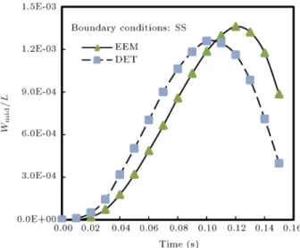
wherein, M is the moving mass, \m" represents the total mass of the beam, \c" is the moving mass velocity, \E" is the Young's modulus, \G" is the shear modulus, \I" is the moment of inertia, \A" is the beam cross-sectional area, \L" is the beam length, and \" is the shear correction factor. In Figures 2 and 3, the dynamic deections of mid-span of the SS beam and the free

Figure 2. Dynamic deection of hinged-hinged beam in numerical example mentioned in Section 4.1 (EEM curves are calculated using the rst ve modes).

Figure 3. Dynamic deection of cantilever beam in numerical example, mentioned in Section 4.1 (EEM curves are calculated using the rst ve modes).

end of CF beam, under moving mass, calculated using EEM, is compared with those obtained by DET [29]. For the simply supported beam, Figure 2 shows that the results are fairly close, and the maximum dierence is 5% for the maximum dynamic deection of mid span. Comparison of the results for the cantilever beam (Figure 4) shows that the dierence is about 15%; however, as it is shown in the next numerical study, the results of the present study coincide with those calculated using RKPM [23] for all common boundary conditions.

4.2. Comparison with the RKPM

In this example, the results of EEM are compared with those of RKPM [23]. To this end, considering dierent

(8)

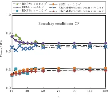
Figure 4. Dynamic deection of clamped-free beams in numerical example mentioned in Section 4.2 (EEM curves are calculated using the rst ve modes).

values for the slenderness of the beams ( = L=r) and the velocity of moving mass, a parametric study is performed to investigate the maximum deections of beams with four dierent boundary conditions, simple-simple, simple-clamped, clamped-clamped and clamped-free, and the results are compared with the analysis by RKPM [23]. The characteristics of the beams and denition of parameters used in this ex-ample are as follows.

The cross-section of the beam is assumed to be rectangular:

b : Width of the beam cross-section: b = 0:1 m

h : Height of the beam cross-section: h = p2_12r

r : Radius of gyration of the beam cross-section: r = L

L : Length of the beam: L = 10 m : Slenderness of the beam: = L=r E : Modulus of elasticity:

E = 2:1 1011 _N/m2

G : Shear modulus:

G = 8:0769 1010_N/m2

: Shear factor: = 0:833

: Density of the beam : = 7800 kg/m3

M : Moving mass: M = 0:15 AL V : Velocity of the moving mass

Wmax: Maximum deection of the beam under

the action of moving mass

W0: Maximum deection of the similar

Euler-Bernoulli beam under a static load equal to Mg

boundary

conditions : S ! Simple, C ! Clamped, F ! Free, Wmax;N =jW_Wmaxj

0 ; W0ss=

MgL3

48EI ; W0sc= 0:0098124MgL

3

EI ; W0;cc= MgL3

192EI; W0;cc=MgL

3

3EI v0= L

s EI A:

Moreover, In the CF case, moving mass is assumed to travel from the free end toward the clamped end and in the SC case, when V = 0:5 v0_{, the moving mass}

is assumed to travel from the simple end toward the clamped end, and when V = v0 _{from the clamped end}

to the simple end.

A wide range of slenderness, dierent speeds and various boundary conditions are investigated in this example. As shown in Figures 4-7, the results obtained by EEM and RKPM [23] are almost the same except in the case of cantilever beams for v = 0:5 v0_{. However,}

even in this case, the results are reasonably close. Therefore, this example could verify the eigenfunction expansion formulation used in the present study. 4.3. A clamped-simply supported beam under

successive constant moving mass

In this numerical example, the convergence rate of the method which was presented in Section 3 is investi-gated. Moreover, noticing that each mode shape of

Figure 5. Dynamic deection of simple-simple beams in numerical example mentioned in Section 4.2 (EEM curves are calculated using the rst ve modes).

(9)

Figure 6. Dynamic deection of simple-clamped beams in numerical example mentioned in Section 4.2 (EEM curves are calculated using the rst ve modes).

Figure 7. Dynamic deection of clamped-clamped beams in numerical example mentioned in Section 4.2 (EEM curves are calculated using the rst ve modes.)

Timoshenko beam contains a function that corresponds to deection of each point () and another function corresponds to rotation of each point ( ), it is shown that assuming dierent coecients for and will lead to the same results; however, as discussed in detail in Section 3, it will be more time consuming, compared to the method presented in this study.

In this numerical study, a Timoshenko beam, with Clamped-Simple (CS) boundary conditions, is considered. The excitation is assumed to be caused by a series of successive point masses moving at a constant speed (v) (Figure 8). The relative distance of the moving particles is L0 and mass of each one is M.

Figure 8. Layout of clamped-simply supported beam under successive moving masses.

Characteristics of the problem are as follows: L (m): 10 (-): 0.833 A (m2_{): 1} _{M (kg): 0:05 AL}

I (m4_{): 0.333} _L

0 (m): 0.25 L

P (kg/m3_{): 2500} _T

1(m): 0.0284

E (N/m2_{): 2 10}10 _{v (m/s): 352}

G (N/m2_{): 8:333 10}9

v0_{= L=T}₁_{and T}₁_{is the period of the rst free vibration}

mode of the beam; t _{is dened as the time taken}

by the rst travelling mass to pass the beam, so: t _{= L=v, where L is the length of the beam and v is}

the speed of moving particles. Moreover, the Dynamic Magnication Factor (DMF) is the ratio of the dynamic response of beam to the corresponding static response of it.

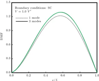
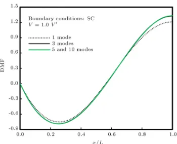
Considering both the conventional method (dif-ferent coecients for and ) and the formulation presented in Section 3, this problem is solved for v = 0:3 v0 _{and v = 1:0 v}0_{. To this end, dierent numbers}

of mode shapes were used to estimate the dynamic response of the beam. Utilizing the same number of mode shapes, the results of both methods showed to be the same. Moreover, using more than 3 modes led to the same result as shown in Figures 9-12.

The dynamic magnitude factor corresponding to the deection and rotation of dierent points along the

Figure 9. Dynamic magnitude factor corresponding to the deection of the beam in numerical example 4.3 at t = 0:8t.

(10)

Figure 10. Dynamic magnitude factor corresponding to the rotation of the beam in numerical example 4.3 at t = 0:8t.

Figure 11. Dynamic magnitude factor corresponding to the deection of the beam in numerical example 4.3 at x = L=4.

beam for v = v0 _{and at t = 0:8 t} _{are depicted in}

Figures 9 and 10, respectively. To determine the DMF curve, the dynamic response of the beam is divided by the static response assuming that moving masses are at the same position as they are when t = 0:8 t_.

Assuming v = 0:3 v0_{, DMF curves corresponding}

to the deection and rotation of the point on the beam, which is located at L=4 from the clamped edge, are depicted in Figures 11 and 12, respectively. To determine DMF, the dynamic response of the beam is divided by the maximum static response which could happen at x = L=4.

5. Conclusions

In this paper, a modied EEM formulation for dynamic analysis of Timoshenko beam was presented. It was

Figure 12. Dynamic magnitude factor corresponding to the rotation of the beam in numerical example 4.3 at x = L=4.

shown that using the vectorial form of orthogonality of mode shapes combined with an appropriate denition for the inner product of vectors enables EEM to be used for analyzing the dynamic response of Timoshenko beams of various boundary conditions in an ecient manner. Moreover, this modied formulation leads in signicant computational ecacy:

It reduces either the order or the number of the set of ordinary dierential equations which has to be solved after substituting the eigenfunctions in the governing partial dierential equation of Tim-oshenko beam. In fact it reduces either the fourth order set of n ODEs or the second order set of 2n ODEs to a second order set of n ODEs

It omits much unnecessary integration in forming the set of ODEs encountered in the eigenfunction expansion solutions.

Considering common boundary conditions, a few numerical examples were solved to verify the presented analysis approach. The comparison of the results showed a reasonable similarity with discrete element method (DET) approximations [19], while they almost matched the results of Reproducing Kernel Particle Method (RKPM) [23].

References

1. Calcada, R., Cunha, A. and Delgado, R. \Analysis of trac-induced vibrations in a cable-stayed bridge", Part I: Experimental Assessment, Journal of Bridge Engineering, 10(4), pp. 370-385 (2005).

2. Ebrahimzadeh Hassanabadi, M., Vaseghi Amiri, J. and Davoodi, M.R. \On the vibration of a thin rectangular plate carrying a moving oscillator", Scientia Iranica,

(11)

Transactions A: Civil Engineering, 21(2), pp. 284-294 (2014).

3. Eftekhari, S.A. and Jafari, A.A. \Vibration of an initially stressed rectangular plate due to an acceler-ated traveling mass", Scientia Iranica, Transactions A: Civil Engineering, 19(5), pp. 1195-1213 (2012).

4. Esen, _I. \A new nite element for transverse vibration of rectangular thin plates under a moving mass", Finite Elements in Analysis and Design, 66, pp. 26-35 (2013).

5. Nikkhoo, A., Ebrahimzadeh Hassanabadi, M., Eftekhar Azam, S. and Vaseghi Amiri, J. \Vibration of a thin rectangular plate subjected to series of moving inertial loads", Mechanics Research Communications, 55, pp. 105-113 (2014).

6. Ebrahimzadeh Hassanabadi, M., Nikkhoo, A., Vaseghi Amiri, J. and Mehri, B. \A new orthonormal poly-nomial series expansion method in vibration analysis of thin beams with non-uniform thickness", Applied Mathematical Modelling, 37(18-19), pp. 8543-8556 (2013).

7. Wang, H.P., Li, J. and Zhang. K. \Vibration analysis of the maglev guideway with the moving load", Journal of Sound and Vibration, 305.4, pp. 621-640 (2007).

8. Beskou, N.D. and Theodorakopoulos, D.D. \Dynamic eects of moving loads on road pavements: A review", Soil Dynamics and Earthquake Engineering, 31, pp. 547-567 (2011).

9. Oguamanam, D.C.D., Hansen, J.S. and Heppler, G.R. \Dynamics of a three-dimensional overhead crane sys-tem", Journal of Sound and Vibration, 242.3, pp. 411-426 (2011).

10. Chamorro, R., Escalona, J.L. and Gonzalez, M. \An approach for modeling long exible bodies with ap-plication to railroad dynamics", Multibody System Dynamics, 26.2, pp. 135-152 (2011).

11. Huang, M-H. and Thambiratnam, D.P. \Deection response of plate on Winkler foundation to moving accelerated loads", Engineering Structures, 23.9, pp. 1134-1141 (2001).

12. Yoon, Han-Ik and In-Soo Son \Dynamic behavior of cracked simply supported pipe conveying uid with moving mass", Journal of Sound and Vibration, 292.3, pp. 941-953 (2006).

13. Ouyang, H. \Moving-load dynamic problems: A tuto-rial (with a brief overview)", Mechanical Systems and Signal Processing, 25(6), pp. 2039-2060 (2011).

14. Bajer, C.I. and Dyniewicz, B., Numerical Analysis of Vibrations of Structures Under Moving Inertial Load, Springer (2012).

15. Akin, J.E. and Mod, M. \Numerical solution for response of beams with moving mass", Journal of Structural Engineering, 115(1), pp. 120-131 (1989).

16. Mod, M. and Akin, J.E. \Discrete element response of

beams with traveling mass", Advances in Engineering Software, 25(2-3), pp. 321-331 (1996).

17. Mackertich, S. \Response of a beam to a moving mass", Journal of the Acoustical Society of America, 92(3), pp. 1766-1769 (1992).

18. Lee, H.P. \Transverse vibration of a Timoshenko beam acted on by an accelerating mass", Applied Acoustics, 47(4), pp. 319-330 (1996).

19. Yavari, A., Nouri, M. and Mod, M. \Discrete element analysis of dynamic response of Timoshenko beams un-der moving mass", Advances in Engineering Software, 33(3), pp. 143-153 (2002).

20. Kargarnovin, M.H. and Younesian, D. \Dynamics of Timoshenko beams on Pasternak foundation under moving load", Mechanics Research Communications, 31, pp. 713-723 (2004).

21. Eftekhar Azam, S., Mod, M. and Afghani Khoras-ghani, R. \Dynamic response of Timoshenko beam under moving mass", Scientia Iranica, 20(1), pp. 50-56 (2013).

22. Dyniewicz, B. and Bajer, C.I. \New feature of the solution of a Timoshenko beam carrying the moving mass particle", Archives of Mechanics, 62(5), pp. 327-341 (2010).

23. Kiani, K., Nikkhoo, A. and Mehri, B. \Prediction capabilities of classical and shear deformable beam models excited by a moving mass", Journal of Sound and Vibration, 320(3), pp. 632-648 (2009).

24. Ghannadiasl, A. and Mod, M. \Dynamic green func-tion for response of Timoshenko beam with arbitrary boundary conditions", Mechanics Based Design of Structures and Machines, 42.1, pp. 97-110 (2014).

25. Fryba, L., Vibration of Solids and Structures under Moving Loads, pp. 13-33, Noordho International Publication, Prague (1973).

26. Soedel, W., Vibration of Shells and Plates, 2nd Edi-tion, pp. 106-116, Marcel Dekker, New York (1993).

27. Boyce, W.E. and Diprima, R.C., Elementary Dier-ential Equations and Boundary Value Problems, 6th Edition, pp. 339-418, John Wiley and sons, Inc. New York (1997).

28. Nikkhoo, A., Rofooei, F.R. and Shadnam, M.R. \Dy-namic behavior and modal control of beams under moving mass", Journal of Sound and Vibration, 306(3-5), pp. 712-724 (2007).

29. Van Rensburg, N.F.J. and Van Der Merwe, A.J. \Nat-ural frequencies and modes of a Timoshenko beam", Wave Motion, 44(1), pp. 58-69 (2006).

Appendix

Free vibration mode shapes of Timoshenko beam

According to Eqs. (4) and (5), to investigate the free vibration mode shapes of Timoshenko beam, the

(12)

following set of coupled equations must be solved: GA(w;xx ;x) Aw;tt= 0; (A.1)

EI;xx+ GA(w;x ) I;tt= 0: (A.2)

One can easily decouple the above equations as follows: w;xxxx _E+_G

w;xxtt+ 2

GEw;tttt+ A

EIw;tt_(A.3)=0;

;xxxx _E+_G

;xxtt+ 2

GE;tttt+ A

EI;tt= 0:_(A.4)

To nd the solution of Eqs. (A.3) and (A.4), separation of variables is an appropriate method. According to this method, we will assume:

w(x; t) = (x)T (t); (A.5)

(x; t) = (x)T (t): (A.6)

Substituting Eqs. (A.5) and (A.6) into Eqs. (A.3) and (A.4), respectively, will result in:

IV_{(x)T (t)}

E + G

II_(X)_{T (t)}

+ 2

GE(x)TIV(t) + A

EI(x) T (t) = 0; (A.7)

IV_{(x)T (t)}

E + G

II_(X)_{T (t)}

+_GE2 (x)TIV_{(t) +}A

EI (x) T (t) = 0: (A.8) Considering Eqs. (A.7) and (A.8), separation of vari-ables implies that:

T

T = constant and TIV

T = constant;

T (0) = 0 ! T (t) = A sin(^!t): (A.9) Substituting Eq. (A.9) in Eqs. (A.7) and (A.8) leads to the following equations:

IV_{+ (1 + )r}2_!400_{+ (r}4_!8 _!4_{) = 0;} _(A.10) IV_{+ (1 + )r}2_!4 00_{+ (r}4_!8 _!4_{) = 0:} _(A.11)

In the above equations: = _GE ; r2₌ I

A; !2= r

A

EI^!: (A.12) Each of Eqs. (A.10) and (A.11) has two sets of solutions as follows:

A: If ! < 1

4

p

r then:

(x) =C1sin(ax) + C2Cos(ax) + C3sinh(x)

+ C4cosh(x); (A.13)

(x) =C0

1sin(ax) + C20Cos(ax) + C30sinh(x)

+ C0

4cosh(x); (A.14)

and are parameters dened as: = 0 B @ v u u t s 1 + 1 2

r2_!4₊

+ 1

2

r2_!2

1 C A !; = 0 B @ v u u t s 1 + 1 2

r2_!4

+ 1

2

r2_!2

1 C A !:

(A.15) Substituting Eqs. (A.5), (A.6), (A.13) and (A.14) into either Eq. (A.1) or Eq. (A.2), reveals that the constants C0

i are related to constants Ci as follows:

C0

1= 1C2; C20 = 1C1;

C0

3= 2C4; C40 = 2C3;

1= r

2_!4 2

; 2=

r2_!4₊2

: (A.16)

B: If ! 1

4

p_r then:

(x) =C1sin(ax) + C2Cos(ax) + C3sin(x)

+ C4cos(x); (A.17)

(x) =C0

1sin(ax) + C20Cos(ax) + C30sin(x)

+ C0

4cos(x); (A.18)

and are parameters dened as: = 0 B @ v u u t s 1 + 1 2

r2_!4₊

+ 1

2

r2_!2

1 C A !; = 0 B @ v u u t s 1 + 1 2

r2_!4₊

+ 1

2

r2_!2

1 C A !:

(A.19) Substituting Eqs. (A.5), (A.6), (A.17) and (A.18) into either Eq. (A.1) or Eq. (A.2), reveals that the constants

(13)

C0

i are related to constants Ci as follows:

C0

1= 1C2; C20 = 1C1;

C0

3= 2C4; C40 = 2C3;

1= r

2_!4 2

; 2=

r2_!4 2

: (A.20)

Considering the four common boundary conditions, one can, with some mathematical manipulations, derive the following characteristic equations and coecients for SS, CS, CS and CF boundary conditions. Note that some of these characteristic equations cannot be solved analytically; however, they can be solved numerically using CASs (computer algebra systems) straightforwardly.

I) Simple-Simple (SS): (0) = 0 ;x(0) = 0;

(L) = 0; ;x(L) = 0:

I-A) ! < 1

4

p r

Characteristic equation: sin(L) = 0 ! n =n_L ;

C2= 0; C3= 0; C4= 0

Denition of !n is shown in Box I.

is dened in Eq. (A.15)

I-B) ! 1

4

p r

This case is exactly the same as I-A. is dened in Eq. (A.19)

II) Clamped-Clamped (CC) (0) = 0 (0) = 0; (L) = 0; (L) = 0:

II-A) ! < 1

4

p r

! should be calculated from the following equation in which the only unknown is !: Characteristic equation:

2

1 22

212

sin(L) sinh(L) cos(L) cosh(L)+1=0 C2= sin(L) +

1

2sinh(L)

cos(L) cosh(L) !

C1;

C3= 1

2C1; C4= C2:

, , 1 and 2 are those dened in

Eqs. (A.15) and (A.16).

II-B) ! 1

4

p r

2

1+ 22

212

sin(L) sin(L) + cos(L) cos(L) 1 = 0 C2= sin(L)

1

2sin(L)

cos(L) cos(L) !

C1;

C3= 1

2C1; C4= C2:

Eqs. (A.19) and (A.20).

III) Clamped-Simple (CS) (0) = 0 (0) = 0

;x(L) = 0 (L) = 0

III-A) ! < 1

4

p r

1

2sin(L) cosh(L)

+ cos(L) sinh(L) = 0

!n = 0 B B @

1 + (n

L)2( + 1)r2+ r

1 + (n

L)2( + 1)r2 ₂

4r4₍n L )4 2r4

1 C C A

1 4

(14)

C2= sin(L) + 1

2sinh(L)

cos(L) cosh(L) !

C1;

C3= 1

2C1; C4= C2:

Eqs. (A.15) and (A.16).

III-B) ! 1

4

p r

2

1sin(L) cos(L) cos(L) sin(L) = 0

C2= sin(L) 1

2sin(L)

cos(L) cos(L) !

C1;

C3= 1

2C1; C4= C4:

Eqs. (A.19) and (A.20).

IV) Clamped-Simple (CF) (0) = 0; (0) = 0;

;x(L) (L) = 0; (L) = 0:

IV-A) ! < 1

4

p r

(( 2) + ( + 1)) sin(L) sinh(L)

+

1

2( 2)

2

1( + 1)

cos(L) cosh(L) +

( + 1)

( 2)

= 0;

C2= _cos(L) sin(L) + sinh(L)₂ 1 cosh(L)

! C1;

C3=1

2C1; C4= C2; (A.21)

Eqs. (A.15) and (A.16).

IV-B) ! 1

4

p_r

(( 2) + ( + 1)) sin(L) sin(L)

+

1

2( 2) +

2

1( + 1)

cos(L) cos(L)

( + 1)

( 2)

= 0

C2= _cos(L) sin(L) sin(L)₂ 1 cos(L)

! C1;

C3=1

2C1; C4= C2

Eqs. (A.19) and (A.20). Biographies

Davod Roshandel is a structural engineer at Ettehad Rah Consulting Engineers. He received his MS degree in Structural Engineering form Sharif University of Technology, in 2010.

Massood Mod is a Professor of Civil Engineering in Sharif University of Technology.

Amin Ghannadi is a PhD candidate of Civil Engi-neering in Sharif University of Technology.