A modified PATH algorithm rapidly generates transition
states comparable to those found by other well established
algorithms
Srinivas NiranjChandrasekaran,JhumaDas,Nikolay V.Dokholyan,and Charles W.Carter, Jr.
Department of Biochemistry and Biophysics, The University of North Carolina at Chapel Hill, Chapel Hill, North Carolina 27599-7260, USA
(Received 1 December 2015; accepted 22 January 2016; published online 24 February 2016)
PATH rapidly computes a path and a transition state between crystal structures by minimizing the Onsager-Machlup action. It requires input parameters whose range of values can generate different transition-state structures that cannot be uniquely compared with those generated by other methods. We outline modifications to estimate these input parameters to circumvent these difficulties and validate the PATH transition states by showing consistency between transition-states derived by different algorithms for unrelated protein systems. Although functional protein conformational change trajectories are to a degree stochastic, they nonetheless pass through a well-defined transition state whose detailed structural properties can rapidly be identified using PATH. VC 2016 Author(s). All article content, except where otherwise noted, is licensed under a Creative Commons Attribution (CC BY) license (http://creativecommons.org/licenses/by/4.0/).
[http://dx.doi.org/10.1063/1.4941599]
INTRODUCTION
Computational treatments of protein conformational changes tend to focus on the trajectories themselves, despite the fact that it is the transition state structures that contain information about the barriers that impose multi-state behavior. Enzymatic reactions often take place in multiple steps. Slower, protein conformational changes can be rate-limiting even if the catalyzed chemical reaction is rapid.39 Such conformational transitions act as molecular timers to help regulate am-plitude and duration of cellular processes.28 High-energy configurations, or conformational tran-sition states, therefore impose discrete multi-state behavior on proteins,21 significantly enhancing function by creating the capacity for a protein to transmit time and ligand-dependent information and/or mechanical motion necessary for signaling and other free-energy transduction processes. Structures of conformational transition states should therefore reveal valuable information about the energy barriers that separate one equilibrium structure from another. Understanding confor-mational transitions, however, requires characterizing the conforconfor-mational transition states, an approach that is akin to understanding chemical reactions by characterizing their chemical transi-tion states.
The structural reaction profile of Geobacillus stearothermophilus tryptophanyl-tRNA syn-thetase (TrpRS) involves three conformationally distinct states6 that impose rate-limiting con-formational changes.40,41 Attempts to understand those rate-limiting conformations have led to two studies in which we showed that the PATH algorithm18 suggested previously unsuspected consistency with Molecular Dynamics (MD) simulations23 and steady-state kinetics measure-ments of TrpRS catalysis41and TrpRS structural reaction path. The present work was therefore undertaken in order to validate those conclusions, and in particular to assess the generality with which PATH identifies appropriate conformational transition-state structures. We begin by describing several of the algorithms now in use to simulate trajectories for conformational changes—as distinct from protein folding reactions. Then, we outline the PATH algorithm with
particular emphasis on the conceptual difficulties it poses and an approach that circumvents most of these difficulties, enhancing its general utility. We conclude by describing three new results that furnish complementary validation of the transition state structures identified by PATH.
In summary:
• We confirm and amplify observations summarized by Pinski and Stuart33that minimizing the Onsager-Machlup (OM) functional requires optimized estimates of both the time taken for the transition and the energy difference between initial and final states, and that as such paths can involve non-physical features, they must be treated with caution, and hence validated by other types of information, which here include comparing different algorithms and molecular systems.
• These difficulties notwithstanding, distinct algorithms including PATH18 and ANMPathway8 produce quite similar transition-state structures to that generated using the temperature-dependent string method,31which can be considered a “gold standard.”
• The transition state structure obtained by modifying the PATH algorithm to eliminate
non-physical invariant portions of the trajectory coincides closely with the saddle point in the free energy surface simulated using Discrete Molecular Dynamics (DMD).34,42
• Cooperative repacking of aromatic side-chains is a common feature of transition state structures
for domain rearrangements in three unrelated protein systems.
Computational characterization of complex protein configurational landscapes
Considerable effort has been devoted to identifying structural features of the highest energy ensembles during protein folding.7,10,12,13,30,34,36A general conclusion of that work is that mul-tiple pathways can lead to the folded structures of many proteins, via an ensemble of related structures. We focus here on a much more restricted ensemble that occurs during conforma-tional changes between distinct stable, folded structures formed as the result of ligand binding (i.e., allostery) and/or catalysis. The existence of such high-energy structures was suggested by the observation that removing ligands from MD simulations of two, quite similar structures representing the TrpRS Pre-transition state (Pre-TS) complex, caused them to relax rapidly, one toward Products, the other toward the Open ground state.20,21
The transient lifetimes of conformational transition states prevent access by traditional experimental approaches to their structures. Computational approaches, like MD simulations, do allow these states to be probed. Though successful for small proteins, conformational changes in large proteins occur on time scales that are several orders of magnitude larger and require intensive computational resources.
Two algorithms, among others, can increase the efficiency of searching the complex config-uration spaces of large proteins. Replica exchange sampling37 furnishes a comprehensive mapping of the conformational free energy landscape.42 The string method15,31 furnishes an analytical algorithm for mapping the most probable path through such landscapes.
The replica exchange algorithm efficiently searches the configuration space of proteins by overcoming the sampling problem that affects single temperature simulations, which is that, at low temperatures the structures do not have enough energy to overcome conformational barriers and at high temperatures, the structures are unfolded and are far from the equilibrium states. In replica exchange simulations, multiple replicas of the starting structure are simulated at different temperatures and at defined time intervals, structures at different temperatures are exchanged. By doing this, replica exchange simulations allow systems to explore structures at different tempera-tures, thus sampling the conformational landscape, quickly and efficiently.
procedure can be seen as an application of the chain rule. Using collective variables reduces the number of degrees of freedom over which MD simulations are required.
The progress between successive states is monitored in the String method with the help of a reaction coordinate called the committor function, which is the fraction of molecules that com-plete the trajectory from each node. The transition state along a trajectory between the two equi-librium states is achieved when the committor function reaches a value of 0.5. The all-atom Chemistry at HARvard Molecular Mechanics (CHARMM) potential and the analytical formula-tion of the gradient mean that the string method can be considered to be the gold standard in the field. In spite of the success of the string method, it is nevertheless resource intensive.
Many functional conformational changes are distinct from protein folding reactions in that they entail primarily large amplitude motions that are independent of individual covalent bond vibration. Often, these conformational changes are rigid-body motions that can be replicated by the superposition of a few large amplitude normal modes. Numerous algorithms have been introduced to exploit Elastic Network Models (ENM)2 in the computation of conformational change trajectories,26,43based either on minimizing the path integral of a free energy functional corresponding to the action or “resistance” along the path26 or on incremental searches from the initial and final states along the direction of a distance vector connecting the two states.43 The former approach has the appeal of producing a differentiable curve through the centers of a smooth tube in pathspace containing the most probable paths.14,33 Another related algorithm is ANMPathway,8 which uses an Anisotropic Network Model (ANM)1 to describe the potential energy wells of the two equilibrium states. This method requires two types of energy minimiza-tion steps that are performed, one within the cusp hypersurface at the transiminimiza-tion state, and the other in the energy wells of the two states.
Curiously, despite the relative importance of conformational transition states, few, if any of the computational studies on conformational changes to date have focused on the transition state structures. We argue that in many ways transition-state structures, not the exact path, may be what are most important about conformational transitions. In this paper, we therefore investi-gate further the possibility that these simplified potentials may furnish a sufficient basis set to identify valid transition state structures for such motions. Thus, whereas most treatments focus on the trajectories; we focus here on the transition states themselves because they contain infor-mation about the barriers that impose multi-state behavior on proteins.
PATH rapidly computes the most likely path and transition state
PATH (formerly MinActionPath18) is an algorithm that rapidly computes conformational transition states and the associated trajectories by minimizing the OM functional. The probabil-ity of finding a stochastic system at a given position and time is given by the Fokker-Planck equation. The OM functional is derived from the solution to the Fokker-Planck equation,29such that its minimization by a variational computation, implemented using the Euler-Lagrange equa-tions, furnishes equations of motion describing the most probable path.
PATH defines the structures of equilibrium states using a linearized ANM potential. This approximation of the complex potential energy landscape works because most protein confor-mational changes are small displacements from the equilibrium states. PATH uses either all atom or more limited ANM models to identify the transition state. Then, it computes paths to and from that transition state using the OM equations of motion. It also computes the time to the transition state, which is formally the reciprocal of a rate. The ratio of forward to reverse rates potentially can be used to estimate the equilibrium constant, and hence the free energy difference associated with the conformational change. This algorithmic difference means that potentially useful kinetic and thermodynamic information might be obtained from PATH simu-lations. We deal only tangentially with thermodynamic and kinetic aspects in this report, in which we focus on structural characterization of transition states.
and final states, as well as the total time allowed for the transition. This dependence of the PATH output transition-state structures on these input parameters limits comparisons with other simulation methods and experiments. In this paper, we modify the PATH algorithm and outline a method for choosing suitable values of these input parameters, thereby making PATH a more effective simulation algorithm for studying protein conformational changes.
Minimum action pathways depend on input parameters
PATH models the two equilibrium structures, between which the path has to be computed, as harmonic potential wells and the point of intersection of the two wells as the transition state. The shapes of the harmonic wells are defined by force constants kl and kr for the left and the right potential wells, respectively (Fig.1).
The two structures are input crystal structures, a andb, and the force constants are calcu-lated from the Hessian matrix as described inAppendix B. At the point of intersection, which is the transition state x, the two wells have the same energy U‡. If we consider the total time taken to make the full transition to be tf, then the time taken to reach the transition state from the initial state,t, is a fraction of the total time and it uniquely identifies each minimum action path at thattf.
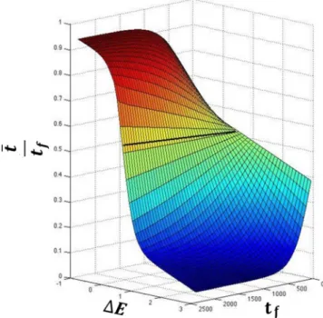
From Fig.1, it can be seen that if either force constant,klor kr, the relative energy differ-ence between the two wells, (DE), or tf are changed, then the minimum action path that the system will take would be different. This means that for different values of DE and tf, and as noted previously,33 there are different minimum action paths between the given equilibrium states, each defined by a differentt. As previously mentioned, sincet uniquely identifies each path, when plotted against different values ofDEandtf, it gives rise to the surface that we call the convergence surface (Fig.2).
This surface represents all the possible minimum action trajectories between a given pair of structures and it is different for different pairs of structures. The bi-sigmoidal functional form of this surface is discussed inAppendix C. This surface also means that multiple, locally minimum action paths are possible for the same pair of structures. Appropriate values of both
DE and tf must therefore be chosen to identify a single minimum action path and transition state that is closest to what is observed in nature.
As mentioned earlier, the force constants are calculated from the Hessian matrix, which is built using a scale constant that is obtained by fitting crystallographic B values to the mean-square
fluctuations of atoms in the structure.2Hence, their accuracy depends strongly on the resolution of the X-ray data. This restriction appears to limit the application of PATH to high resolution crystal structures. Alternately, force constants can, in principle, be determined iteratively by perturbative methods. Parameter estimation can thus require tens of simulations, compromising on the relative speed of PATH simulations. An alternate method to calculate the force constants must be used to elevate the applicability of PATH to that of a general method for studying protein conformational changes.
In the following, we describe these parameters in greater detail, in the context of PATH computations and the convergence surface, and then outline a general strategy for estimating appropriate values of these parameters.
THEORY OF PATH
A significant advantage of the string method31,38 is that it calculates the Minimum Free Energy Path (MFEP) between two equilibrium states. The MFEP must be contrasted with the Minimum Energy Path (MEP) that minimizes the Freidlin-Wentzell action,27 which is the low temperature homolog of the Onsager-Machlup action. Thus, significant parallels emerge between MEP trajectories that minimize the latter action (previously termed “resistance”3) and MFEP that minimize the Onsager-Machlup action. The essential difference between the two approaches is that entropic changes play no role at zero temperature. Pinski and Stuart33 showed that the effects of temperature are of little significance, provided there was no energy difference between initial and final states, but that significant energy differences between states introduced compara-ble changes in the transition states obtained at different temperatures when minimizing the Freidlin-Wentzell action functional. The relevance of free-energy differences between initial and final conformational states emphasizes the value of minimizing the Onsager-Machlup action functional as a useful approximation to the computationally intensive string method. PATH18 implements such an algorithm.
FIG. 2. From Fig.1, it can be seen that the path must depend on bothtfandDE. Sincet, at each value oftf, uniquely identifies a path as a function ofDE, it gives rise to the convergence surface shown in this figure. The surface was fitted to simulations of the catalytic step of TrpRS (R2
PATH simulates the dynamics of a protein molecule by computing the solution to the equation of motion derived from the minimization of the Onsager-Machlup functional, using the Euler-Lagrange equations [Appendix A]. For studying conformational changes between two different equilibrium structures, PATH represents the two structures using a double well potential well (a lin-earized ANM) and uses a separate equation of motion for the dynamics within each potential well.
In the case of a simple diatomic system in one dimension (Fig. 3), the Onsager-Machlup equations of motion are written as
xlð Þ ¼t aþðxaÞ sinhð Þklt sinhðkltÞ
when tt;
(1)
xrð Þ ¼t bþðbxÞ sinh krðttfÞ
sinhðkrðtf tÞÞ !
when tt; (
(2)
wheret is the time taken to reach the transition state,tf is the total time for transition,xis the transition state, aand bare the initial and the final states, respectively, kl andkr are the force constants for the initial and the final states, respectively.
For a smooth transition from one well to the other, the paths have to satisfy boundary con-ditions based on position and velocity. We express these concon-ditions mathematically in the fol-lowing way:
xlðt!tÞ ¼xrðt tfÞ; _
xlðt!tÞ ¼xr_ ðt tfÞ: (3)
Also xlð0Þ ¼a;xrðtfÞ ¼band xðtÞ ¼x, where xl andxr are the trajectories in the left and right well, respectively.
For multiatom 3D system, the interactions between the atoms are more complex, and in the case of a linearized ANM the interaction matrix is a hessian matrix [Appendix B]. Then, the equations of motion can be written as
xlð Þ ¼t V t
t 0
0 sinh k
i lt
sinh kilt
0 B B B @ 1 C C C Aw 2 6 6 6 4 3 7 7 7
5þa; (4)
xrð Þ ¼t W
tf t
tft 0
0
sinh kirðttfÞ
sinh kirðtftÞ
0 B B B B B B @ 1 C C C C C C A / 2 6 6 6 6 6 6 4 3 7 7 7 7 7 7 5
þb; (5)
where w ¼VTðxaÞ;/ ¼WTðxbÞ. V and W are the eigenvectors of the Hessian matrices
of the initial and final wells, and kil andk i
r are their eigenvalues. The eigenvalues replace the
force constants in the trajectory equations because by diagonalizing the Hessian matrix, we
generate 3N normal modes whose individual motion depends on the rate at which the structure changes, which is given by the eigenvalues. The final trajectory is generated by a linear combi-nation of the normal modes.
To solve for the transition state, we apply velocity continuity
V 1 t 0 0 k i lcoshkilt
sinhki lt
0 B @ 1 C A |fflfflfflfflfflfflfflfflfflfflffl{zfflfflfflfflfflfflfflfflfflfflffl} L w 2 6 6 6 6 4 3 7 7 7 7 5 ¼W 1
ttf 0
0 ki
rcosh k i rðttfÞ
sinh ki rðttfÞ
0 B B @ 1 C C A |fflfflfflfflfflfflfflfflfflfflfflfflfflfflfflfflfflfflffl{zfflfflfflfflfflfflfflfflfflfflfflfflfflfflfflfflfflfflffl} R / 2 6 6 6 6 6 4 3 7 7 7 7 7 5 ; (6)
which can be rewritten, to compute the transition state, as
x¼VLV
T
aWRWTb
VLVTWRWT : (7)
Once the transition state is identified, the difference in energy between the two equilibrium states can then be evaluated as
DE¼ðxbÞ
T
PðxbÞ
2
xa
ð ÞTQðxaÞ
2 ; (8)
DEcan also be defined as the energy difference between the transition state energies relative to the two equilibrium states.
In Equations(6)and(7), the unknowns aret andttf, which can also be written astland
tr, such that tlþtr¼tf. As noted earlier, estimating the input tfis crucial for generating a cor-rect transition state using PATH. As the parameters DE andtf are related via the convergence surface (Fig.2), this also means that evaluation oftfis essential for the estimation ofDE.
Simulations of several systems using PATH indicate that the structure of the transition state becomes invariant astfis large. In the case of the 1D diatomic system, we generated the convergence surface and calculated the DE values for different t and tf values. For a constant t
tf of 0.5, we observed that at large values of tf the values of DE are invariant. This also means that the structure of the transition state is a constant. This result implies that the value of tf is immaterial as long as it is large but this assumption gives rise to another problem with PATH parameters. At extremely large values of tf, we observe that the path spends most of its time near the equilibrium structures and uses a fraction of the total time to change the conformation of the protein. Also we observed that the system spent more time in the nar-rower (more energetic) well than in the wider well. This behavior contradicts statistical mechanics. But, at the same time, once the conformational change starts, the system takes less time to climb up the potential well in the narrower well than in the wider well, which is consistent with statistical mechanics.
For protein conformational changes, like domain motions that depend on large frequency rigid-body motions, we describe multiple lines of evidence that no essential information is lost by truncating the initial, invariant portion of the trajectory during which the structure does not change. To resolve this problem, we realized that the system must be given just enough time for the transition state to converge and no more. We therefore truncate the PATH trajectory by beginning only when the system has moved away from aby at least 10% of the total distance between the equilibrium state and the transition state. This is an arbitrary choice; using 1% of the distance fromawould change the resulting transition state almost imperceptibly.
An appropriate value of tf can be calculated for the 1D diatomic system in the following way. Using(1), a general trajectory equation can be written as
x tð Þ ¼aþðxaÞsinhð Þkt
sinhð Þkt ; (9)
whent! 1,(9)becomes
xðtÞ ¼aþ ðxaÞekðttÞ: (10)
As we are interested in the time at which the system has changed by at least 10%,
ekðttÞ¼0:1; (11)
which gives
topt)tt¼2:302
k : (12)
This equation directly computes t for a 1D diatomic system but for multiatom systems in 3D, there are multiple interatomic interactions, and hence multiple force constants associated with the diagonalized Hessian matrix. Hence, we calculated the average force constant for a structure which is the average of the trace of the Hessian
k¼tr Hð Þ
3N ; (13)
whereNis the number of atoms.
The new path algorithm avoids an iterative search
The MinActionPath algorithm18calculates the structure of the transition statexusing the veloc-ity continuveloc-ity equation(6)by assuming a value oft based on the given value oftf. Then, thisxis validated by checking if it satisfies the energy equation(8)for a given value of DE. Ifxdoes not satisfy the energy equation, then a new value oft is assumed and a newx is identified. This pro-cess is repeated until a value oft is found for whichxsatisfies the energy continuity requirement.
In the new algorithm, using (13), topt is directly evaluated from the force constants. This
topt is used to identify the transition state structure directly, without iteration, which speeds up the PATH calculations by an order of magnitude, thereby simplifying, and substantially increas-ing the speed of an already fast method. Usincreas-ing this modified algorithm to calculate topt, we calculated the transition state for three different systems and compared the structures with those generated from other simulation methods.
RESULTS
methods agree closely on the configurations of their transition states. Second, we show that the PATH transition states are close to the saddle points of free-energy surfaces connecting initial and final states generated by replica-exchange Discrete Molecular Dynamics simulations.10,11,34 We show that aromatic side-chain rearrangements create similar potential energy barriers in the transition-state structures identified by PATH for a signaling protein, a contractile protein, and an enzyme.
PATH and ANMPathway trajectories agree most closely with string method trajectories at their transition states
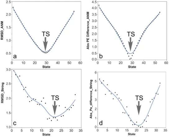
We compared trajectories from the simulations of the converter domain from myosin VI performed using the string method,31 ANMPathway, and PATH. Since the reaction coordinates of the three trajectories are different, it would be difficult to compare them at every instant. We compare in Fig.4the structural similarity and energetic properties of the string transition state as evaluated according to the linearized ANM force field used by PATH. For both comparisons, subset of structures in the string trajectory that was structurally most similar to the PATH tran-sition state (Fig. 4(a)) was the same subset for which the absolute potential energy difference between those calculated with respect to the initial and final states, was closest to zero (Fig. 4(b)). In the context of PATH, the structure whose corresponding potential energy difference is zero is, by definition, the transition state.
We performed a similar analysis with the myosin conformational change trajectory from the ANMPathway method.8 We found that when the PATH transition state is compared with the ANMPathway trajectory, the structures are the closest [root mean squared deviation (RMSD) 0.52 A˚ ] near the transition state of the ANMPathway trajectory [Fig. 4(c)]. Similarly, the same group of structures have the absolute potential energy difference closest to zero [Fig.4(d)].
Discrete molecular dynamics replica exchange simulations verify that transition states identified by path are close to saddle points in the free energy surface connecting initial and final states
The main reason we undertook to study conformational transition state structures was to extend what previously had been established for the structural reaction profile of the B. stearo-thermophilus tryptophanyl-tRNA synthetase (TrpRS; Kapustina et al.21). TrpRS passes through three distinct structural states:
• an Open state that can be stabilized either by stoichiometric amounts of tryptophan or by
sub-stoichiometric amounts of MgATP (adenosine triphosphate)
• a closed, Pre-TS, stabilized by stoichiometric amounts of MgATP and a tryptophan
analog
• a closed, Product state (Pdt), stabilized either by the bound intermediate adenylate product,
tryptophanyl-50AMP, or by stable analogs thereof
As the ligands bind to the Open state, the protein undergoes an induced fit conformational change and goes to the Pre-TS state. At the Pre-TS state, a subsequent catalytic step takes the Pre-TS state to the Pdt state. Both induced-fit and catalysis are slow, relative to the chemical transformation of the substrates; each is therefore associated with a different conformational transition state. Preliminary analysis with the PATH program had given us descriptive accounts of the two transitions.
• Induced-fit proceeds by an early and higher energy barrier that matches the behavior seen by
MD simulations of the TrpRS monomer23
• Catalysis proceeds by a later, lower barrier transition state in which the volume of the
trypto-phan binding pocket assumes a minimum value immediately after the conformational transition state identified by PATH.41
The earlier MD calculations relating to the Induced-fit transition were short, 10 ns lations, and represented what appeared to be a slower conformational change. As MD simu-lations led to a confirmation of the results PATH had given for the Induced-Fit transition,23 we decided to see whether similar, but more detailed simulations might allow a more strin-gent test of results the PATH algorithm had given for the catalytic transition. As the cata-lytic transition represents what is likely a more rapid conformational change with a lower barrier, we carried out replica exchange calculations using DMD,10,11,34 with sufficiently long equilibrations to appropriately sample the free energy surface connecting the Pre-TS and Pdt states.
These calculations produced two notable results:
• The apparent free energy difference between the Pre-TS and Product states depends strongly
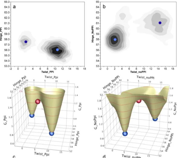
on the presence of the bound product, pyrophosphate (PPi). If the PPi was retained in the bind-ing pocket by a harmonic potential, the equilibrium was far on the side of the Pre-TS state (Fig. 5(a)). On the other hand, if this potential (or constraints) mimicking PPi binding was relaxed or omitted, we observe rapid PPi release and the distribution of states exhibits higher probability towards product state (Fig.5(b)). This behavior is especially interesting in view of the possibility that early release of orthophosphate following actin binding triggers the myosin V powerstroke.32
• Transition states for the transitions with and without the harmonic potential restraining the PPi
output by PATH fall close to the coordinates of the saddle points of the respective energy surfa-ces (Figs.5(c)and5(d)).
Transition states identified by PATH display comparable rate-limiting structures in three different systems
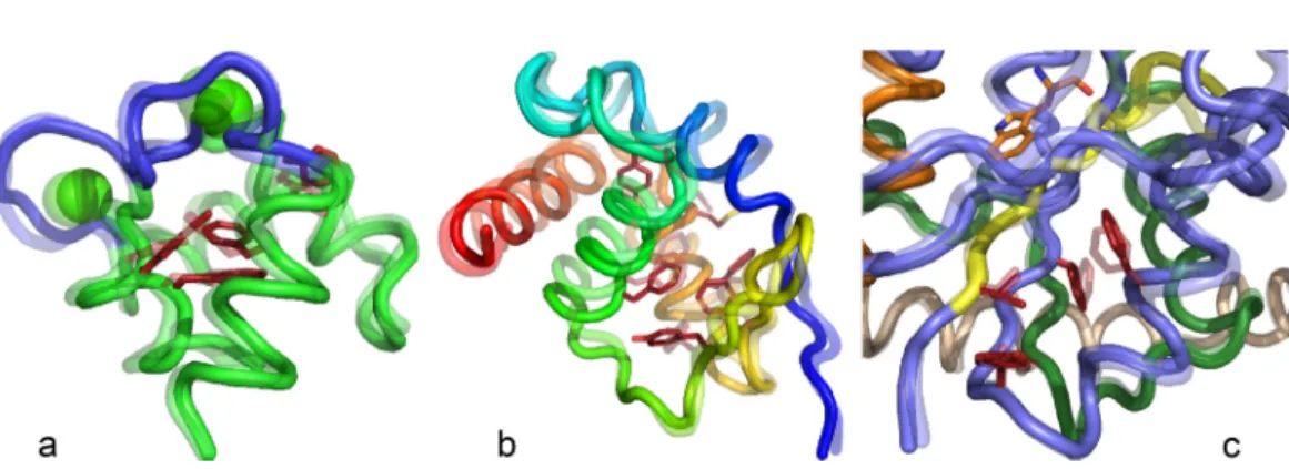
We began these studies to access structural information about the transient conformational tran-sition state(s) that appear to be rate-limiting for TrpRS catalysis.21 In the course of the work, we found it useful also to investigate PATH behaviors of other model systems, including the 1D sys-tem described earlier here. Two well-defined protein conformational transitions–Ca2þrelease by the Ca2þ-binding domain of calmodulin and the converter domain of myosin VI–also proved useful in verifying the generality of aspects described in the Theory of PATH section. These studies reveal a remarkable similarity in all three transition-states (Fig.6). In each case, the rate-limiting conforma-tional change involves re-packing of multiple aromatic side chains4,5,22associated with subtle rear-rangements of the surrounding backbone chains. Such rearrear-rangements are known to occur on a far slower timescale (ls to ms (Ref.35)) than rotamer exchanges of aliphatic side chains in hydropho-bic core regions. Further, the timings of the three transition states (middle, late, early) are consistent with the overall equilibrium constant for the conformational change, via Hammond’s postulate.
CONCLUSIONS
We have reviewed a substantial literature on the methodology of computing trajectories for conformational changes from what is essentially a hybrid between technical and lay per-spectives, consistent with our own interest in the biochemical importance of conformational transition states. In the process, we have de-mystified much previous work in what we hope are useful ways. A remarkable aspect of that literature is that it has yet to describe either the struc-tural details of the cooperative side chain behavior that comprise the barrier or the functional implications of conformational transition states. To contribute usefully to that discussion, we have here tried to address these two aspects of conformational trajectories.
PATH affords a rapid, accurate way to assess the structural features that limit the rate of conformational changes. PATH computations can be performed in a manner that circumvents the problem of defining the four required input parameters. In identifying the mathematical ori-gin of the time-course anomalies and a workable algorithm for choosing appropriate tf values, we have established a basis for more widespread use of the PATH algorithm. One important potential benefit of the broader investigation into details of conformational transition states would be to facilitate the identification of specific residues likely to be involved in allosteric communication, as we have done with TrpRS,21,40,41 thereby enhancing the role of combinato-rial mutagenesis to investigate higher-order coupling in protein functions.
We have provided persuasive evidence that minimization of the Onsager-Machlup action with the PATH algorithm produces a transition state in good agreement with that provided by the String Method and by ANMPathway. The most probable path is generally considered to define a smooth curve through the center of a tube in pathspace.14 Opinions differ, however, over the effective diameter of such a tube, and/or whether multiple tubes might pass through
FIG. 6. Conformational transition state structures for Calmodulin Ca2þ-binding domain (a), Myosin VI converter domain
different transition states.26We show here that three distinct algorithms based on different force fields, using different sets of collective variables to define the pathspace identify quite similar transition state structures. That observation suggests that functionally distinct domain configura-tions in proteins are separated by well-defined structural barriers.
Further, transition states identified by PATH coincide closely with stationary points of free energy surfaces derived using replica-exchange DMD simulations. That evidence validates the use of PATH by a wider group of potential users interested in structural details of the coopera-tive side chain rearrangements26 that limit conformational changes in proteins of interest. Further, our demonstration that residues involved in limiting the TrpRS conformational changes can be implicated in long-range coupling to the active site40,41 suggests that PATH may be useful in identifying candidates for a broad range of combinatorial mutational analyses of enzy-matic Fig.6(c), signaling Fig.6(a), and contractile Fig.6(b)mechanisms.
The observation that quite similar side-chain configurations limit the conformational changes of three quite distinct proteins points to a more general phenomenon in which nature chooses to build multi-state behavior in similar ways. This conclusion has potentially deeper significance because the transition states we have described are more or less independent of whether side chains are included in the simulations. ANMPathway simulations are necessarily performed with onlyCaatoms, and we performed PATH simulations both with all-(heavy)atom and Ca only coordinate files. The resulting transition states are almost indistinguishable (RMSD¼0.25 A˚ for Ca atoms). We cannot account for this coincidental behavior except to note that it suggests a higher-order coupling between side-chain and backbone behavior.7,24 That behavior is, however, reminiscent of our observation that combinatorial point mutation of residues limiting the rate of domain movement during induced-fit in TrpRS show that those residues are coupled to the catalytic activation of the active-site Mg2þion40and to specific rec-ognition of tryptophan41 by essentially the same free energies as those coupling the anticodon-binding and the CP1 insertion domains to catalysis and recognition.25
MATERIALS AND METHODS
Structures
We use three TrpRS structures in our studies. These structures were derived from the crystal structures of the three conformations of TrpRS, namely, Open (1MAW,1MB2), Pre-TS (1MAU) and Pdt (1I6L). We excised the terminal aminoacid (R328) from the structures as it is not observed in most of the crystal structures. We believe that its absence would not affect the con-formational change of the rest of the protein. The ligands in the binding pockets are different for the different states of TrpRS. To make the ligands consistent in all the three structures, we used Tryptophan, AMP, PPi as separate molecules in the binding pocket; the distance between these molecules changes, depending on the state and the chemical species that they represent. We have previously used a similar arrangement23 and this allows approximating the chemical reac-tion without requiring the use of quantum calculareac-tions. The myosin VI structures for the rigor state and the prepowerstroke state were derived from 2BKH and 2V26, respectively. As described in Ref.31, only residues 703–788, which form the converter domain, were used in the simulations. The equilibrium structures for calmodulin were derived from 1CMF and 1FW4.
Path simulations
ANMPathway simulations
The ANMPathway calculations8 were set up on the ANMPathway server. Default input force constants¼0.1 were used for both the energy wells. All the other parameters were set to their default values–Cutoff - 15 A˚ , Energy offset - 0, Step size (on cusp) - 0.8, Step size (slide down) - 0.04 and Target RMSD - 0.1 A˚ .
DMD simulations
Replica Exchange Discrete Molecular Dynamics (REX/DMD) simulations were set up with the Pdt state structure described previously. A harmonic potential was applied between the atoms of the ligands and all the surrounding atoms within 3.5 A˚ to retain the ligands within the binding pocket. In general, replica exchange simulations are used for efficient sampling of the conformational landscape of a given system. However, we were only interested in monitor-ing the transition between the Pdt and Pre-TS state. To facilitate the exploration of this particu-lar transition event as well as to expedite the sampling, we introduced weak harmonic constraints to guide the system progressing from Pdt to Pre-TS state. By comparing the native contacts within the two systems (as obtained from their crystal structures), we extracted the unique contacts that were present in the Pre-TS and not the Pdt state. Those contacts were used as experimental constraints. The DMD force field is currently equipped to work only with Cu2þ or Zn2þ. Since ATP is complexed with Mg2þin in the Pre-TS state, we replaced it with Zn2þ. We believe that this replacement would not affect the conformational change of the protein in a significant way. We simulated parallel replicas at 24 temperatures ranging from 175 K to 405 K for a total duration of 2.5 million steps (125 ns) as described in detail in Ref.42. As the system requires 500 000 steps to equilibrate, all our analyses were performed with the remaining 2 million steps. Snapshots were generated every 1000 steps, hence all our analyses (Fig.5) include 2000 snapshots.
Fitting the free energy surfaces
Each of the 2000 snapshots from the lowest temperature replica exchange DMD simulation was segregated in 225 bins of equal size, based on their Hinge and Twist angles. Based on the distribution of structures within these bins, the free energy surface is computed using the formula
DG¼ kBTln 100 ni
N
;
whereniis the number of structures in the ithbin and N is the total number of structures. Then, these free energy values are fitted to the following equation to generate the free energy surfaces in Fig.5,
DG¼CþAe
ðXTw1Þ2 2SigTw1þ
YH1
ð Þ2 2SigH1þ
J XðTw1ÞðYH1Þ
2 ffiffiffiffiffiffiffiffiffiffiffiffiffiffiffiffiffiffiSigTw12þSigH12
p
þBe
ðXTw2Þ2 2SigTw2þ
YH2
ð Þ2 2SigH2þ
L XðTw2ÞðYH2Þ
2 ffiffiffiffiffiffiffiffiffiffiffiffiffiffiffiffiffiffiSigTw22þSigH22
p
þD Xð TwtÞ þF Xð TwtÞ2þG Yð HtÞ þH Yð HtÞ2;
where X and Y are the Twist and Hinge angles and the constants Tw1, H1, Tw2, and H2 are the twist and hinge, respectively, of the Pdt and Pre-TS structures and Twt and Ht are coordi-nates of the saddle point.
ACKNOWLEDGMENTS
String method trajectory for the myosin converter domain. J. Hermans contributed considerable helpful discussion. C.W.C., Jr. is grateful to J. Roach for help fitting the convergence surface in Fig.2and to M. Delarue for his hospitality at Institut Pasteur and to the Fulbright Foundation for a Research Fellowship during which this work was initiated. This work was supported by NIGMS 40906.
APPENDIX A: EQUATIONS OF MOTION FOR THE MOST PROBABLE PATH
PATH is based on the ANM, in which the interatomic interactions are modeled on vibrating springs. In general, such a system follows Newtonian mechanics and the path that the system takes is the path of least action. In addition to that, PATH considers the dynamics of such a system to be stochastic in nature and models the system to follow the Langevin equation of motion and replaces the classical action with the OM action. In this section, we describe PATH and OM action by com-paring them with the familiar classical spring system.
Classical action
Consider a 1D diatomic system following Newtonian dynamics in a single potential well. The equation of motion can be derived by identifying the path that minimizes action. Since the path is deterministic, the probability,p, of this path is always equal to 1. But to compute this path, it is required to know the kinetic and potential energies of the system.
Potential energy can be calculated from the interaction between the two atoms. As mentioned previously, the two atoms are considered to be connected by a Hookean spring, and the interaction between the atoms is considered to be harmonic in nature. Hence, we write the potential energy as
V xð Þ ¼k 2ðxaÞ
2; (A1)
whereais the equilibrium distance between the two atoms, and xais the displacement from the equilibrium positiona.
Since the kinetic energy of the system isT¼1 2mx_
2, we write the Lagrangian as
L¼TV¼1 2 mx_
2
k xð aÞ2
: (A2)
Using(A2), we write the equation for classical action as
Scl¼ ðt
0
L:dt¼ ðt
0
1 2 mx_
2
k xð aÞ2
dt: (A3)
Equation(A3)computes the action of any given path but we have to find the path of minimum action. Since action is a functional, its extremum is calculated using a variational principle. In Lagrangian mechanics (using the Lagrangian to derive Newton’s equation of motion), this boils down to finding the solution to the Euler-Lagrange equation
@L
@x d dt
@L
@x_ ¼0: (A4)
On applying the boundary conditions,B1andB2, which are, at timet1,x(t1)¼x1andt2,x(t2)¼x2,
the solution to the Euler-Lagrange equation gives the following trajectory equation:
x tð Þ ¼aþ 1 sinðxðt2t1ÞÞ
x1a
ð Þsinðxðt2tÞÞ ðx2aÞsinðxðt1tÞÞ
; (A5)
where x¼ ffiffiffik m
q
is the angular frequency. This is the equation of motion of a spring following
To calculate the action from(A3), we calculate the velocity of the system, which is
_
x tð Þ ¼ 1
sinðxðt2t1ÞÞ
xðx1aÞcosðxðt2tÞÞ þxðx2aÞcosðxðt1tÞÞ
; (A6)
and the total action of this path is
Scl¼ mx
2 sinðxðt2t1ÞÞ
x1a
ð Þ2þðx2aÞ2
h i
cosðxðt2t1ÞÞ 2ðx1aÞðx2aÞ
h i
: (A7)
Protein conformational change is a stochastic process
Unlike the classical spring, dynamics of protein molecules cannot be considered to be deter-ministic but rather a stochastic process, which is modeled by an overdamped Langevin dynamics equation
mcx_¼ dV xð Þ
dx þ
ffiffiffiffiffiffiffiffiffiffiffiffiffiffiffiffi 2mckBT
p
n; (A8)
wherecis the diffusion coefficient, andnis a delta-correlated Gaussian random (zero mean) force. That is
hnðtÞi ¼0; (A9)
hnðtÞnðt0Þi ¼dðtt0Þ: (A10)
In order to understand the Langevin equation, consider the same diatomic 1D system. Unlike the deterministic and periodic equation for a classical spring, if the Langevin equation describes a stochastic process, it can only calculate probabilities of paths that the system might take. Given the current state x1at timet1, the probability of reaching state x2at a small time incrementDt,
assuming microscopic reversibility, is given by
p xð 2attþDtjx1attÞ ¼
e4kBTk ðx1aÞðx2aÞe
kDt mc
2
1þcoth kDt mc ð Þ
ð Þ
1
4pkBT k 1þcoth kDt
mc
1
2
; (A11)
wherekBis the Boltzmann constant, andTis the temperature. This is the solution to the Fokker-Planck equation.
If the total path is a succession of such states, then the joint probability can be calculated as the product of the probabilities of the individual segments. But since we are interested only in the probability of the most probable path, we calculate this by minimizing the exponent in(A11). To do this, Onsager and Machlup29 developed an interesting method to calculate the trajectory by considering Equation(A11)to be of the form
p/e2SOMmkBT: (A12)
By treating the numerator of the exponent to be analogous to classical action, they were able to simplify it into an integral of the form
SOM¼ 1 2c
ðt
0
mcx_þk xð aÞ
ð Þ2dt; (A13)
Since we have a functional whose minimum value has to be calculated, it can be done by solving the Euler-Lagrange equation and on application of the same boundary conditions as in the classical case,B1andB2, we get the following trajectory equation:
x tð Þ ¼aþ 1
sinhðCðt2t1ÞÞ
x1a
ð ÞsinhðCðt2tÞÞ ðx2aÞsinhðCðt1tÞÞ
; (A14)
whereC¼ k
mc. This is the equation of motion of the minimum action path undergoing stochastic
dynamics, modeled by Langevin equation. From(A14), we calculate the velocity as
_
x tð Þ ¼ 1
sinhðCðt2t1ÞÞ
ððCÞðx1aÞcoshðCðt2tÞÞ ðCÞðx2aÞcoshðCðt1tÞÞÞ: (A15)
And by substituting(A14)and(A15)) to(A13), we calculate the action as follows:
SOM¼ mk
2sinhðCðt2t1ÞÞ
½ðx2aÞ2eCðt2t1Þþ ðx1aÞ2eCðt2t1Þ2ðx2aÞðx1aÞ: (A16)
APPENDIX B: CONSTRUCTING THE HESSIAN FOR A LINEARIZED ANM POTENTIAL
PATH uses a linearized ANM potential to represent interatomic interactions where each atom pair is connected to each other in some manner via springs with a single force constant k. According to ANM,1between any two atoms, then, we have the pair potential
U r i;rj¼1
2k rð rÞ
2
; (B1)
whereriis the position of theith atom,rjthe position of thejth atom. We form the distancerby taking the magnitude of r rirj, pointing from thejth atom to the ith one. This distance is compared to the equilibrium length, the magnitude ofr rirj, where the setfrigN
i¼1is a
speci-fied equilibrium configuration defined by the input crystal structure. This potential still yields a nonlinear set of equations of motion, so we will linearize it and obtain our final effective potential for the system following.
Consider a small displacement from the equilibrium configuration:dri anddrj, then we can constructdr dridrj. The potential, for smalldrreads
U¼1 2
s
r2 X
p;q
rprqdrpdrq; (B2)
where the subscriptspandqrepresent thex,y, andzCartesian coordinates of the vectors. We can define the Hessian to be the matrix implicit in the above summation
hij¼: s
r2
ij
r2
x rxry rxrz
ryrx r2y ryrz
rzrx rzrx r2
z
0 B B @
1 C C
A: (B3)
that any error induced by this assumption will be compensated by the estimation oftffrom the av-erage force constantk.
We want to build the full HessianHfrom these three-by-three blocks. If we refer to the three coordinates of theith atom asxiinx(so thatxhasNsuch entries), andHijgives the three-by-three block ofHat rowi, columnj, then the Hessian is constructed by addinghijfrom (B3) toHiiand
Hjjand subtractinghijfromHijandHji.
In the end, we have a symmetric matrixH2R3N3N, and an equilibrium configurationa2
R3N, the effective potential of the system can be written as
U¼1 2ðxaÞ
T
H xð aÞ: (B4)
APPENDIX C: ANALYTICAL DESCRIPTION OF THE CONVERGENCE SURFACE
The convergence surface in Fig.2shows that different minimum action paths are generated for different input values oftfandDE. Not only do we observe thattvaries with different values of these two input parameters but also we understand that the velocity continuity equation (6) gives rise to this surface.
Though the convergence surface is observed for large proteins and for 1D diatomic systems alike, we can write a simplified equation only for the latter. In this section, we will derive an equa-tion for the convergence surface of the diatomic system from the velocity continuity equaequa-tion.
For the diatomic system in 1D, the most probable trajectory is calculated separately for the left side and the right side from(A14)as(1)and(2). From those two equations, we can derive the velocity continuity equation as
krðxbÞcothðkrðttfÞÞ ¼klðxaÞcothðkltÞ: (C1)
To further simplify this equation, we have to know the structure of the transition state (x), which, in a 1D diatomic system, can be computed by rearranging Equation(8)to
1
2klðxaÞ
2
þDE¼1
2krðxbÞ
2
: (C2)
If the initial structure isa¼(a1,a2) and the final structure isb¼(b1,b2), then we can calculate the
structure of the transition statex¼ ðx1;x2Þby writing the energy continuity equation as
1 2ðxaÞ
kl kl
kl kl
xa
ð ÞTþDE¼1
2ðxbÞ
kr kr
kr kr
xb
ð ÞT: (C3)
The two matrices in Equation(C3)are the Hessian matrices of the initial and final states, as outlined inAppendix B.
We can rewrite Equation(C3)as
kl
2 x1a1 x2a2
1 1
1 1
x1a1
x2a2
þDE
¼kr
2 x1b1 x2b2
1 1
1 1
x1b1
x2b2
:
On simplification, the above equation becomes
kl
2½ðx1x2Þ ða1a2Þ
2þ
DE¼kr
2 ðx1x2Þ ðb1b2Þ
2
: (C4)
kl
2ðXAÞ
2
þDE¼kr
2ðXBÞ
2
: (C5)
Solving forX
X ¼
klAkrB
ð Þ ðABÞ
ffiffiffiffiffiffiffiffiffiffiffiffiffiffiffiffiffiffiffiffiffiffiffiffiffiffiffiffiffiffiffiffiffiffiffiffiffiffiffi
krklþ2DE krð klÞ
BA
ð Þ2
s
klkr
ð Þ : (C6)
For a diatomic system centered on the origin,x1þx2¼0, giving, together withX, the transition
state,x.
This transition state structure can be substituted into the velocity continuity equation (C1), and simplified to
sinhkrtfðkrþklÞt
sinhkrtfðkrklÞt
¼ krþkl krkl
2krkl
ZDEðkrklÞ
; (C7)
whereZ¼ ffiffiffiffiffiffiffiffiffiffiffiffiffiffiffiffiffiffiffiffiffiffiffiffiffiffiffiffiffiffiffikrklþ2DEBðkrklÞ A ð Þ2 q
, andklandkr correspond to eigenvalues of the respective Hessian matrices.
In any spring system in one dimension, the overall motion is comprised ofN independent modes, each with its own force constant. In the case of the diatomic system, there is one transla-tional mode, whose force constant is zero and one vibratransla-tional mode. Since each mode behaves in-dependently from the other, the spring constant associated with each mode is calculated from the eigenvalues of the respective Hessian matrices. Sincetfis known, we can calculatetof the 1D dia-tomic system, numerically. Thus, the entire landscape of path trajectories shown in Fig.2can be computed from Equation(C7). This equation also describes the bi-sigmoidal behavior of the con-vergence surface. For constant values oftf,thas a sigmoidal relationship toDE. Similarly at con-stantDE,t has a sigmoidal relationship totf, though the shape of the curve in Fig.2is that of a rectangular hyperbola. This behavior rises from the use of positive values oftf, as negative values oftfare meaningless.
1A. R. Atilgan, S. R. Durell, R. L. Jernigan, M. C. Demirel, O. Keskin, and I. Bahar, “Anisotropy of fluctuation dynamics
of proteins with an elastic network model,”Biophys. J.80(1), 505–515 (2001).
2I. Bahar, A. R. Atilgan, and B. Erman, “Direct evaluation of thermal fluctuations in proteins using a single-parameter
har-monic potential,”Folding Des.2(3), 173–181 (1997).
3M. Berkowitz, J. Morgan, and J. McCammon, “Diffusion controlled reactions: A variational formula for the optimum
reaction coordinate,”J. Chem. Phys.79, 5563–5565 (1983).
4S. K. Burley and G. A. Petsko, “Aromatic-aromatic interaction: A mechanism of protein structure stabilization,”Science
229, 23–28 (1985).
5S. K. Burley and G. A. Petsko, “Amino-aromatic interactions in proteins,”FEBS Lett.203(2), 139–143 (1986). 6
C. W. J. Carter, “Tryptophanyl-tRNA synthetases,” in The Aminoacyl-tRNA Synthetases, edited by M. Ibba, C. Francklyn, and S. Cusack (Landes Biosciences/Eurekah.com, Georgetown, TX, 2005), pp. 99–110.
7
C. Clementi, H. Nymeyer, and J. N. Onuchic, “Topological and energetic factors: What determines the structural details of the transition state ensemble and en-route intermediates for protein folding? an investigation for small globular proteins,”J. Mol. Biol.298(5), 937–953 (2000).
8A. Das, M. Gur, M. H. Cheng, S. Jo, I. Bahar, and B. Roux, “Exploring the conformational transitions of biomolecular
systems using a simple two-state anisotropic network model,”PLoS Comput. Biol.10(4), e1003521 (2014).
9F. Ding and N. V. Dokholyan, “Emergence of protein fold families through rational design,”PLoS Comput. Biol.
2(7), 0725–0733 (2006).
10F. Ding, D. Tsao, H. Nie, and N. V. Dokholyan, “Ab initio folding of proteins with all-atom discrete molecular
dynami-cs,”Structure16(7), 1010–1018 (2008).
11N. V. Dokholyan, S. V. Buldyrev, H. E. Stanley, and E. I. Shakhnovich, “Discrete molecular dynamics studies of the
fold-ing of a protein-like model,”Folding Des.3(6), 577–587 (1998).
12N. V. Dokholyan, S. V. Buldyrev, H. E. Stanley, and E. I. Shakhnovich, “Identifying the protein folding nucleus using
molecular dynamics,”J. Mol. Biol.296, 1183–1188 (2000).
13N. V. Dokholyan, L. Li, F. Ding, and E. I. Shakhnovich, “Topological determinants of protein folding,”Proc. Natl Acad.
Sci. U.S.A.99(13), 8637–8641 (2002).
14D. Durr and A. Bach, “The Onsager-Machlup function as Lagrangian for the most probable path of a diffusion process,”
Commun. Math. Phys.60, 153–170 (1978).
15E. Weinan, W. Ren, and E. Vanden-Eijnden, “String method for the study of rare events,”Phys. Rev. B
16
P. Faccioli, “Characterization of protein folding by dominant reaction pathways,” J. Phys. Chem. B 112(44), 13756–13764 (2008).
17
P. Faccioli, M. Sega, F. Pederiva, and H. Orland, “Dominant pathways in protein folding,”Phys. Rev. Lett.97(10), 108101 (2006).
18
J. Franklin, P. Koehl, S. Doniach, and M. Delarue, “MinActionPath: Maximum likelihood trajectory for large-scale struc-tural transitions in a coarse-grained locally harmonic energy landscape,”Nucleic Acids Res.35, W477–W482 (2007).
19
A. Ghosh, R. Elber, and H. A. Scheraga, “An atomically detailed study of the folding pathways of protein A with the sto-chastic difference equation,”Proc. Natl. Acad. Sci. U.S.A.99(16), 10394–10398 (2002).
20M. Kapustina and C. W. Carter, “Computational studies of tryptophanyl-tRNA synthetase: Activation of ATP by
induced-fit,”J. Mol. Biol.362(5), 1159–1180 (2006).
21M. Kapustina, V. Weinreb, L. Li, B. Kuhlman, and C. W. Carter, “A conformational transition state accompanies
trypto-phan activation byB. stearothermophilustryptophanyl-tRNA synthetase,”Structure15(10), 1272–1284 (2007).
22E. Lanzarotti, R. R. Biekofsky, D. A. Estrin, M. A. Marti, and A. G. Turjanski, “Aromatic aromatic interactions in
pro-teins: Beyond the dimer,”J. Chem. Inf. Model.51, 1623–1633 (2011).
23P. Laowanapiban, M. Kapustina, C. Vonrhein, M. Delarue, P. Koehl, and C. W. Carter, “Independent saturation of three
TrpRS subsites generates a partially assembled state similar to those observed in molecular simulations,”Proc. Natl. Acad. Sci. U.S.A.106(6), 1790–1795 (2009).
24Y. Levy, S. S. Cho, J. N. Onuchic, and P. G. Wolynes, “A survey of flexible protein binding mechanisms and their
transi-tion states using native topology based energy landscapes,”J. Mol. Biol.346, 1121–1145 (2005).
25L. Li, C. Francklyn, and C. W. Carter, “Aminoacylating urzymes challenge the RNA world hypothesis,”J. Biol. Chem.
288(37), 26856–26863 (2013).
26P. Maragakis and M. Karplus, “Large amplitude conformational change in proteins explored with a plastic network
model: Adenylate kinase,”J. Mol. Biol.352(4), 807–822 (2005).
27
L. Maragliano, A. Fischer, E. Vanden-Eijnden, and G. Ciccotti, “String method in collective variables: Minimum free energy paths and isocommittor surfaces,”J. Chem. Phys.125(2), 24106 (2006).
28
L. K. Nicholson and K. P. Lu, “Prolylcis-transisomerization as a molecular timer in Crk signaling,”Mol. Cell25(4), 483–485 (2007).
29
L. Onsager and S. Machlup, “Fluctuations and irreversible processes,”Phys. Rev.91(6), 1505–1512 (1953).
30J. N. Onuchic and P. G. Wolynes, “Theory of protein folding,”Curr. Opin. Struct. Biol.14, 70–75 (2004). 31
V. Ovchinnikov, M. Karplus, and E. Vanden-Eijnden, “Free energy of conformational transition paths in biomolecules: The string method and its application to myosin VI,”J. Chem. Phys.134(8), 085103 (2011).
32
V. Ovchinnikov, B. L. Trout, and M. Karplus, “Mechanical coupling in myosin V: A simulation study,”J. Mol. Biol. 395(4), 815–833 (2010).
33
F. J. Pinski and A. M. Stuart, “Transition paths in molecules at finite temperature,”J. Chem. Phys.132(18), 184104 (2010).
34D. Shirvanyants, F. Ding, D. Tsao, S. Ramachandran, and N. V. Dokholyan, “Discrete molecular dynamics: An efficient
and versatile simulation method for fine protein characterization,”J. Phys. Chem. B116(29), 8375–8382 (2012).
35J. J. Skalicky, J. L. Mills, S. Sharma, and T. Szyperski, “Aromatic ring-flipping in supercooled water: Implications for
NMR-based structural biology of proteins,”J. Am. Chem. Soc.123, 388–397 (2001).
36N. D. Socci, J. N. Onuchic, and P. G. Wolynes, “Protein folding mechanisms and the multidimensional folding funnel,”
Proteins: Struct., Funct., Genet.32, 136–158 (1998).
37Y. Sugita and Y. Okamoto, “Replica-exchange molecular dynamics method for protein folding,”Chem. Phys. Lett.
314(1–2), 141–151 (1999).
38
E. Vanden-Eijnden and M. Venturoli, “Revisiting the finite temperature string method for the calculation of reaction tubes and free energies,”J. Chem. Phys.130(19), 194103 (2009).
39
E. D. Watt, H. Shimada, E. L. Kovrigin, and J. P. Loria, “The mechanism of rate-limiting motions in enzyme function,”
Proc. Natl. Acad. Sci. U.S.A.104(29), 11981–11986 (2007).
40
V. Weinreb, L. Li, and C. W. Carter, “A master switch couples Mg2þ-assisted catalysis to domain motion inB. stearo-thermophilustryptophanyl-tRNA synthetase,”Structure20(1), 128–138 (2012).
41
V. Weinreb, L. Li, S. N. Chandrasekaran, P. Koehl, M. Delarue, and C. W. Carter, “Enhanced amino acid selection in fully evolved tryptophanyl-tRNA synthetase, relative to its urzyme, requires domain motion sensed by the D1 switch, a remote dynamic packing motif,”J. Biol. Chem.289(7), 4367–4376 (2014).
42
B. Williams II, M. Convertino, J. Das, and N. V. Dokholyan, “ApoE4-specific misfolded intermediate identified by mo-lecular dynamics simulations,”PLOS Comput. Biol.11(10), e1004359 (2015).
43